VLSI Architecture Design of Fractional Motion Estimation for H.264/AVC

DOI 10.1007/s11265-008-0213-7

VLSI Architecture Design of Fractional Motion

Estimation for H.264/AVC

Yi-Hau Chen· Tung-Chien Chen · Shao-Yi Chien ·

Yu-Wen Huang· Liang-Gee Chen

Received: 7 March 2006 / Revised: 18 March 2008 / Accepted: 12 April 2008 / Published online: 4 June 2008 © 2008 Springer Science + Business Media, LLC. Manufactured in The United States

Abstract The H.264/AVC Fractional Motion

Estima-tion (FME) with rate-distorEstima-tion constrained mode decision can improve the rate-distortion efficiency by 2–6 dB in peak signal-to-noise ratio. However, it comes with considerable computation complexity. Accelera-tion by dedicated hardware is a must for real-time applications. The main difficulty for FME hardware im-plementation is parallel processing under the constraint of the sequential flow and data dependency. We ana-lyze seven inter-correlative loops extracted from FME procedure and provide decomposing methodologies to obtain efficient projection in hardware implementa-tion. Two techniques, 4×4 block decomposition and efficiently vertical scheduling, are proposed to reuse data among the variable block size and to improve the hardware utilization. Besides, advanced architec-tures are designed to efficiently integrate the 6-taps 2D

Y.-H. Chen (

_B

DSP/IC Design Lab., Graduate Institute of Electronics Engineering and Department of Electrical Engineering, National Taiwan University, 1, Sec. 4, Roosevelt Rd., Taipei 10617, Taiwan e-mail: ttchen@video.ee.ntu.edu.tw T.-C. Chen e-mail: djchen@video.ee.ntu.edu.tw S.-Y. Chien e-mail: sychien@video.ee.ntu.edu.tw Y.-W. Huang e-mail: yuwen@video.ee.ntu.edu.tw L.-G. Chen e-mail: lgchen@video.ee.ntu.edu.tw

finite impulse response, residue generation, and 4×4 Hadamard transform into a fully pipelined architec-ture. This design is finally implemented and integrated into an H.264/AVC single chip encoder that supports realtime encoding of 720×480 30fps video with four reference frames at 81 MHz operation frequency with 405 K logic gates (41.9% area of the encoder).

Keywords H.264/AVC· Motion estimation ·

VLSI architecture· Video coding

1 Introduction

Digital video compression techniques play an impor-tant role that enables efficient transmission and storage of multimedia content in bandwidth and storage space limited environment. The newly established video cod-ing standard, H.264/AVC [1–3], which is developed by the Joint Video Team significantly outperforms previous standards in both compression performance and subjective view. It can saves 25%–45% and 50%– 70% of bitrates when compared with MPEG-4 [4] and MPEG-2 [5], respectively. While highly interactive and recreational multimedia applications appear much faster than expected, H.264/AVC starts to play an im-portant role in this area due to its higher compression ratio and better video quality. .

The improvement in compression performance mainly comes from the new functionalities, but these new functionalities, especially inter prediction, cause significantly large computation complexity. In H.264/ AVC, inter prediction, which is also called Motion Estimation (ME), can be divided into two parts — Integer ME (IME) and Fractional ME (FME). The

Figure 1 The rate-distortion

curves under three predicted resolution : integer pixel, half pixel, and quarter pixel. Four sequences with different characteristics are used for the experiment. Foreman stands for general sequence with media motions. Mobile and Optis have complex textures. Soccer has large motions. The parameters for above sequences are 30frames/s, 1 reference frames and low complexity mode decision. For QCIF, D1 and HD 720p sequences, the search range is±16-pel, ±32-pel and ±64-pel, respectively. a Foreman (QCIF). b Mobile (QCIF).

c Soccer (D1). d Optis (HD 720p). 28 30 32 34 36 38 40 42 44 28 30 32 34 36 38 40 42 44 28 30 32 34 36 38 40 42 44 30 280 530 780 1030 200 1200 2200 3200 4200 5200 200 6200 12200 18200 24200 (Kbps) (Kbps) (Kbps) (dB) (dB) (dB) Quarter Pixel Half Pixel Integer Pixel 28 30 32 34 36 38 40 42 44 200 700 1200 1700 2200 (Kbps) (dB) Quarter Pixel Half Pixel Integer Pixel (a) (b) (c) (d) Integer Precision Half Precision Quarter Precision Integer Precision Half Precision Quarter Precision

IME searches for the initial prediction in coarse reso-lution. Then, FME refines this result to the best match in fine resolution. Several fast algorithms and hardware architectures are proposed for H.264/AVC IME [6–9], but not for FME. According to our analysis, the FME occupies 45% [10] of the run-time in H.264/AVC in-ter prediction and upgrades rate-distortion efficiency by 2–6 dB in peak signal-to-noise ratio as shown in Fig. 1. However, the FMEs in previous standards contribute only a very small computation complexity. Besides, the Variable Block Sizes (VBS), Multiple Reference Frames (MRF) [11], Lagrangian mode deci-sion [12,13], and many other encoding issues are not involved. Therefore, the traditional FME architec-tures [14, 15] cannot efficiently support H.264/AVC. Obviously, the new and advanced architecture of FME unlike previous standards is urgently demanded in the H.264/AVC compression system.

The main difficulty for the hardware implementation of FME is parallel processing under the constraint of the sequential mode decision flow and data depen-dency. The Lagrangian mode decision is done after the costs of all blocks and sub-blocks in every ref-erence frame with quarter-pel precision are derived. According to our analysis, the FME flow contains seven inter-correlative loops including interpolation, residue

generation, and Hadamard transform. Several tech-niques including 4×4 block decomposition and effi-cient vertical scheduling are proposed to effieffi-ciently parallelize several loops in the hardware. The corre-sponding architecture is designed with features of high utilization, fully pipelined, and reusability.

The rest of this paper is organized as follows. The background, including the related functionality and mode decision flow, is introduced in Section 2. In Section 3, seven loops sketching the FME procedure are analyzed. Then, the efficient architecture includ-ing Motion Compensation function is proposed in Section 4. The implementation and integration results will be shown in Section 5. Finally, conclusions are drawn in Section6. t t-1 t-2 t-3 t-4 Figure 2 MRF ME.

16x16 16x8 8x16 8x8

8x8 8x4 4x8 4x4

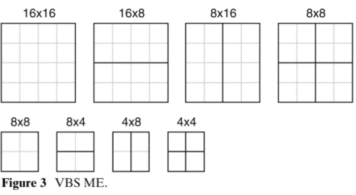
Figure 3 VBS ME.

2 Overview of H.264/AVC FME

In this section, technical overview of H.264/AVC FME will be introduced. Then, the whole procedure includ-ing mode decision flow will be described and the com-putation complexity through profiling will be shown. 2.1 Functionality Overview

In H.264/AVC, FME supports quarter-pixel accuracy with VBS and MRF. For MRF-ME shown in Fig.2, more than one prior reconstructed frames can be used as reference frames. This tool is effective for the un-covered backgrounds, repetitive motions, and highly textured areas [16]. For VBS-ME, the block size in H.264/AVC ranges from 16×16 to 4×4 luminance sam-ples. As shown in Fig.3, the luminance component of each Macroblock (MB) can be selected from four kinds of partitions: 16×16, 16×8, 8×16, and 8×8. For the partition 8×8, each 8×8 block can be further split into four kinds of sub-partitions: 8×8, 8×4, 4×8, and 4×4. This tree-structured partition leads to a large number of possible combinations within each MB. In general,

i1 i2 i3 h1 i4 i5 i6 h2 h3 h4 h5 h6 h0 h1 = round((i1-5xi2+20xi3+20xi4-5xi5+i6+16)/32) h0 = round((h1-5xh2+20xh3+20xh4-5xh5+h6+16)/32) i1 h1 i2 h3 i3 h5 i4 h2 h4 q1 q4 q2 q3 i# : Integer pixel f# : half pixel q# : quarter pixel q1 = (i1+h1+1) / 2 q2 = (i1+h2+1) / 2 q4 = (h1+h3+1) / 2 q3 = (h1+h2+1) / 2 (a) (b)

Figure 4 Interpolation scheme for luminance component: a 6-tap

FIR filter for half pixel interpolation b Bilinear filter for quarter pixel interpolation.

large blocks are appropriate for homogeneous areas, and small partitions are beneficial for textured area and objects of variant motions. The accuracy of motion compensation is in quarter-pel resolution for H.264/ AVC, which can provide significantly better compres-sion performance, especially for pictures with complex texture. Six-tap finite impulse response (FIR) filter is applied for half pixel generation as shown in Fig. 4a, and bilinear filter for quarter pixel generation as shown in Fig. 4b. Quarter-pel resolution Motion Vectors (MVs) in the luminance component will require eighth-pel resolution in each chrominance component.

The mode decision algorithm is left as an open is-sue in H.264/AVC. In the reference software [17], the Lagrangian cost function is adopted. Given the quan-tization parameter QP and the Lagrange parameter

λMODE (a QP dependent variable), the Lagrangian mode decision for a MB MBkproceeds by minimizing

JMODE(MBk, Ik|QP, λMODE)

= Distortion(MBk, Ik|QP) + λMODE · Rate(MBk, Ik|QP)

where the MB mode Ik denotes all possible coding modes and MVs. The best MB mode is selected by considering both the distortion and rate parts. Due to the huge computation complexity and sequential issues in the high complexity mode of H.264/AVC, it is less suitable for real-time applications. In this paper, we focus on low complexity mode decision. The distor-tion is evaluated by the Sum of Absolute Transformed Differences (SATD) between the predictors and origi-nal pixels. The rate is estimated by the number of bits required to code the header information and the MVs. Figure 5shows the best partition for a picture with different quantization parameters. With larger QP, the mode decision tends to choose the larger block or the modes with less overhead in the MB header. In contrast, when the QP is small, it tends to choose the smaller block for more accurate prediction.

2.2 FME Procedure in Reference Software

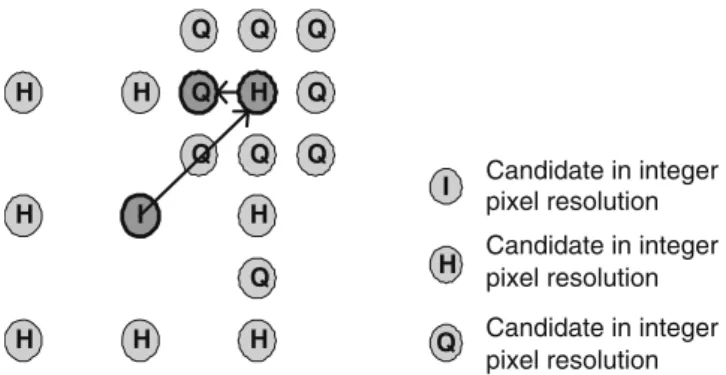
Figures6and7show the refinement flow and procedure of FME in the H.264/AVC reference software [17], respectively. To find the sub-pixel MV refinement of each block, a two-step refinement is adopted for every block. In Fig. 6, the half-pixel MV refinements are performed around the best integer search positions, I, from IME results. The search range of half-pixel MV refinements are±1/2 pixel along both horizontal and vertical directions. The quarter-pixel ME, as well, is

Figure 5 Best partition

for a picture with different quantization parameters (black block: inter block, gray

block: intra block). a QP = 0. b QP = 25. c QP = 51.

(a) (b) (c)

then performed around the best half search position with±1/4 pixel search range. Each refinement has nine candidates, including the refinement center and its eight neighborhood, for the best match.

In Fig.7, the best MB mode is selected from five can-didates: Inter8×8, Inter16×16, Inter16×8, Inter8×16, and skip mode, denoted as S1–S5. In S1 procedure, each 8×8 block should find its best sub-MB mode from four choices: Sub4×4, Sub4×8, Sub8×4, and Sub8×8, denoted as a–d. Thus, nine sub-blocks are processed for each 8×8 block, and a total of 41 blocks and sub-blocks are involved per reference frame. The inter mode deci-sion is done after all costs are computed in quarter-pel precision in all reference frames. Please note that the sub-blocks in each 8×8 block should be within the same reference frame.

Based on reference software, the derivation of matching cost of each candidate can be shown as Fig. 8. The reference pixels are interpolated to pro-duce fractional pixels for each search candidate. Afterward, residues are generated by subtracting the corresponding fractional pixels from current pixels. Then, the absolute values of the 4×4-based Hadamard transformed residues are accumulated as distortion cost called SATD. The final matching cost is calculated by adding the SATD with the MV cost. Taking MV cost into consideration improves the compression

perfor-I H H H H H H H H Q Q Q Q Q Q Q Q Q Q H I Candidate in integer pixel resolution Candidate in integer pixel resolution Candidate in integer pixel resolution

Figure 6 FME refinement flow for each block and sub-block.

mance for VBSME, but brings many data dependencies among blocks because of the MV predictor defined in H.264/AVC standard. The cost can be correctly derived only after prediction modes of the neighboring blocks are determined.

2.3 Profiling

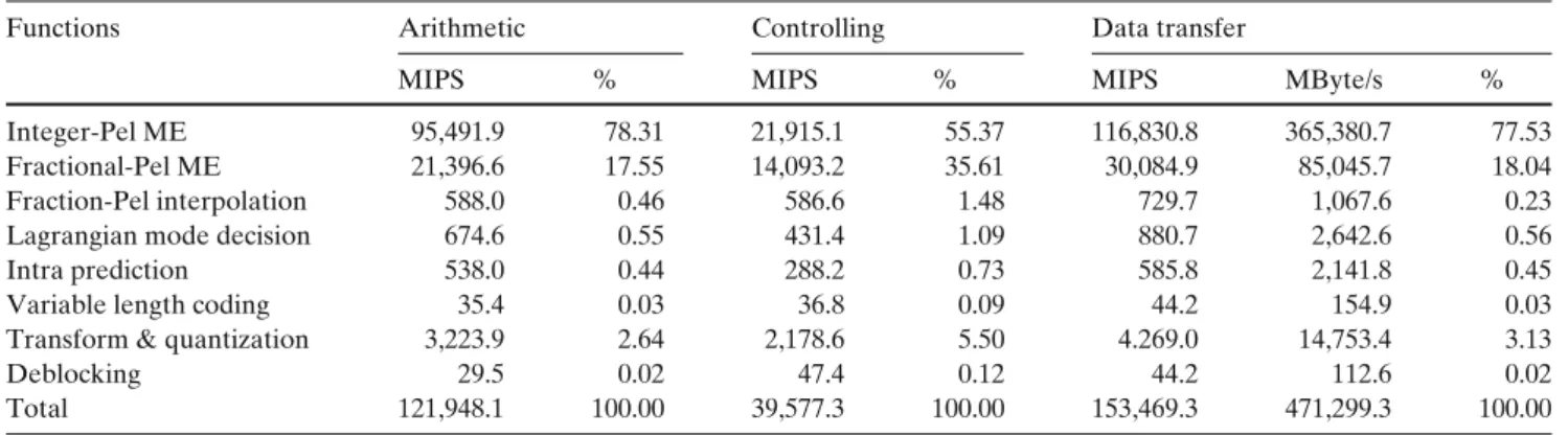
We use iprof, a software analyzer at the instruction level, to generate the profiling of an H.264/AVC en-coder at a processor-based platform (SunBlade 2000 workstation, 1.015 GHz Ultra Sparc II CPU, 8 GB RAM, Solaris 8). The instructions are divided into three categories - computing (arithmetic and logic operations), controlling (jump and branch), and mem-ory access (data transfer such as load and store). Table 1 shows the result of instruction profiling. Ac-cording to the profiling result, the encoding complexity of H.264/AVC is about ten times more complex than MPEG-4 [18]. The high complexity comes from inter prediction with MRF and VBS. For FME, the com-plexity is proportional to the product of the number of block types and the number of reference frames. The required huge computation is far beyond the capability of today’s General Purpose Processors, not to mention

a. Sub4x4 : Refine four sub-blk4x4 b. Sub4x8 : Refine two sub-blk4x8 c. Sub8x4 : Refine two sub-blk8x4 d. Sub8x8 : Refine sub-blk8x8 e. Mode decision for blk8x8 Up-left 8x8 Procedures Up-right 8x8 Procedures Down-left 8x8 Procedures Down-right 8x8 Procedures S2. Inter16x16 : Refine blk16x16

S1. Inter8x8 : Refine four blk8x8

S3. I nter16x8 : Refine two blk16x8 S4. Inter8x16 : Refine two blk 8x16 S5. Check Skip Mode

Sets of IMV

S6. Final Mode Decision for a MB

MV s and ref-frames of best predicted MB

Figure 7 FME procedure of Lagrangian inter mode decision in

Hadamard Transform Interpolation

+

+

Figure 8 The matching cost flowchart of each candidate.

about the higher specification such as HDTV applica-tions. The hardware accelerator of FME is definitely required.

3 FME Procedure Decomposition

According to the analysis in the previous sections, the FME in H.264 greatly enhances the rate distortion efficiency, but also contributes to considerable compu-tation complexity. Obviously, the FME of H.264/AVC must be accelerated by the dedicated hardware. The main challenge here is to achieve parallel processing under the constraints of sequential FME procedure. The hardware utilization and control regularity must be well considered during the realization of the VBS func-tionality. Since the data throughput of 6-taps 2D FIR filter, residue generation and 4×4 Hadamard transform are quite different, it is hard to integrate these func-tional blocks into a fully pipelined design. In this sec-tion, we will simplify the complex encoding procedure into several encoding loops, and two decomposing

tech-niques are proposed to parallelize the algorithm while maintaining high hardware utilization and achieving vertical data reuse.

3.1 Analysis of Encoding Loops

Based on the operating flow in H.264/AVC reference software, we can decompose the entire FME procedure in Figs. 6, 7 and Fig. 8 into seven iteration loops as shown in Fig. 9a. The first two loops are reference frames and the 41 blocks with seven different sizes, respectively. The third loop is the refinement procedure of half-pixel precision and then quarter-pixel precision. The next two loops are the 3×3 candidates of each refinement process. The last two loops are iterations of pixels for each candidate, and range from 16×16 to 4×4. The main tasks inside the most inner loops are the fractional pixel interpolation, residue generation, and Hadamard transform. Note the three main tasks have different input/output throughput rates.

For the realtime constraint, some of the loops must be unrolled and efficiently mapped into the parallel hardware. The costs of a certain block in different ref-erence frames can be processed independently. There-fore, the first loop can be easily unrolled for parallel processing by duplicating multiple basic FME Process-ing Units (PUs) for MRF issue. For the second loop, since 41 MVs of variable block types may point to different position, the required memory bitwidth of Search Window will be too large if the reference pixels of VBS are read in parallel. Besides, the definition of MV predictors also force the 41 MVs to be processed sequentially. The third loop should still be processed sequentially because quarter refinement is based on result of half refinement.

In original FME procedure, the costs of 3×3 search candidates are processed independently. However, the

Table 1 Instruction profile of an H.264/AVC baseline profile encoder.

Functions Arithmetic Controlling Data transfer

MIPS % MIPS % MIPS MByte/s %

Integer-Pel ME 95,491.9 78.31 21,915.1 55.37 116,830.8 365,380.7 77.53

Fractional-Pel ME 21,396.6 17.55 14,093.2 35.61 30,084.9 85,045.7 18.04

Fraction-Pel interpolation 588.0 0.46 586.6 1.48 729.7 1,067.6 0.23

Lagrangian mode decision 674.6 0.55 431.4 1.09 880.7 2,642.6 0.56

Intra prediction 538.0 0.44 288.2 0.73 585.8 2,141.8 0.45

Variable length coding 35.4 0.03 36.8 0.09 44.2 154.9 0.03

Transform & quantization 3,223.9 2.64 2,178.6 5.50 4.269.0 14,753.4 3.13

Deblocking 29.5 0.02 47.4 0.12 44.2 112.6 0.02

Total 121,948.1 100.00 39,577.3 100.00 153,469.3 471,299.3 100.00

PS : The encoding parameters are CIF, 30frames/s, 5 reference frames,±16-pel search range, QP=20, and low complexity mode decision. MIPS stands for million instructions per second.

Parallelized as hardware engine Mapped to FSM Loop1 (Reference Frame)

Loop6 (9 candidates for each refinement) Loop7 (4 Pixels in a row)

{ Sub-Pixel Interpolation Residue Generation Hadamard Transform } Loop2 (41 MVs of Different Block Sizes)

Loop3 (Half- or Quarter-Precision) Loop5 (Height of a Block or Subblock) Loop4 (Horizontal rows of 4-pixels ) Loop1 (Reference Frame)

Loop2 (41 MVs of Different Block Sizes) Loop4 (3 Vertical Search Positions)

Loop5 (3 Horizontal Search Positions) Loop3 (Half- or Quarter-Precision)

Loop6 (Height of a Block or Subblock) Loop7 (Width of a Block or Subblock) { Sub-Pixel Interpolation Residue Generation Hadamard Transform } Left for adaptability (a) (b)

Figure 9 a Original FME procedure. b Rearranged FME procedure with 4×-block decomposition and vertical data reuse.

interpolated pixels for the nine search candidates are highly overlapped. As shown in Fig. 10, the search candidates, which are numbered as 1, 3, 7, 9, have more than nine overlapped interpolated pixels in one 4× 4 block. It is beneficial to parallel processing these nine search candidates because the interpolated pixels can be greatly reused for adjacent candidates to save re-dundant computations and processing cycles. For the last two loops, the iteration numbers depend on block size. Here we propose two techniques to decompose the iteration loops and improve hardware utilization in the following two subsections.

3.2 4×4-Block Decomposition

In H.264/AVC, the 4×4 block is the smallest element for all blocks, and the SATD is also based on 4×4 trans-form blocks. Every block and subblock in a MB can be

Figure 10 The example of overlapped interpolated pixels

between different search candidates in a 4× 4 block. The squares are the integer pixels, and the circles represent interpolated half pixels. Each search candidate requires 4× 4 pixel data. Nine search candidates which are listed from 1 to 9 are processed to compare cost. The numbers listed in each circle are the search candidate numbers to which the corresponding interpolated pixel belongs.

decomposed into several 4×4-elements with the same MV. Therefore, we can concentrate on designing a 4 ×4-element PU and then apply the folding technique to reuse the 4×4-element PU for all block sizes. Figure11

takes one 4×8 block as an example. One 4×8 block is decomposed into the upper and bottom 4×4 element blocks. These 4×4 element blocks are processed in the sequential order, and the corresponding SATDs are accumulated for the final costs.

According to the loop analysis, we will arrange nine 4×4-element PUs to process the 3×3 candidates simul-taneously. In this way, the interpolated half pixels can be reused by these 4×4-element PUs. The redundant computation of interpolation can be saved, and the memory bandwidth to access reference integer pixels can be reduced. Because of the limited output bit-width of internal memory and whole encoder consideration [19], search window memory is assumed to support 1-D random access in this design. Thus, only the adjacent integer pixels in the same horizontal row can be ac-cessed in one cycle. Therefore, each 4×4-element PU is designed to simultaneously process four horizontally adjacent pixels for residue generation and Hadamard transform. In this way, most horizontally adjacent inte-ger pixels can be reused by horizontal filters, and the bandwidth requirement of search window memory can be further decreased.

Figure 12 Main concepts of FME design: a 4×4-block

decompo-sition; b vertical data reuse.

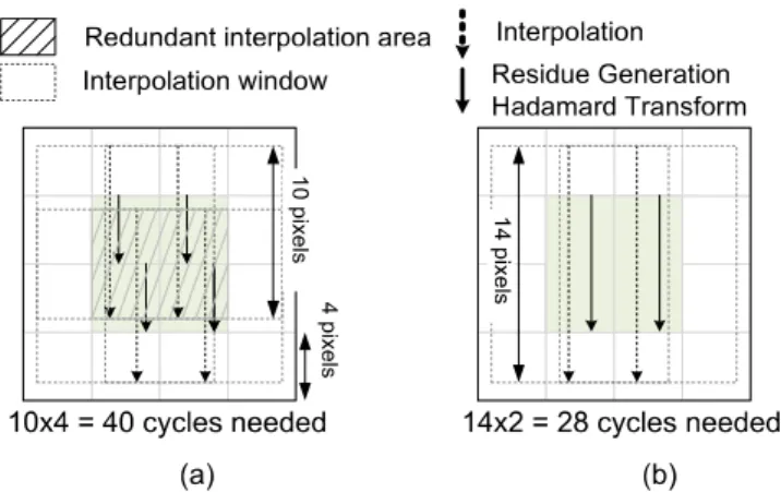
For a single 4×4 block, in order to interpolate the re-quired pixels for nine candidates with 6-taps FIR filter, 10×10 integer pixels are required. As shown in Fig.11, the dotted square denotes the required integer pixels for interpolation, which is called interpolation window. The dotted arrow denotes the interpolation operation while the solid arrow represents the residue generation and Hadamard transform. The interpolation procedure dominates the operation time. Since a row of horizontal integer pixels can be accessed in one cycle, ten cycles are required to process one 4×4-element. It requires 20 cycles to process a 4×8 sub-block.

3.3 Efficient Scheduling for Vertical Data Reuse After the 4×4-block decomposition, redundant inter-polation operations appear in the overlapped area of adjacent interpolation windows. As shown in Fig.12a, one 8×8 block will be divided into four 4×4-elements with the corresponding interpolation windows. The solid square with slash denotes the half pixels gen-erated in the processes of both the upper and bot-tom 4×4-elements. Please note that the operation time

is dominated by the interpolation. If the overlapped interpolation results can be reused, both the hardware utilization and the throughput will be increased.

As shown in Fig.12b, the interpolation windows of vertically adjacent 4×4-elements are integrated. Four-teen cycles used to access 10×14 integer pixels are required for each 4×8-element, and totally 28 (14×2) cycles are required for one 8×8 block. After efficient scheduling for vertical data reuse, 30% of the cycles are saved, and the PU’s utilization is improved from 40% to 57% for 8×8 block. In fact, the improvement varies with the height of each block, and is summarized in Table 2. The average utilization of 4×4-PUs and interpolation circuit are 54% and 100%, respectively.

Figure9b shows the rearranged loops. In summary, there will be nine PUs to process the nine candidates in parallel. In one candidate, four horizontally adjacent pixels are handled simultaneously. The upper region of the rearranged loops will be mapped to a finite state machine as a control unit, and the lower gray part will be accelerated by the dedicated computing unit with a total of 36 times of parallelism in terms of residue generation. Please note that the reference frame loop is left to be adaptively adjusted according to the specifi-cation. The FME tasks in different reference frames can be either parallelized by multiplying the computational cores or scheduled by FSM.

4 Hardware Architecture of Parallel FME Unit

In this section, we will describe the proposed architec-ture for FME module with the procedure characterized by regular flow and efficient hardware utilization, which we mentioned in previous section. Figure 13 shows the block diagram of parallel FME unit comprised of nine 4×4-block PUs per reference frame to thor-oughly parallelize the rate-constrained mode decision.

Table 2 Hardware utilization of different block sizes.

Block 4x4 block decomposition With vertical data reuse size

Blocks / Cycles / PU Interpolation Blocks / Cycles / PU Interpolation MB block utilization (%) utilization (%) MB block utilization (%) utilization (%)

16×16 16 10×1 40 100 1 22×4 73 100 16×8 16 10×1 40 100 2 14×4 57 100 8×16 16 10×1 40 100 2 22×2 73 100 8×8 16 10×1 40 100 4 14×2 57 100 8×4 16 10×1 40 100 8 10×2 40 100 4×8 16 10×1 40 100 8 14×1 57 100 4×4 16 10×1 40 100 16 10×1 40 100 Total 1120 40 100 832 54 100

4x4 Block PU0 4x4 Block PU1 4x4 Block PU8 . . . ACC0 . . . Best Mode Buffer MV Cost Generator Mode Cost Generator ACC1 ACC8 Lagrangian mode decision

Best Mode Info. MC Mux Intepolation Reference Pixels (10 pixel) Original Pixels (4 pixel) MC Predictors (4 pixels) Best Mode Info.

Figure 13 Block diagram of the FME engine.

All side information and the SATD are considered in the matching criterion. The loops of 3×3 search points are unrolled, so there are nine 4×4-block PUs to process nine candidates around the refinement cen-ter. Each 4×4-block PU is responsible for the residue generation and Hadamard transform of each candi-date. The interpolation engine generates the half or quarter reference pixels based on current refinement step. These interpolated pixels are shared by all 4 ×4-block PUs to achieve data reuse and local bandwidth reduction. ACC accumulates the SATD value of each decomposed 4×4 element block. The final candidate cost is generated after the corresponding MV cost is added. The “Lagrangian mode-decision” engine is re-sponsible for the sequential procedures of the 1st–5th loops in Fig.9b. The information of best match block is latched in the “BEST Mode Buffer”. In order to achieve resource sharing (reuse interpolation engine) and system bandwidth reduction (reuse search window memory), motion compensation is allocated in the same MB pipeline stage [20]. The predicted pixels for mo-tion compensamo-tion are generated by the interpolamo-tion engine and then selected by “MC Mux” according to the information in the “BEST Mode Buffer”. The com-pensated MB will be buffered and transmitted to the next stage for the rest coding procedure.

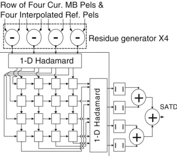
The architecture of each 4×4 PU is shown in Fig.14. Four subtractors generate four residues in each cycle and transmit them to the 2-D Hadamard transform

unit. The 2-D Hadamard transform unit [21] contains two 1-D transform units and one transposed register array. For each 4×4 block, the first 1-D transform unit filters the residues row by row and the second 1-D transform unit processes the transformed residues column by column. The data path of the transposed registers can be configured as rightward shift or down-ward shift. The two configurations interchange with each other every four cycles. First, the rows of 1-D transformed residues of the first 4×4 block are writ-ten into transpose registers horizontally. After four cycles, the columns of 1-D transformed residues are read vertically for the second 1-D Hadamard transform. Meanwhile, the rows of 1-D transformed residues of the second 4×4 block are written into transposed registers vertically. In this way, the Hadamard transform unit is fully pipelined with residue generators. The latency of the 2-D transform is four cycles, and there is no bubble cycle between vertically adjacent 4×4 blocks.

Figure 15a shows the parallel architecture of 2-D interpolation engine. The operations of 2-D FIR fil-ter are decomposed into two 1-D FIR filfil-ters with the interpolation shifting buffer array. A row of ten hor-izontally adjacent integer pixels are input to generate five horizontal interpolated half pixels simultaneously. These five half pixels and six neighboring integer pixels are latched and shifted downward in the “V-IP Unit” as shown in Fig. 15b. After the latency of six cycles, the eleven vertical filters generate 11 vertical half pix-els by filtering the six pixpix-els within the corresponding “V-IP Units”. The dotted rectangle in the bottom of

1-D Hadamard 1 - D H a d a m a r d SATD Residue generator X4 | | | | | | | |

-

-

-

-+

+

+

2-D Hadamard Transform Unit Row of Four Cur. MB Pels & Four Interpolated Ref. Pels

Figure 15 Block diagram of

interpolation engine (a, b).

HFIR HFIR HFIR HFIR HFIR

V - I P U n i t 0 1 V - I P U n i t 0 2 V - I P U n i t 0 3 V - I P U n i t 0 4 V - I P U n i t 0 5 V - I P U n i t 0 6 V - I P U n i t 0 7 V - I P U n i t 0 8 V - I P U n i t 0 9 V - I P U n i t 1 0 V - I P U n i t 1 1 I V V H V V I V V H V V I V V H V V I V V H V V I V V H V V I V V Quarter Pixel Bilinear Interpolation Engine Mux

Half Or Quarter 4x4-PUs

Integer Pixel Input Shift Register HFIRHorizontal FIR VFIRVertical FIR

I _{Integer Pixel} H _{Horizontally Filtered Half Pixel} V _{Vertically Filtered Half Pixel}

V F

I R

V-IP Unit

(a) (b)

Fig.15a represents the reference pixels for half-pixel refinement in one cycle. For quarter-pixel refinement, another bilinear filtering engine with input from the dotted rectangle is enabled to generate quarter pixels. For larger blocks, a folding technique is applied to iteratively utilize the interpolation circuits and PUs. An efficient vertical scheduling in Section3.3is proposed to reuse interpolated pixels in the “V-IP Units”, and 26% of cycles can be saved according to Table2.

5 Implementation Results and Discussion of Reusability

5.1 Implementation Results

The proposed architecture of FME unit in Fig.13 is implemented by UMC 0.18μ 1P6M technology. This architecture can support complete FME procedure de-scribed in Section2.2, and provide the highest compres-sion performance. The motion compensation engine is included to share hardware resource and save system

Table 3 Gate count profile of the FME unit.

Functional block Gate counts Percentage (%) Interpolation unit 23872 30.08

MVCost generator 6477 8.16

4×4-PU x 9 (w. ACC) 34839 43.89 Mode decision engine 2174 2.74

Central control 1538 1.94

InOut buffer 10472 13.19

Total 79372 100.00

bandwidth. The gate count profile is listed in Table3. The interpolation engine and 4×4 block PUs contribute 74% gate count of the whole FME unit, while the Hadamard transform occupies 85% gate count in the 4×4 block PUs. This FME unit has 36 times of parallel-ism per reference frame in terms of residue generation. The proposed FME engine can support SDTV 720× 48030 fps with all MB modes for one reference frame under 77 MHz and this is the first hardware solution for H.264/AVC FME [22]. Table4also shows the compar-ison between the proposed architecture and the newest one. The improved one can further support the higher specifications via higher horizontal parallelism.

5.2 Reusability for Fast Algorithm

The proposed FME engine is based on H.264 reference software to provide full functionality. However, some

Table 4 Comparison between the proposed architecture and the

newest one. Proposed [22] [23] ICASSP-04 ISCAS-06 Technology UMC 0.18 um TSMC 0.18 um Clock freq. 100 MHz 285 MHz Gate counts 79372 188456 Parallelism 4 16 Frame size 720×576 HD1080p Frame rate 30fps 30fps Max. performance 52k MB/s 250k MB/s unit : NAND2 gate count

31 33 35 37 32 34 36 38 60 110 160 210 260 (Kbps) 300 800 1300 1300(Kbps) (dB) (dB) Full Functionalities Hvbi noSATD noVBS MDinIME (a) (b) Full Functionalities Hvbi noSATD noVBS

Figure 16 Analysis of the rate-distortion efficiencies among

dif-ferent functionalities of FME. HVBi: Use bilinear filter instead of 6-tap FIR in FME; noSATD: Use SAD instead of SATD as distortion cost; noVBS: Use only 16× 16 and 8 × 8 block sizes; MDinIME: Mode decision is done in IME phase instead of FME

phase. The parameters for above sequences are 30frames/s, 1 reference frames and low complexity mode decision. The search range is±16-pel and ±32-pel for QCIF and D1 format, respec-tively. a Foreman (QCIF). b Soccer (D1).

trade-offs between hardware cost and compression per-formance can be made by modifying the related encod-ing algorithms. Three methods are taken as examples here. First, the hardware of complex 2-D 6-tap FIR filter can be replaced by simpler bilinear interpolation scheme. It can save 11 vertical FIR and most inter-polation buffer, and reduce about 15% hardware cost. Second, we can use sum-of-absolute-difference (SAD) instead of SATD to estimate the bit-rate influenced by DCT. Thus, the Hadamard transform can be removed and about 40% hardware cost can be saved. Third, since the FME unit is decomposed into 4× 4 block size and controlled by FSM as shown in Fig.9, we can decide how many MB modes are skipped in FME operating procedure to save power consumption and processing cycles without changing the proposed architecture. For example, we can perform FME on 16× 16 and 8 × 8 modes like MPEG-4 or on only the best MB mode from IME. Figure16demonstrates the corresponding rate-distortion performances of above three cases and full functionality mode. Because adopting bilinear fil-ter or SAD results in apparent quality degradation,

it is better to cooperate the proposed FME unit with FME fast algorithm of early-termination mechanism while maintaining coding performances in our newest work [24].

5.3 Reusability for Different Specifications

According to the analysis in Session 3.1, the FME procedures in different reference frames can be either parallelized by duplicating the FME units or scheduled by FSM with one FME unit. Therefore, our FME unit can be reused for different specifications. Table5lists some possible specifications with the corresponding solutions. The processing cycles of each case can be calculated by summing the required cycles of supported block sizes, skip mode, and motion compensation. Take case (a) as example, each refinement cycles of 16×16, 16×8, 8×16 and 8×8 modes are 88×1, 56×2, 44×2, and 28×4, respectively (please referred to Table 2). Because of half/quarter refinements, the number of cycles is then multiplied by two. The cycles required by the skip mode in P-frame is the same as one 16×16

Table 5 Reusability of the proposed FME unit among some possible applications.

Specification Functionality # FME units Cycles/MB Frequency

(a) HDTV(1280× 720 30fps) MRF(3), VBS(16× 16–8 × 8) 3 1000 108 MHz

(b) SDTV(720× 480 30fps) MRF(4), VBS(all) 4 1912 77.4 MHz

(c) CIF(352× 288 30fps) MRF(4), VBS(all) 2 3576 42.5 MHz

(d) QCIF(176× 144 30fps) MRF(5), VBS(all) 1 8568 25.4 MHz

MV Cost Gen.

RefMV Buffer

Interpolation

Luma Ref. Pels SRAMs (Shared with IME) Router

Cur. Luma MB Pels (from IME)

Best Inter Mode Information Buffer Inter Mode Decision Results

(to IP) Cur. Luma MB SRAM FME Controller Encoding Parameters (from Main Control and IME)

Mode Cost Gen. MC Luma MB SRAM MC Luma MB Pels (to IP) 4x4-Block PU #8 Ref. Cost Gen. 9x4 MV Costs

4 Ref. Costs 9x4 Candidate Costs 4x4-Block PU #0 4x4-Block PU #3 4x4-Block PU #1 4x4-Block PU #4 4x4-Block PU #2 4x4-Block PU #5 4x4-Block PU #7 4x4-Block PU #6

Rate-Distortion Optimized Mode Decision

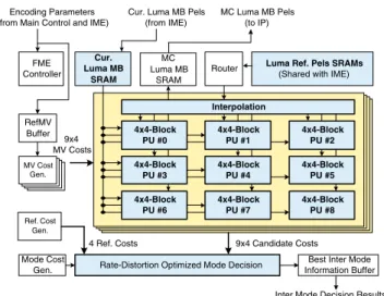
Figure 17 Block diagram of the FME pipeline stage for a single

chip H.264 encoder.

block refinement, while that of motion compensation is the same as one 8×8 block refinement in the worst case. Summing up these components is 1000 cycles. In case (a), three FME units are connected in parallel and each of which is responsible for the task of one reference frame. On the contrary, case (d) represents that a single FME unit processes the tasks of different reference frames sequentially. Thus, more computing cycles are required for one MB, and higher operating frequency is induced compared to case (e). But the hardware cost of case (d) is only one-fifth of case (e).

The proposed architecture has been successfully in-tegrated into a single chip H.264 encoder [19]. This en-coder can real-time process 720×480 30fps video with four MRFs at 81 MHz operation frequency as the case (b) in Table5. Four-MB pipelined scheme is adopted to separate whole encoding procedure into several tasks with their corresponding accelerators [20]. The block diagram of FME pipeline stage is shown in Fig. 17. 41×4 pairs of integer MVs are input from IME pipeline stage, and then the FME refinement procedures are enabled. Four FME units are responsible for four ref-erence frames. The mode decision is finished after all block sizes including skip mode are processed. Then the motion compensation is performed. The search window SRAMs of luminance reference pixels are embedded and shared with IME pipeline stage to reduce the sys-tem bandwidth. The FME results, including the best predicted mode, the corresponding MV’s, and motion compensated pixels, are stored in the buffers and then transmitted to the next stage for the reconstruction and entropy coding procedure. The total gate count of FME stage is 405K gates and occupies 41.91% area of the whole encoder.

6 Conclusion

This paper presents a VLSI architecture design for FME of H.264/AVC. According to our analysis, FME can significantly increase the compression performance with considerable computation complexity. However, acceleration by parallel hardware is a tough job because of the sequential Lagrangian mode decision flow. We analyze the processing loops and provide decomposing methodologies to obtain the optimized projection in hardware implementation. The 4×4 decomposition is proposed for hardware regularity and reusability for VBS, while efficiently vertical scheduling are applied to reuse data and to increase hardware utilization. The corresponding fully pipelined architecture is designed as the first FME hardware solution and implemented in UMC 0.18μ 1P6M technology. Four such FME units can support all FME functionalities of baseline profile Level 3 at 81 MHz operation frequency.

References

1. Joint Video Team (2003). Draft ITU-T recommendation and

final draft international standard of joint video specification,

ITU-T Recommendation H.264 and ISO/IEC 14496-10 AVC (May).

2. Wiegand, T., Sullivan, G. J., Bjøntegaard, G., & Luthra, A. (2003). Overview of the H.264/AVC video coding standard.

IEEE Transactions on Circuits and Systems for Video Tech-nology (CSVT), 13(7), 560–576 (July).

3. Ostermann, J., Bormans, J., List, P., Marpe, D., Narroschke, M., Pereira, F., et al. (2004). Video coding with H.264/AVC: Tools, performance, and complexity. IEEE Magazine on

Circuits and Systems Magazine, 4, 7–28.

4. ISO (1999). Information technology - coding of audio-visual

objects - Part 2: Visual. ISO/IEC 14496-2.

5. ISO (1996). Information technology - generic coding of

moving pictures and associated audio information: Video.

ISO/IEC 13818-2 and ITU-T Rec. H.262.

6. Choi, W.-I., Jeon, B., & Jeong, J. (2003). Fast motion esti-mation with modified diamond search for variable motion block sizes. In Proceedings of IEEE international conference

on image processing (ICIP’03), (pp. 371–374).

7. Huang, Y.-W., Wang, T.-C., Hsieh, B.-Y., & Chen, L.-G. (2003). Hardware architecture design for variable block size motion estimation in MPEG-4 AVC/JVT/ITU-T H.264. In

Proceedings of IEEE international symposium on circuits and systems (ISCAS’03), (pp. 796–799).

8. Lee, J.-H., & Lee, N.-S. (2004). Variable block size motion estimation algorithm and its hardware architecture for H.264. In Proceedings of IEEE international symposium on circuits

and systems (ISCAS’04) (pp. 740–743).

9. Yap, S. Y., & McCanny, J. V. (2004). A VLSI architecture for variable block size video motion estimation. IEEE

Transac-tions on Circuits and Systems II (CASII), 51, 384–389.

10. Chen, T.-C., Fang, H.-C., Lian, C.-J., Tsai, C.-H., Huang, Y.-W., Chen, T.-W., et al. (2006). Algorithm analysis and architecture design for HDTV applications. IEEE Circuits

11. Wiegand, T., Zhang, X., & Girod, B. (1999). Long-term mem-ory motion-compensated prediction. IEEE Transactions on

Circuits and Systems for Video Technology (CSVT), 9, 70–84

(February).

12. Sullivan, G. J., & Wiegand, T. (1998). Rate-distortion op-timization for video compression. IEEE Signal Processing

Magazine, 15(6), 74–90 (November).

13. Wiegand, T., Schwarz, H., Joch, A., Kossentini, F., & Sullivan, G. J. (2003). Rate-constrained coder control and comparison of video coding standards. IEEE Transactions on

Circuits and Systems for Video Technology (CSVT), 13(7),

688–703 (July).

14. Chao, W.-M., Chen, T.-C., Chang, Y.-C., Hsu, C.-W., & Chen, L.-G. (2003). Computationally controllable integer, half, and quarter-pel motion estimator for MPEG-4 advanced simple profile. In Proceedings of 2003 international symposium on

circuits and systems (ISCAS’03) (pp. II788–II791).

15. Miyama, M., Miyakoshi, J., Kuroda, Y., Imamura, K., Hashimoto, H., & Yoshimoto, M. (2004). A sub-mW MPEG-4 motion estimation processor core for mobile video applica-tion. IEEE Journal of Solid-State Circuits, 39, 1562–1570. 16. Su, Y., & Sun, M.-T. (2004). Fast multiple reference frame

motion estimation for H.264. In Proceedings of IEEE

inter-national conference on multimedia and expo (ICME’04).

17. Joint Video Team Reference Software JM8.5 (2004).http:// bs.hhi.de/∼suehring/tml/download/(September).

18. Chang, H.-C., Chen, L.-G., Hsu, M.-Y., & Chang, Y.-C. (2000). Performance analysis and architecture evaluation of MPEG-4 video codec system. In Proceedings of IEEE

international symposium on circuits and systems (ISCAS’00), 2, 449–452 (May).

19. Huang, Y.-W., Chen, T.-C., Tsai, C.-H., Chen, C.-Y., Chen, T.-W., Chen, C.-S., et al. (2005). A 1.3TOPS H.264/AVC Single-Chip Encoder for HDTV Applications. In

Proceed-ings of IEEE international solid-state circuits conference (ISSCC’05) (pp. 128–130).

20. Chen, T.-C., Huang, Y.-W., & Chen, L.-G. (2004). Analysis and design of macroblock pipelining for H.264/AVC VLSI architecture. In Proceedings of 2004 international symposium

on circuits and systems (ISCAS’04) (pp. II273–II276).

21. Wang, T.-C., Huang, Y.-W. Fang, H.-C., & Chen, L.-G. (2003). Parallel 4x4 2D transform and inverse transform architecture for MPEG-4 AVC/H.264. In Proceedings of

IEEE international symposium on circuits and systems (ISCAS’03) (pp. 800–803).

22. Chen, T.-C., Huang, Y.-W., & Chen, L.-G. (2004). Fully uti-lized and reusable architecture for fractional motion esti-mation of H.264/AVC. In Proceedings of IEEE ICASSP (pp. V–9–V–12) (May).

23. Yang, C., Goto, S., & Ikenaga, T. (2006). High performance VLSI architecture of fractional motion estimation in H.264 for HDTV. In Proc. IEEE ISCAS (pp. 2605–2608).

24. Chen, T.-C., Chen, Y.-H., Tsai, C.-Y., & Chen, L.-G. (2006). Low power and power aware fractional motion estimation of H.264/AVC for mobile applications. In Proceedings of IEEE

international symposium on circuits and systems (ISCAS’06).

Yi-Hau Chen was born in Taipei, Taiwan, R.O.C., in 1981. He

received the B.S.E.E degree from the Department of Electri-cal Engineering, National Taiwan University, Taipei, Taiwan, R.O.C., in 2003. Now he is working toward the Ph.D. degree in the Graduate Institute of Electronics Engineering, National Taiwan University. His major research interests include the algorithm and related VLSI architectures of global/local motion estimation, H.264/AVC, scalable video coding.

Tung-Chien Chen was born in Taipei, Taiwan, R.O.C., in

1979. He received the B.S. degree in electrical engineering and the M.S. degree in electronic engineering from National Taiwan University, Taipei, Taiwan, R.O.C., in 2002 and 2004, respectively, where he is working toward the Ph.D. degree in electronics engineering. His major research interests include motion estimation, algorithm and architecture design of MPEG-4 and H.26MPEG-4/AVC video coding, and low power video coding architectures.

Shao-Yi Chien received the B.S. and Ph.D. degrees from the Department of Electrical Engineering, National Taiwan University (NTU), Taipei, in 1999 and 2003, respectively. During 2003 to 2004, he was a research staff in Quanta Research Insti-tute, Tao Yuan Shien, Taiwan. In 2004, he joined the Graduate Institute of Electronics Engineering and Department of Elec-trical Engineering, National Taiwan University, as an Assistant Professor. His research interests include video segmentation al-gorithm, intelligent video coding technology, image processing, computer graphics, and associated VLSI architectures.

Yu-Wen Huang was born in Kaohsiung, Taiwan, in 1978. He

received the B.S. degree in electrical engineering and Ph. D. degree in the Graduate Institute of Electronics Engineering from National Taiwan University (NTU), Taipei, in 2000 and 2004, respectively. He joined MediaTek, Inc., Hsinchu, Taiwan, in 2004, where he develops integrated circuits related to video cod-ing systems. His research interests include video segmentation, moving object detection and tracking, intelligent video coding technology, motion estimation, face detection and recognition, H.264/AVC video coding, and associated VLSI architectures.

Liang-Gee Chen was born in Yun-Lin, Taiwan, in 1956. He

received the BS, MS, and Ph.D degrees in Electrical Engineering from National Cheng Kung University, in 1979, 1981, and 1986, respectively.

He was an Instructor (1981-1986), and an Associate Professor (1986-1988) in the the Department of Electrical Engineering, National Cheng Kung University. In the military service during 1987 and 1988, he was an Associate Professor in the Institute of Resource Management, Defense Management College. From 1988, he joined the Department of Electrical Engineering, National Taiwan University. During 1993 to 1994 he was Visiting Consultant of DSP Research Department, AT&T Bell Lab, Murray Hill. At 1997, he was the visiting scholar of the De-partment of Electrical Engineering, University, of Washington, Seattle. Currently, he is Professor of National Taiwan University. From 2004, he is also the Executive Vice President and the General Director of Electronics Research and Service Organi-zation (ERSO) in the Industrial Technology Research Institute (ITRI). His current research interests are DSP architecture design, video processor design, and video coding system.

Dr. Chen is a Fellow of IEEE. He is also a member of the honor society Phi Tan Phi. He was the general chairman of the 7th VLSI Design CAD Symposium. He is also the general chair-man of the 1999 IEEE Workshop on Signal Processing Systems: Design and Implementation. He serves as Associate Editor of IEEE Trans. on Circuits and Systems for Video Technology from June 1996 until now and the Associate Editor of IEEE Trans. on VLSI Systems from January 1999 until now. He was the Associate Editor of the Journal of Circuits, Systems, and Signal Processing from 1999 until now. He served as the Guest Editor of The Journal of VLSI Signal Processing Systems for Signal, Image, and Video Technology, November 2001. He is also the Associate Editor of the IEEE Trans. on Circuits and Systems II: Analog and Digital Signal Processing. From 2002, he is also the Associate Editor of Proceedings of the IEEE.

Dr. Chen received the Best Paper Award from ROC Com-puter Society in 1990 and 1994. From 1991 to 1999, he received Long-Term (Acer) Paper Awards annually. In 1992, he received the Best Paper Award of the 1992 Asia-Pacific Conference on Circuits and Systems in VLSI design track. In 1993, he received the Annual Paper Award of Chinese Engineer Society. In 1996, he received the Out-standing Research Award from NSC, and the Dragon Excellence Award for Acer. He is elected as the IEEE Circuits and Systems Distinguished Lecturer from 2001-2002.