What can be seen in a noisy optical flow field projected by a moving planar patch in 3D space?

(1)

Pergamon

PII: S0031-3203(96)00174-4

WHAT CAN BE SEEN IN A NOISY OPTICAL FLOW FIELD

PROJECTED BY A MOVING PLANAR PATCH IN 3D SPACE?

SOO-CHANG PEI* and LIN-GWO LIOU

Department of Electrical Engineering, National Taiwan University, Taipei, Taiwan, R.O.C.

(Received 13 July 1995; in revised form 15 May 1996; received for publication 24 October 19961

Abstract--In this paper, we would like to propose a brand new interpretation to the so-called "structure-from- motion" (SFM) problem. The optical flow field projected by a moving rigid planar patch in 3D space is our main consideration. Instead of just obtaining an explicit 3D motion/pose solution like the old approaches did before, we focus our attention on analyzing its error sensitivity, uncertainty, and ambiguity from another point of view. Our new method can handle the above error analysis easily. As known well before, the optical flow field projected by a 3D moving planar patch can be completely expressed by eight coefficients (two for second-order, four for first-order, and two for zeroth-order). Based on these flow coefficients easily determined by a linear regression method or other similar approaches, the error sensitivity of 3D estimates can be analyzed quantitatively and qualitatively in a coarse-to-fine way. The concepts of camera fixation and singular value decomposition (SVD) play important roles in our analysis. There are three goals for our experiments: (1) To prove the correctness of the algorithms (simulated image). (2) To show the tendency of error sensitivity when the 3D poses of the target planar patch are varied in a controlled manner (simulated image). (3) To show that our analysis is workable in the real-world application (real-world image). © 1997 Pattern Recognition Society. Published by Elsevier Science Ltd.

Optical flow field Camera fixation

Perspective projection

Impacting time Affine transform

1. INTRODUCTION

The structure-from-motion (SFM) problem has received considerable attention lately. Its purpose is to recover the 3D motion/structure of a moving object from the change of its projected images. Many methods using image points, lines, contours, optical flow, or normal flow have been developed. In this paper, the optical flow field projected by a moving rigid planar patch (MRPP) in 3D space is our main consideration. The optical flow field used here is defined as the instantaneous positional changes of 2D image points, the same as the definition of a so-called "motion flow field." Although there are several slight differences between the traditional definition of an optical flow field and that of a motion flow field, we do not want to emphasize these differences here and confuse readers.

There has been much research ~1 22~ in estimating the motion/pose of an MRPP in 3D space. For example, using the scaled orthographic projection, there were several area-based (or contour-based) methods: Kanata- ni,<81 Mukundanf9.~l~ YoungflO~ and Pei ~12'131 approxi- mated the change of projected image shapes by a linear (affine) transform. Under the condition that the MRPP is positioned relatively far enough from the camera, the smaller higher-order change of projected image shapes is completely ignored in their analysis.

However, there were other approaches °-71 which adopted the perspective projection (pin-hole camera)

* Author to whom correspondence should be addressed.

as their main image model. In 1985, Waxman

et al. ~1'21 developed the so-called velocity functional method to parameterize the flow field projected by a 3D surface. They concluded that the true optical flow field projected by an MRPP can be completely expressed by eight parameters (two for second-order, four for first- order, and two for zeroth-order). Kanatani ~71 directly used the above flow coefficients to solve 3D motion/ pose of the planar patch. His analysis was described in terms of complex algebra. Of course there were other methods using different image measurements. For example, Kanatani ¢3t used line and surface integrals; Tsai and Huang ~a-61 used four co-planar point features and solved an SVD problem. The most important conclusion made by them is: there are usually two ambiguous solutions (by at least four point correspondences) when solving the 3D motion/pose of an unknown MRPR

In fact, ambiguous solutions always happen no matter what kinds of image measurements are used. Some

researchers<IS 221 are especially interested in the multiple

interpretations of an image flow field projected by an MRPP. They also have a similar conclusion: two planar surfaces undergoing different motions may give rise to the same image motion.

However, most of the above researchers ~ ~-221 focused their attention on the complete determination of 3D parameters, while ignoring the analysis of error sensitivity and uncertainty. As known well from experience, the measurement accuracy of the higher-order flow coefficients is seldom reliable enough for an accurate 3D estimate due to the finite image resolution and noise- 1401

(2)

1402 S.-C. PEI and L.-G. LIOU

sensitive flow measurement. Old approaches just told us the 3D estimates will be poor when the noise is high. But how poor they are? Can it be described quantitatively? How do the 3D poses of an MRPP affect the accuracy of 3D estimates? Does there exist any singular case when solving the unknowns? What can be seen in a (noisy) optical flow field projected by an MRPP? These ques- tions were rarely answered before!

Therefore, in this paper, a new algorithm is proposed to analyze this sensitivity problem from another point of view. Our main concern is to make a quantitative and qualitative analysis of the error sensitivity, not to develop a more robust or simpler algorithm than the old ones.

The concepts of camera fixation (23-2s) and singular value decomposition (SVD) play important roles in our analysis. First, the process of camera fixation described in Sections 2.1 and 2.2 transforms any given flow field (projected by an MRPP) into its standard form and then reduces the complexity of mathematical derivations. As we will see in Section 2.3, it needs only six coefficients (two for second-order and four for first-order) to repre- sent a standard flow field. Based on the sequential use of the first- and second-order flow coefficients, we will make a "coarse-to-fine" analysis of the problem. In Section 3.1, we will show how the SVD o f a 2 × 2 matrix A composed of the first-order flow coefficients indicates the possible range of 3D estimates. Then in Section 3.2, we will show how to obtain two deterministic ambiguous solutions when using the second-order flow coefficients. Section 4 makes a global discussion about the uncertainty, ambiguity, and error sensitivity of the 3D estimates. Section 5 designs several sets of experiments to achieve three goals: (1) To justify the correctness of the algorithms (simulated image). (2) To show the tendency of error sensitivity when the 3D poses of the target planar patch are varied in a controlled manner (simulated image). (3) To show that our analysis is workable in the real- world application (real-world image). Finally, Section 6 gives conclusions.

2. STANDARD FORM OF AN OPTICAL FLOW FIELD

2.1. Coordinate transform

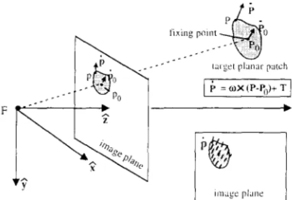
Let us see the configuration shown in Fig. 1. An MRPP in 3D space projects an optical flow field on the image plane (see the lower-right comer of Fig. 1). Its plane equation is

m x P x + m~.Py + m z P z :- m . P = d. (1) Here the symbol " . " denotes the inner product of vectors.

P = (Px, P y , P z ) T is a point on this planar patch. The image point of P is denoted by p = P / P z = (Px, Py, 1)T (perspective projection). Its optical flow vector is written

by p = (abx,]Ty,0) T.

The instantaneous 3D motion of this MRPP can be represented by d - ~ P = c v × ( P - P o ) + T . (2) . % fixing pnint

talget planar patch

[ ,; = o,× (,,-<)+ T]

L.

image plane Fig. 1. An optical flow field projected by a rigid moving planar

patch in 3D space.

The symbol " x " denotes the outer product of vectors, a: and T are instantaneous rotation and translation vectors (3 x 1). P0 = (Pox, P0r, P0z) T is a specially chosen point on the MRPP, whose image point and optical flow vector are separately denoted by p0=(P0x,P0y, l) T and li 0 = ~b0, ,/50y , 0) T. Without loss of generality, the global coordinate system is defined to be the same as the camera coordinate system given above.

Now we will introduce the concept of camera fixation. Let us see the configuration shown in Fig. 2 and compare it with that in Fig. 1. The old camera is now rotated (around its own focal point F) to a new pose R with an instantaneous rotation velocity ~2 in order that the new image point of Po is now kept at the image center (0,0) and its new optical flow vector is also kept to zero.

Here the 3 x 3 pose matrix R is defined as [Ul l u2 l u3].

{ui}s are three 3 x 1 orthonormal vectors. The time derivative of ui is lii = f~ × fii. The coordinate transform between the old camera system and the new one is represented by

P = R Q , (3) A point P seen by the old camera system is now renamed as Q in the new camera system.

The same MRPP in 3D space projects a new optical flow field on the new image plane (see the lower-right

Q fixing point ~ Q 0

H,

U~

target planar patch

standard tq{)w field

image plane

Fig. 2. By the process of camera fixation (rotating around its own focal center F), the input flow field p given in Fig. 1 can be transformed into its standard form /1. We call it standard

(3)

What can be seen in a noisy optical flow field? 1403

comer of Fig. 2). The plane equation seen by the new camera system is

nxQx + n r Q r + n z Q z ~ n . Q : d. (4) Here n = R T m . The image point of Q is denoted by q = Q / Q z = (qx, qy, 1) T (perspective projection). Its optical flow vector is written as /i = (q~, qy, 0) T. According to the definition of camera fixation, the two constraints, qo - (0, 0, 1)T and/i0 = (0, 0, 0) T, must be satisfied.

Now the instantaneous 3D motion of the MRPP seen by this new camera can be represented by the following special form:

Q = w* × (Q - Q0zz) + Tzz, (5)

where ~ = (0, 0, 1)T; Qoz is the Z-component of Qo; w* is a new 3 × 1 rotation vector; T~ is a 1 × 1 translational component.

In addition, several important transforms are listed below. To improve the reading, we neglect all of their details and show their final results only:

• Image point. The transform relationship between p and q is

q : . = (u2 p)/(u3 p) . (6)

1

• Optical flow. The transform relationship between !~ a n d / i is

Ii

i~1= - - u3 ' p [ a × ( R p ) + RI~]. 0 - ( u l ' p ) / ( u 3 " p ) ] 1 - ( u 2 p ) / ( u 3 " p ) 0 0 (7)

• 3D motion parameters. The transform relationship between {w,T} and {w*, Tk} is

w = R w * + f ~ ; T = T z u 3 + Q o z ( ~ 2 × u 3 ) . (8) From equations (6) and (7), we know that the new image points qs and their new flow vectors ilS can be directly generated by the old ps and liS once the pose matrix R and instantaneous rotation 9/of the new camera are given. We call {q,/i} the "standard form" of {p, p}.

2.2. Determine the required parameters f o r camera fixation

In order to transform the old flow field into its standard form, R and 9/ should be appropriately chosen for satisfying q0 = (0, 0, 1) T and/i0 = (0, 0, 0) T. We finally obtain the following results:

• Pose matrix R. The choice of R is not unique. We list one solution here:

u3 = Po/llPoll,

u2 = (Po × i ) / ( l l P o × ~'11), (9)

U 1 : U 2 × U 3 .

• Instantaneous rotation fL Substituting the constraints of q 0 = ( 0 , 0 , 1 ) T and / i 0 = ( 0 , 0 , 0 ) T into equation (7), the instantaneous rotation ~ must satisfy

9/:(-u2 P° ul ( P° u2

• ~ ) + \ u x . ~ ) + p u 3 .

(10) Here p can be any real value. We usually set p to zero for simplicity.

From equations (9) and (10), Po, and li 0, we can easily determine the required parameters (R and F0 for camera fixation. In fact, mechanically rotating the camera ac- cording to the solved R and C/is completely unnecessary! The standard flow field {q,/i} can be mathematically generated by using equations (6), (7) and (10).

The description of how to transform any optical flow field into its equivalent standard form is now complete.

2.3. Parameterization o f a standard f l o w field

Seen by the fixating camera, the flow field projected by a an MRPP in 3D space can be expressed by six coefficients {ai] i = 1 , . . . , 6} as follows:

[/L] [ a , q Z + a 2 q x q v + a 3 q x + a 4 q y ] ( l l )

ily = L a2q~ + a,qxqy + asqx + a6qy I '

where the flow coefficients ais are defined as

al =- w; - n;T~z, a2 =- -~*x - n;Tz,

a3 : --w;nrx -- T~z, a4 =- -~c;n' v - w~, (lZ)

* / * * / t

a5 =--~Cxnxq-~ z , a6 - - w x n y - T ' z,

T~ = T } / Q o z , ' - - * and (nx,nv) : (nx, ny)/nz. ' i The values, {a3, a4, as, a6}, defined in equation (12), are called the first-order flow coefficients, a~ and a2 are called the second-order flow coefficients. These coefficients can be easily solved by applying a linear regression method to the standard flow field.

The details of derivations of equations (11) and (12) are not given here. Readers may check them in references (1,2).

3 . M A I N A L G O R I T H M

If {w*, T~ } can be solved by using the flow coefficients ais, it is easy to transform these 3D motion parameters to the old ones {w,T} via equation (8). Therefore, without loss of generality, we only analyze the standard form of the flow field described by equation (11).

3.1. Motion estimation from first-order f l o w coefficients

When measuring the flow coefficients, the higher- order coefficients are always much more error sensitive than the lower-order coefficients. However, a complete solution of 3D unknowns requires the information of these higher-order coefficients. It means that the 3D estimates may not be robust enough. What can be gained if we only use the first-order flow coefficients? This topic will be discussed here.

(4)

1404 S.-C. PEI and L.-G. LIOU Let us define a 2 x 2 matrix A as

[

J[ ...

]

A ~ a3 a4 - ~ y n x - T~ - c o y n y - coz

(13)

= * l * , * l ! •

a5 a6 wxnx + coz ~ n y - T' z

By singular value decomposition (SVD), the matrix A can be rewritten by

where At _> A2 and At > 0. U a n d Vare 2 x 2 orthogonal matrices satisfying

From equation (2), A can be further decomposed into the sum of two matrices Aj and A2, where

[ Oqt

at2 ]

At =--/~2UV T ~

LO~2I OQ2J

(16)

A2 ~ (At - A2)uIvT ~ [fill fl12 ]

Lfl21 fl22

J

It is easy to find that the matrix At is a scaled orthogonal matrix and matrix A2 is not of full rank (rank=l, when At ¢ A2).

Besides, from equation (13), A can also be written as the sum of two matrices, B1 and B2, which are defined

as

L (co~

- k2)

[ - G ¢ ' , - k,

B 2 = * ' k

L

Wxnx+ 2

Here, kt and k2 are any two

that the matrix

n t

is also a

like A i.

-- (co; -- k2) 1

- ( r ~

k,);J

(17)

* Ht -- ] --co), y 1~2 c G n ;, - k t "

real values. It is obvious scaled orthogonal matrix If we wantAt = B1 andA2 - B2, what rules should kj and k 2 obey? It is clear that the determinant of B2 must be zero, just like that of A> After some mathematical manipulations, we find that kt and k2 must be on a circle characterized by

[kt + (fltt :~22-)J2--[k2

~ (/~1

2 / ~ 2 ) 2 ~

r 2.

_(~8)

Notice that this circle also passes through the origin (0,0). Therefore, (kt,k2) can be represented by a 0-parameter

family: (kl,kz)=(ktc,k2c) + r(cosO, sinO), where 0

ranges from 0 to 2r<

From equations (16)-(18), we have

jr) = _oq t + k t ,

* t =/~2t--k2,

cox nx , ! coynx = - - f i t t -- k l ,

adz ~ O~21 -}- k2~

cox'

ny

= fl22

nt- kl, co;n' v = -fl12 - k2. (19)

We may further separately define two new variables, h~ and h~, as the amplitudes of coxy (-= [ ~ , ~.]T) and n'xy

(_= [n'~, 4]~).

' ' (20)

~ y = h ~ y ; n~, =- hnn~y,

where ~ y and n~, are unit vectors.

After considering equations (18)-(20), it is easy to find that the value h~h, is independent of kt and k2:

h =_ h~h, = AI

-/~2

~ 0. (21) Substituting the 0-parameter expression of (kl,k2) into equation (19), we have

IT)

[ (~lt -- (f2~ll

+fl22)/21 + r c o s 0 ]

co*] =

[ [ct21 -- (flt2 -- f l 2 t ) / 2 ] + r s i n O J

I';l r c° °l

-= _co~¢ + L sin0 (22) w~ J \ L sm T2 J (23) where r l = [ 0 ~ + 7 r ] / 2 , r 2 = [ - 0 - ~ ] / 2 , c o s ~ - (-f~l, + & 2 ) / ( Z r ) , s i n ~ = (gt: + & t ) / ( Z r ) , s = ± l ,

and the sgn{. } function is especially defined as

1 i f x > 0 ,

sgn{x(0)} - - 1 if x < 0, (24)

s g n ( x ( 0 + A ) ) if x = 0 . The value of A is a very small positive number.

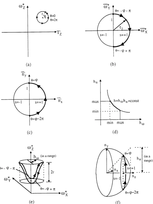
From equations (21)-(24), we have the following conclusions (only the first-order flow coefficients are used):

• The locus of (T), cv~) (as a function of 0) forms a circle with center (T),, co~<) and radius r. To any assigned value of 0, there is a corresponding unique solution for (T),a~,~). The circle shown in Fig. 3(a) is called the constraint circle for (T), or,).

• The locus of the unit vector ~xy (as a function of 0) is composed of two opposite half-circles ( s - ± l ) which completely occupy the whole unit circle [see Fig. 3(b)]. The unit vector n~y has a similar behavior [see Fig. 3(c)]. For any assigned value of 0, both wxy and Kxy are determined to a common sign s (=+1). • Although h~ and h, have not yet been completely

solved here, we know the value of h, which is defined as h~h,. Equation (21) indicates that h,(h~) will be easily obtained once giving h~ (h~). In fact, h~ (or h~) is usually of finite value. For example, it is impossible for an MRPP to move in 3D space by an infinitely large 3D rotation. Besides, the case that h,,=cxD is not acceptable because the projected image of the MRPP is now reduced to a line segment. Both h~ and h, should lie in some finite range [see Fig. 3(d)]. There- fore, as illustrated in Fig. 3(a)-(d), the possible 3D locus of ~* (or n) must also occupy a limited region in and

(5)

What can be seen in a noisy optical flow field? 1405 (0 Z

@

0---o

0=2x

' T z

(a)

I

s=- 1

n'x

(c)

(b)

h

n m a x

rain

~

hn=const

rain max

hm

(d)

CO Z (in a range) 0 = - q) - rt j I ( D y

0=-qo + rc

-~CO X ny / I \ - ~ '

h

/

(i.

~ ~ 0 = q ~ - 2 7 z

(e)

(t3

Fig. 3. The uncertainty of 3D motion estimation from the first-order flow coefficients.

3D space. Figure 3(e) shows a hollow cylinder which contains all of the possible values of a:* (a twisted, closed 3D slice). The height r and radius h~ of this cylinder are controlled by the difference of the two singular values, A1 and A2. In a similar way, Fig. 3(f) shows a circular band on a unit hemisphere, which indicates all of the possible directions n of the planar patch. From Fig. 3(a)-(f), readers can see how the

uncertainty of 3D estimates can be expressed quantitatively when using only first-order coefficients. • Without the information of the second-order flow

coefficients, the whole set of 3D motion/pose estimates are in fact a family of two unknown variables, 0

and h~. The inherent depth indeterminacy

Qoz

in a

monocular vision system is not considered here. Therefore, from the above results, only partial 3D

(6)

1406 S.-C. PEI and L.-G. LIOU

information can be recovered from its first-order flow coefficients.

3.2. Motion estimation from second-order flow

coefficients

Section 3.1 concludes that the 3D motion/pose of an MRPP in 3D space cannot be uniquely solved by its first- order flow coefficients only. If its second-order flow coefficients are used, can we obtain an unique solution? This topic will be discussed here.

From the definitions of al and a2 in equation (12), we have

I

w~.=,

-nxT

"]IJ II

) _ ,

I h~ = al (25)

w~ -nyT)

h,

a2

and

[ I

h~, 1 I T ) (

aln,, +

, a2n ,J

hn

-T)(wvny + aJxnx) L a2W'y + alWx

(26) Because the constraint of equation (21), that is

h~h~ = h,

must be satisfied, we may substitute

equations(26) and (19) and

(ka,k2)=(klc,k2,.)+

r(cos 0, sin 0) into equation (21). It finally becomes a third-order polynomial of z (=cos 0)

f ( z ) = - z 3 +

( ~ ) Z 2 + ( - I a~+a2"~

if2

) Z - -

e2 = O,

(27) where fill + fl22

e I = _ _

+oql ;

2 (28)

t/a2 - a2",~

{ala2"~ .

e 2 = ~ ) c ° s ~ P + ~ 2 ~ 5 - r 2 ) S m ~ + ( e f l ) •

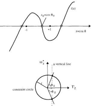
Let us see Fig. 4(a). Although the polynomial f l z ) = 0 has theoretically three roots for z, there is usually only

one root, say

z=zo--cosOo,

which can satisfy

- 1 < z < 1. To a value Zo, the angle 0 described in

equation (22) can be either 0o or 00. Let us see

Fig. 4(b). Solving f(z)=0 is equivalent to drawing a suitable vertical line through the constraint circle of (T),w~) to find its two intersecting points. Readers may compare Fig. 4(b) with Fig. 3(a) to check the definition of 0.

To each one angle of 0o and -0o, we know that Wxy and ' can be determined to a common unknown sign change

nxy

(s=4-1) by equation (23). Without loss of generality, we may let s = + l and substitute them into equation (26) to solve h~ and h,. In fact, we can always obtain the same

solution for

Wxy

and ffxy [defined in equation (20)] no

matter s = + 1 or - 1. Then a complete solution for n' (or n), w*, and T~ can be obtained.

Finally, we conclude that there are usually two ambiguous solutions for the motion/pose of an MRPP in 3D space if all of the flow coefficients (up to second order) are available.

f(z)

=-

,

~

Z=COS 0

constraint circle

Fig. 4. (a) The third-order polynomial

f(z)

obtained by the

second-order flow coefficients. Only the root inside [ 1,1] is accepted. (b) Solving f(z)=0 is equivalent to drawing a corresponding vertical line on the (T~,w~) plane and then finding its two intersecting points on the constraint circle.

While using equation (27), the case that r = h = 0 will make equation (27) unusable and we have to consider equation (25) again. Even so, we still have two solutions:

h "

*

(1) If h~, 0 (t at IS, wx~. = [0, 0]v), the vector n]y is

T t "

equal to - [ a l , a2]

/T).

(2) I f h , = 0 (or n'~,. = [0, 0]T), ' * is equal to [--a2, all T.

the vector w

4. DISCUSSIONS

In this section, we would like to make a global description about what can be seen in a noisy flow field projected by an MRPP. It is hoped that the readers can get a clearer picture to this problem.

4.1. Parameterization of noisy flow measurement

Our analysis is totally based on the coefficients of the (standard) flow field. These coefficients can be determined from various sources: (1) the optical flow estimated by the so-called gradient-based methods, (2) the normal flow estimated by moving image contours, ~L2) (3) the displacement vectors estimated by the so-called block-matching or correlation-based methods; the discrete-time image measurement is now an approxima- tion of the continuous one. No matter where these coefficients come from, our analysis can be directly applied to them.

The most important reason for us to adopt flow coefficients as basic measures is the requirement for reliability. Due to the redundancy of input data, the accuracy of flow coefficients is much better than that of individual image points and optical flow vectors. So

(7)

from first-order coef.

f.O*

z vertical line

from second-order coef.

tainty region

constraint circle

I~ T' z

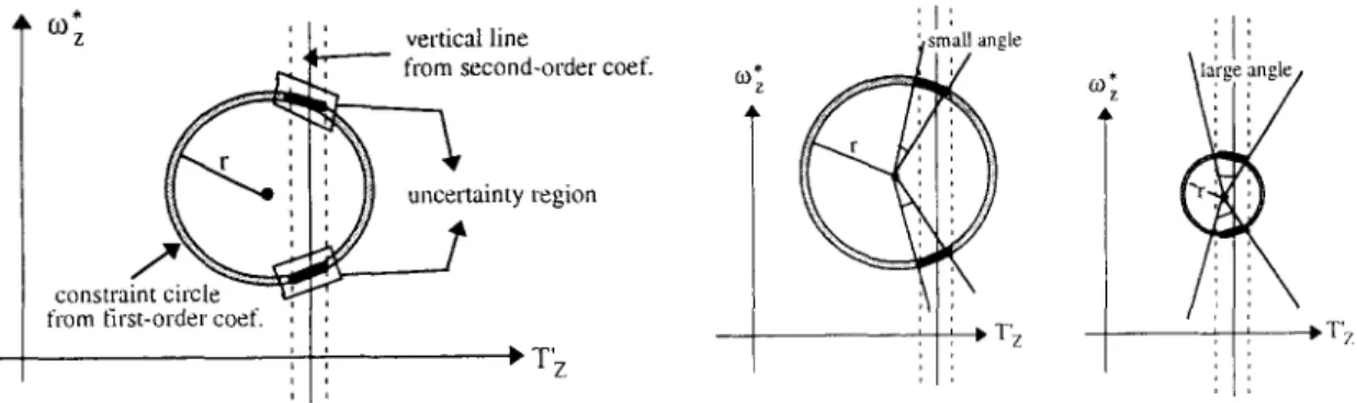
Fig. 5. The uncertainty region of a noisy flow field (for its 3D estimates) is determined by the intersection of two areas: (1) the possible perturbation range of the vertical line, (2) the

possible perturbation range of the constraint circle.

03' :1:

~

mall angle ; ; ,~T' z \ la'rg!

7

T' z

Fig. 6. Trade-off between the accuracy of 3D estimates. Same perturbation range of T~ will induce different error performance for the cases having different radius r. Smaller radius r implies smaller perturbation to ~ , but larger perturbation to

the direction of u:x~.

the accuracy of 3D estimates will be improved without any question.

4.2. Uncertainty of 3D estimates

From Section 3.1 and Fig. 3, we know that the SVD of A dominates our interpretation to 3D motion/pose. The most important quantity is the difference between singular values, A~ - A2. It specifies the size of uncertainty when we only consider the first-order flow coefficients. From Section 3.2 and Fig. 4, it is straightforward that solving the SFM problem is just equivalent to drawing a vertical line through the constraint circle of (T~, ~;*) to find its two intersecting points. The constraint circle is estimated by the four first-order coefficients only, but the vertical line is estimated by the second-order ones. Because the second-order flow coefficients are usually much more error-sensitive than the first-order coefficients, the positional perturbation of the vertical line (due to noise) is often larger than that of the constraint circle. Figure 5 illustrates the above idea. So the final 3D estimates from a noisy flow field must fall into an uncertainty region specified in Fig. 5, whose size de- pends on the amplitude of noise.

On the other hand, a quantity called impacting time,

denoted by tim p here, is just equal to

1/T~

defined in this

paper. Readers should notice that both of the two ambiguous solutions have the same value of tim p. It means that we will always have a unique estimate for timp, no matter how many ambiguous solutions are obtained. The size and position of the uncertainty region shown in Fig. 5 is directly related to the maximum and minimum range of timp, which can be used as the basis of obstacle avoidance in an auto-vehicle's vision system.

Some readers may think that a smaller constraint circle for (T~, w*) often implies a smaller uncertainty for 3D estimates. But it is wrong! Let us see Fig. 6 for further explanation. The same perturbation of the vertical line induces different results: smaller radius r means smaller variance for T~ and ~ , but larger variance for the

directions of

W~y*

and n'xy. It is because the uncertainty

regions for both cases occupy different ranges of 0 which are directly related to the uncertainty of ~o~. and nxy

according to equation (23). It seems that there is a "trade-off" between the accuracy of different 3D estimates.

5. EXPERIMENTS

In this section, several sets of experiments are designed for testing our algorithm. They have three goals: (1) To prove the correctness of the algorithms (simulated image). (2) To show the tendency of error sensitivity when the relative poses of the target planar patch are varied in a controlled manner (simulated image). (3) Our analysis is workable in the real-world application (real- world image).

Before describing these experiments, there are two things to be noticed:

• All the planar patches tested in Sections 5.1 and 5.2 are the same. It is a 3 x 3 square patch with 25 uniformly-distributed feature points. Its central point, the 13th feature point, is the specially chosen fixing point Po. Parameterization of the given flow field is totally based on these 25 feature points and their optical flow vectors. In order to verify the correctness of our algorithm, the flow vectors in computer simula- tions are generated by a simple, well-known physical rule: o.2)

Here [~ is generated by the definition given in equation (2).

• In Section 5.2, the noisy flow field is generated by

purposely adding a 2D random noise

(nl,n2)

on the

error-free flow field like this

error_perturbed [~:1 = [~;i] + I n : ] . (30)

Here n~ and n2 are random variables of normal dis- tribution N(0,cr) and

(8)

1408 S.-C. PE1 and L.-G. LIOU

The p e r c e n t a g e ratio ~ is defined as the noise level. For simplicity, other possible error sources such as quantization errors, c a m e r a calibration errors, and fixation errors are a s s u m e d to be error-free throughout the e x p e r i m e n t s in Section 5.2.

5.1. Error-free experiments

Figure 7(a) shows an optical flow field li projected by an M R P P in 3D space. T h e true 3D m o t i o n / p o s e o f the M R P P is r a n d o m l y assigned. By equations (9) and

I

-08;

L'

-0.2 ~ -0.2 o--

J

I

o" o- °,~o

0 0 ~ ~ o r . ~ ' ~ ., -

i

-0.5 0 0.5 -0.5 0 0.7i 0.6 05 0.4 (a) f o z " r l 0 0.2 ( c )

(b)

COy

L

o (

-I fO x

i

0 ( d )

X

-I

x

6

( e ) 6 5 .... i ... i ... ~, ... 4 ... i ... i ... 3 ... i ... i ... 2 .... i ... i ... 0 ... i ... 1 -1 0 1

Z taCOs 0

( g ) 1.5 I 1 0.5 ht~

012

014

( t )

Fig. 7. Several plots of the results obtained in the error-free experiments. 0.5

(9)

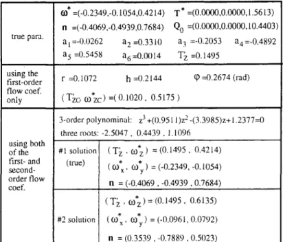
What can be seen in a noisy optical flow field? 1409 true para. using the first-order flow coef. only using both of the first- and second- order flow coef. =(-0.2349,-0.1054,0.4214) n =(-0.4069,-0.4939,0.7684) a 1 =-0.0262 a 2 =0.3310 a 5 =0.5458 a6 =0.9A)14 T * =(0.0000,0.0000,1.5613) Qo =(0.0000,0.0000,10.4403) a 3 =-0.2053 a 4 =-0.4892 Y~ =0.1495 r =0.1072 h =0.2144 q) =0.2674 (rad) ( T~o CO zc) =( 0.1020, 0.5175 ) * 3-order polynominal: z 3 +(0.951 l)z 2 -(3.3985)z+ 1.2377=0 three roots: -2.5047, 0.4439, 1.1096 #1 solution (true) ! #2 solution ( T ~ , COz ) = (0.1495, 0.42t4) ( CO*, COy ) = (-0.2349, -0.1054) n = (-0.4069, -0.4939,0.7684) ( T ~ , CO z) = (0.1495, 0.6135) (cox' COy) = (-0.0961, 0.0792) n = (0.3539, -0.7889,0.5(123) Fig. 8. The results of the error-free experiment.

(10), this flow field is then changed into its standard form shown in Fig. 7(b). Notice that the flow fields shown in Fig. 7(a) and (b) have been suitably scaled (0.3 and 0.5) for a better look. The first part of the table in Fig. 8 lists: (1) the true 3D motion/pose of the MRPP seen by the rotated camera, (2) the true flow coefficients of the standard flow field shown in Fig. 7(b).

If we only consider the first-order flow coefficients, only partial information can be recovered. The second part of the table in Fig. 8 lists all of the solved quantities. Figure 7(c) plots the solved constraint circle. It is easy to

check that the true

(T~,w~)

(denoted by " * " ) is lies

exactly on this circle.

Figure 7(d) and (e) show the possible values of ~3xy and n~.. Two opposite half-circles (solid for s = + 1 and dotted for s = - 1) occupy the whole unit circle. If the true angle 0 is given and substituted into equation (23), we will obtain its corresponding C0xy and n~y (represented by a dotted straight line through the origin). It is easy to check that the true solutions (marked by " * " ) are just lying on the straight lines, which proves equation (23). Figure 7(f) shows the uncertainty of h~ and h,,. The true solution (marked by " * " ) is just lying on this curve, which proves equation (21).

If the second-order flow coefficients are considered, we will have two ambiguous solutions. Figure 7(g) shows the third-order polynomial function,f(z)=0. It has three roots: z=cos 0 = { - 2 . 5 0 4 7 , 0.4439, 1.1096}. Only the second one satisfies the constraint [z[ _< 1. So we have two ambiguous solutions listed in the third part of the table shown in Fig, 8. Notice that the first solution is just equal to the true solution. It proves our algorithm.

5.2. Analysis of error sensitivity

To analyze the error sensitivity of the 3D estimates, five cases are defined here. All of the MRPPs tested in these cases have the same point Po located at (0, 0, 10) v and the same 3D motion: ~ = (0, 0.5, 01 T, translation T = (0, 0, 2) T. The normal vectors of these five MRPPs

can be represented by the following form:

m = (sin a, 0, cos a) T. From cases 1-5, their corresponding angle c~s are separately set to 0 °, 15 °, 3if, 45 °, and 60 °.

For the above five specially-designed testing cases, all of their generated flow fields have been standardized and hence we can directly ignore the process of

camera fixation. So a ; = w * , T = T * , m = n , and

T.~ = 2 / 1 0 = 0 . 2 .

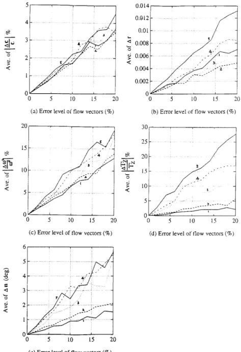
Figure 9(a)-(e) show the error performance of the five cases for noise level 6 ranging from 0% to 20%. Each point on the curves is the average of 100 tests. Figure 9(a) and (b) shows the results when only the first- order flow coefficients are considered. Figure 9(a) shows the position error, ][AcH/]]c]], of the center c of the constraint circle. Figure 9(b) shows the deviations A r of its radius r. The radii r of the five cases are: 0, 0.0551, 0.1443, 0.2500, and 0.4330. We find that the estimate of the constraint circle is very robust. Besides, it seems that the different orientations of a planar patch do not affect the error sensitivity of the uncertainty estimate remarkably.

Figure 9(c)-(e) show the results when the second- order flow coefficients are considered. Because there will be two ambiguous solutions, we choose the one nearest to the true solution as our estimate. Figure 9(c)

(10)

1410 S.-C. PEI and L.-G. LIOU < 4

3 i

i

.i '

" 2 ~ ' "" <" " " 1 0 0 5 I0 15 20 0.014 ,- i ' 0.012 b ...

0.0, F

. . . . . . . / . . . .

:

5o o.oo V

. . . . . . 0.0061- ... ~ ... ... :-~ - < t " ~ i . . . . . 0.004 0 5 10 t5 20

(a) Error level of flow vectors (%) (b) Error level of flow vectors (%)

20 . ~ , , 30 - ,

15 . . . .

o J'

. . .

' ...

J"

0 5 10 15 20 0 5 10 15 20

(c) Error level of flow vectors (%) (d) Error level of flow vectors (%)

< 6

5

... i . . . , ... i ... , . ,

4

... ! . . . i . . . ,./~-!.•::i :i_ 3 ... ... ..:..:-.-! :::: :: .... 2 ... ...~;!.: y . . , i < . . ,.... i ... 0 0 5 l0 15 20

(e) Error level of flow vectors (%)

Fig. 9. Analysis of error sensitivity.

the rotation a J*. Figure 9(d) shows the estimation errors,

d e f i n e d as

][AT~II/IT~[,

o f the translation T = (0, 0, Tz).

Figure 9(e) shows the estimation errors, A n , o f the normal vector n. We find that the estimates obtained from a more-slanting planar patch are m o r e error sensitive than those f r o m a less-slanting one. This t e n d e n c y is especially remarkable in Fig. 9(d) w h e n estimating the translation. No doubt, the error p e r f o r m a n c e o f the estimate o f T~ will affect the error p e r f o r m a n c e s o f the other estimates such as u;* and n. It is because ~ y and n are d e t e r m i n e d after w e know the value o f z (or T~). Although there is a t e n d e n c y that a larger radius r (of the constraint circle) usually induces a smaller error sensitivity in estimating the directions o f 03, o. and n'~, the t e n d e n c y s h o w n in Fig. 9(d) s e e m s m u c h stronger and then dora-

inates the later error p e r f o r m a n c e s s h o w n in Fig. 9(c) and (e). Notice that the differences a m o n g the curves in Fig. 9(c) and (e) are not so obvious as that in Fig. 9(d).

5.3. Real-image experiment

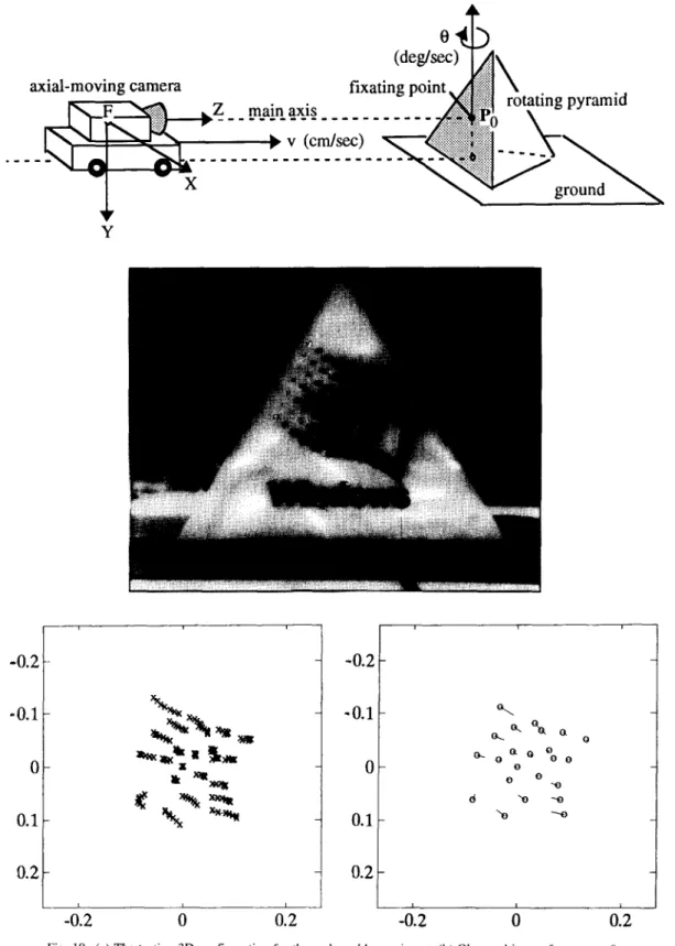
To test the p e r f o r m a n c e o f our algorithm in a real application, we d e s i g n e d a simple and well-controlled e x p e r i m e n t in our laboratory. A planar patch m o u n t e d on a p y r a m i d - t y p e object is c o n s i d e r e d [see Fig. 10(a)]. E a c h one o f the four sides o f the p y r a m i d - t y p e object is an equilateral triangle. For c o n v e n i e n c e in 3D measurement, the relative 3D m o t i o n b e t w e e n the c a m e r a and the plate is controlled by two parameters: a Z-direction translation Vz ( - - 2 7 . 5 cm/s) o f the camera, and a rota-

(11)

(deg/sec

axial-moving camera

fixating point ~ i i J \

,~Z

main axis

~ 1

rotating pyramid

. . . . " . . . . " . . . ...::::, • .0 v. V ( c m / g e c ) I~ ..:.:.:.::::::!:!:i:!~i!!¥ii~i~;!!!~: ~ i i l . . ~ " ~

Y

-0.2

-0.1

0

0.1

0.2

II, ~11

-0.2

-0.1

0

0.1

0.2 o...

a . % a

O.. 0 0 o 0 0 . . . .

12 -0.2

0

0.2 -0.2

0

Fig. 10. (a) The testing 3D configuration for the real-world experiment. (b) Observed image frame at t=0. The white dots denote the selected feature points on the plate. (c) The point trajectory of every selected feature point in the image sequence (of 7 frames). (d) Estimated flow vector at t=0. Scale of the flow vector

is set to 0.5.

tion 0 ( = + 6 0 ° / s ) around the Y-axis which passes through a chosen fixed point Po on the plate. At t=0, the 3D coordinate of Po is (0, 0, 109.8 cm); the plane equation of the plate is ( 1 / 3 ) Y + ( 2 x / ~ / 3 ) Z = ( 2 x / 2 / 3 ) . 109.8 cm.

The CCD camera has been calibrated by a simple pin- hole model. The resolution of the image plane is 512 × 480 (pixels); viewing angle is about 30°; the focal length is about 18.3 cm.

(12)

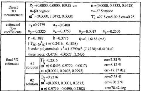
1412 S.-C. PEI and L.-G. LIOU Direct 3D measurement PO =(0.00(~, 0.0000, 109.8) cm 0---60 deg/sec =(0.0000, 1.0472, 0.0000) n =(0.0000, 0.3333, 0.9428) v=-27.5cm/sec T~ =27.5 cm/109.8 cm=0.25 estimated a I --0.9779 a 2 --0.0400 flow

coefficients a 3 =-0.2325 a4 =-0.3753 a5=-0.0017 a6=-0.2506

final 3D estimates r ---0.1887 h ----0.3775 q~ --0.1.6188 (rad) ( T ~ , O)zc)* =(0.2416, 0.1868) 3-order polynominal: z3+(1.2799)z 2-(7.7228)z-0.4101--0 three roots: -3.4709, -0.0527,2.2436 T~ --0.2316 #1 • solution cO =(-0.0493, 0.9779, -0.0017) n =(0.0001, 0.0402, 0.9992) err=7.35 % err=8.12 % err=17.17 deg T~--0.2316 #2 solution 0.1'=(0.0093, 0.0001, 0.3573) n =(-0.9719, -0.0490, 0.2302) err=7.35 % err= 106.2 % err=78.42 deg Fig. 11. Experimental results of the real-image test.

In order to estimate the instantaneous flow vectors at t--0, an image sequence of seven image frames ( t : - 0 . 5 , - 0 . 3 3 , -0.167, 0, +0.167, +0.33, +0.5 s) is taken. Figure 10(b) shows the observed image at t=0; 23 white dots denote the selected feature points on the plate. After finding the corresponding feature points at each time instant, the trajectory (x(t),y(t)) of every feature point (x(0),y(0)) is fitted by a third-order polynomial model:

(x(t), y(t) ) = ( ~ = 0 Cxiti' ~']~=0

CY iti)"

Therefore, the flow vector (k(0), ~(0)) is estimated by (Cxl,Cyl). Figure 10(c) shows the point trajectory; Fig. 10(d) shows the estimated flow vectors. Notice that the length unit of image coordinates in Fig. 10(c) and (d) has been changed from one pixel to one focal length.

Figure 11 lists the final 3D estimates. The #1 solution is quite close to our true 3D measurements. Large magnitude of estimation errors are reasonable because of the errors from (1) camera calibration, (2) image quantization. Besides, the small viewing angle of the object does increase the error sensitivity.

6. CONCLUSION

In this paper, we propose a new algorithm to solve and analyze the SFM problem from the optical flow field projected by an MRPP in 3D space. Although our approach has exactly the same solution just like the old approaches did before, there are several additional advantages of our algorithm: (1) It is very easy to analyze the error sensitivity, ambiguity, and uncertainty in a noisy optical flow field. (2) Our algorithm introduces the concept of camera fixation and reduces the number of parameters while representing a flow field (from eight to six). (3) The SFM problem can be solved by "levels." According to the accuracy of observed flow field, we can interpret the flow field from coarse to fine (from constraint circle to two ambiguous solutions). (4) Our derivations clearly show the trade-off

of accuracy when solving the 3D motion/pose parameters.

To analyze the SFM problem more completely, several experiments are designed. We draw the following conclusions: (1) When using first-order flow coefficients only, the estimate for the constraint circle is quite error insensitive. (2) When using full information of flow coefficients, the estimate is usually error-sensitive. (3) The tendency of the error performance with respect to different orientations is shown.

What can be seen in a noisy flow field projected by an MRPP in 3D space? Finally we can say: " Much more than just obtaining two ambiguous solutions."

REFERENCES

1. A. M. Waxman and K. Wohn, Contour evolution, neighborhood deformation, and global image flow: Planar surfaces in motion, Int. J. Robotics Res. 4(3), 95-108 (1985).

2. A, M. Waxman and S. Ullman, Surface structure and 3D motion from image flow kinematics, Int. J. Robotics Res. 4(3), 72-94 (1985).

3. K.-I. Kanatani, Detecting the motion of a planar surface by line and surface integrals, Comput. Vision Graphics Image

Process. 29, 13-21 (1985).

4. R. Y. Tsai, T. S. Huang and W.-L, Zhu, Estimating three- dimensional motion parameters of a rigid planar patch 1I: Singular value decomposition, 1EEE Trans. Acoust. Speech

Signal Process. ASSP-30(4), 525-534 (August 1982). 5. R. Y. Tsai and T. S. Huang, Estimating three-dimensional

motion parameters of a rigid planar patch III: Finite point correspondences and the three-view problem, IEEE Trans.

Acoust. Speech Signal Process. ASSP-32(2), 213-220 (1984).

6. R. Y. Tsai and T. S. Huang, Motion and structure from point correspondences with error estimation: Planar sur- face, IEEE Trans. Signal Process. 39(12) 2691-2716 (December 1991).

7. K.-I. Kanatani, Structure and motion from optical flow under perspective projection, Comput. Vision Graphics

(13)

8. K.-I. Kanatani, Tracing planar surface motion from a projection without knowing the correspondence, Comput.

Vision Graphics Image Process. 29, 1-12 (1985).

9. R. Mukundan and N. K. Malik, Attitude estimation using moment invariants, Pattern Recognition Lett. 14, 199-205 (1993).

10. T. Y. Young and Y.-L. Wang, Analysis of 3D rotation and linear shape changes, Pattern Recognition Lett. 2, 239-242 (1984).

11. R. Mukundan, Estimation of quaternion parameters from two-dimensional image moments, CVGIP: Graphical

Models Image Process. 54(4), 345-350 (1992).

12. S. C. Pei and L.-G. Liou, Tracking a planar patch in 3-D space by affine transformation in monocular and binocular vision, Pattern Recognition 26(1), 23-31 (1993). 13. S. C. Pei and L.-G. Liou, Finding the motion, position and

orientation of a planar patch in 3-D space from scaled- orthographic projection, Pattern Recognition, 27(1), 9-25 (January 1994).

14. C. A. Rothwel, A. Zisserman, C. I. Marinos, D. A. Forsyth and J. L. Mundy, Relative motion and pose from arbitrary plane curves, Image Vision Comput. 10, 250- 262 (1992).

15. J. C. Hay, Optical motion and space perception: An extension of Gibson's analysis, Psychol. Rev. 73, 550-565 (1966).

16. S. Negahdaripour, Closed-form relationship between the two interpretations of a moving plane, J. Opt. Soc. Am. A 7(2), 279-285 (February 1990).

17. H. C. Longuet-Higgins, The visual ambiguity of a moving plane, Proc. Roy. Soc. London Ser. B 223, 165-175

(1984).

18. S. Ullman, Optical Flow of Planar Surfaces. MIT Memo 870, Massachusetts Institute of Technology, Cambridge, Massachusetts (1985).

19. B. K. P. Horn, Motion fields are hardly ever ambiguous,

Int. J. Comput. Vision 1(3), 259-274 (1987).

20. S. Negahdaripour, Multiple interpretations of the shape and motion of objects from two perspective images, IEEE

Trans. Pattern Analysis Mach. Intell. 12(11), 1025-1039

(November 1990).

21. R. Y. Tsai and T. S. Huang, Uniqueness and estimation of 3D motion parameters of rigid objects with curved surface,

1EEE Trans. Pattern Analysis Mach. lntell. PAMI-6, 13-27

(1984).

22. H. C. Longuet-Higgins, Multiple interpretations of a pair of images of a surface, Proc. Roy. Soc. London Set A 418, 1-15 (1988).

23. C. Fermuller and Y. Aloimonos, The role of fixation in visual analysis, Int. J. Comput. Vision 11(2), 165-186 (1993).

24. Y. Aloimonos, I. Weiss and A. Bandyopadhyay, Active vision, Int. J. Comput. Vision, 333-356 (1988).

25. D. H. Ballard, Animate vision, Artif. lntell. 48, 57-86 (1991).

26. A. L. Abbott et al., Promising directions in active vision,

Int. J. Comput. Vision 11(2), 109-126 (1993).

27. J. K. Tsotsos, On the relative complexity of active versus passive visual search, Int. J. Comput. Vision 7(2), 127-141 (1992).

28. J. D. McDonald, A. T. Bahill and M. B. Friedman, An adaptive control model for human head and eye move- ments while walking, IEEE Trans. Systems Man Cybernet. SMC-13(2), 167-174 (March/April 1983).

About the A u t h o r - - S O O - C H A N G PEI was born in Soo-Auo, Taiwan, R.O.C., on 20 February 1949. He received the B.S. degree from National Taiwan University in 1970 and the M.S. and Ph.D. degrees from the University of California, Santa Barbara, in 1972 and 1975, respectively, all in Electrical Engineering. He was an Engineering Officer in the Chinese Navy Shipyard at Peng Fu Island from 1970 to 1971 and a Research Assistant at the University of California, Santa Barbara, from 1971 to 1975. He was Professor and Chairman in the Department of Electrical Engineering at Tatung Institute of Technology from 1981 to 1983. Presently he is the Professor and Chairman of the Department of Electrical Engineering at National Taiwan University. His research interests include digital signal processing, digital picture processing, optical information processing, lasers, and holography. Dr Pei is a member of the IEEE, Eta Keppa Nu, and the Optical Society of America.

About the A u t h o r - - L I N - G W O LIOU was born in Taiwan. He received the B.S. degree from National Chiao Tung University (N.C.T.U.) in Taiwan in 1989 and the Ph.D. degree from the National Taiwan University in 1995, both in Electrical Engineering. He is currently doing military service. His research interests include motion image analysis, methods for 3-D object reconstruction, and pattern recognition in image applications.