An intelligence system approach using artificial neural networks to evaluate the quality of treatment planning for nasopharyngeal carcinoma

(1)

Full Length Research Paper

An intelligence system approach using artificial neural

networks to evaluate the quality of treatment planning

for nasopharyngeal carcinoma

Tsair-Fwu Lee

1

*

#

, Pei-Ju Chao

1,2#

, Chang-Yu Wang

3,4

, Wei-Luen Huang

1

, Chiu-Ching Tuan

5

,

Mong-Fong Horng

1

, Jia-Ming Wu

6

, Shyh-An Yeh

6

, Fu-Min Fang

2

and Stephen Wan Leung

4

1

Medical Physics and Informatics Laboratory, Department of Electronics Engineering, National Kaohsiung University of

Applied Sciences, Kaohsiung, Taiwan.

2

Department of Radiation Oncology, Kaohsiung Chang Gung Memorial Hospital and Chang Gung University College of

Medicine, Kaohsiung, Taiwan.

3

Department of Electrical Engineering, National Kaohsiung University of Applied Sciences, Kaohsiung, Taiwan.

4

_{Department of Radiation Oncology, Yuan’s General Hospital, Kaohsiung City, Taiwan.}

5

Department of Electronics Engineering, National Taipei University of Technology, Taipei Taiwan.

6

Department of Radiation Oncology, E-Da Hospital /I-Shou University, Kaohsiung, Taiwan.

Accepted 30 May, 2012

The quality of the nasopharyngeal carcinoma (NPC) treatment plans evaluation using three types of

artificial neural networks (ANNs) are instructed by three different training algorithms. Three ANNs

including Elman (ANN

-E

), feed-forward (ANN

-FF

), and pattern recognition (ANN

-PR

) were trained by using

three different models, that is, leave-one-out (Train

-loo

), random selection (Train

-random

), and user defined

(Train

-user

) method. One hundred sets of NPC treatment plans were collected as the input data of the

neural networks. The conformal index (CI) and homogeneity index (HI) were used as the characteristic

values and also to train the neurons. Four grades (A, B, C, and D) were classified in degrading order.

The over-training issue is considered between the train data and the number of neurons. The receiver

operating characteristic (ROC) curves were obtained to evaluate the performed accuracies. The optimal

numbers of neurons for ANN

-E

, ANN

-FF

, and ANN

-PR

, in the loo method are 6, 24, and 9; in the

random-selection method, they are 26, 22, and 4; and in the user-defined method they are 12, 8, and 11 neurons,

respectively. The optimal size of train data is 92% of total inputs in the cases of ANN

-E

and ANN

-FF

and

76% in the case of ANN

-PR

. The networks with higher accuracy are ANN

-PR-loo

(93.65 ± 3.60%), ANN

-FF-loo

(88.05 ± 5.84%), and ANN

-E-loo

(87.55 ± 5.86%), respectively. The networks with shorter training time are

ANN

-PR-random

(0.55 ± 0.11 s), ANN

-PR-user

(0.59 ± 0.08 s), and ANN

-PR-user

(1.07 ± 0.16 s), respectively. The

ROC curves show that the ANN

-PR-loo

approach has the highest sensitivity, which is 99%. ANN

-PR-loo

reduces the amount of trail-and-error during the iterative process of generating inverse treatment plans.

It is concluded that the ANN

-PR-loo

is an excellent model among the three for classifying the quality of

treatment plans for NPC.

Key words: Artificial neural networks (ANNs), dose-volume histogram (DVH), intelligence system,

nasopharyngeal carcinoma (NPC).

INTRODUCTION

Clinically, intensity modulated radiation therapy (IMRT) is

the most common technique to deliver radiation doses to

nasopharyngeal carcinoma (NPC) patients, because

IMRT is capable of delivering a high dose to the irregular

tumors, and prevents organs at risk (OARs) and normal

tissues from being exposed to radiation. However, it is

usually difficult to complete a suitable IMRT plan at one

time because both the patient’s condition and some

complex formulas need to be considered simultaneously.

The IMRT technique greatly benefits NPC patients,

offering much higher treatment quality. The IMRT

technique combines several different radiation fields to

(2)

produce steep dose-volume histogram (DVH) and

isodose curves for the planned target. These steep

curves mean that the dose gradient at the border

between cancerous and normal tissue varies rapidly.

Usually the acceptable dose distribution can be produced

by using seven to nine fields (Lee et al., 2008; Oldham et

al., 2008).

A treatment plan that results in a higher planning target

volume (PTV) coverage and reduce the complications in

normal tissues is preferred, and this may be done after

several attempts using trial and error. The inverse

calculation is one kind of algorithm that is embedded in

treatment planning systems (TPS). It is generally used in

the optimization procedure for IMRT. The inverse

calculation adopts iterative operation and an optimal

algorithm to produce varied intensity of treatment beams.

This allows IMRT to find a dose that compromises

between the PTV and critical organs (Webb, 2004; Leung

et al., 2007). The interactive interface is also supported in

modern planning systems. The dose-volume based

weighting and the priority of the critical organs can be set.

Therefore, planners can define some limits for PTV and

OARs, which is called constraint-based optimization.

In order to find the solution during the optimization

procedure, three steps are performed: (1) determine the

constraints and priority setting making up an objective

function by the planner, (2) work out the objective

function, and (3) evaluate the quality of the treatment

plan with the prescribed dose and criteria. These three

steps are executed sequentially or iteratively until an

optimal solution is reached (Stieler et al., 2009).

However, the quality of a final plan depends on the

planners’ experiences, which may be learned from

others’ experience or published journals (Deasy et al.,

2007; Wilkens et al., 2007). It is very time-consuming for

a planner to fine-tune for individual optimal solutions.

Technically the final result obtained is usually not an

optimal solution, but a sub-optimal one. Generally, if we

want to find an optimal solution, we have to consider not

only a minimum objective function, but also the individual

clinical conditions and many parameters not included in

the objective function. If an expert knowledge-based

system is applied to learn and to accumulate those

experiences, then the time taken to create an optimal

treatment plan will be reduced. This knowledge-based

system is especially effective for complex treatment

plans, such as NPC plans.

Artificial neural networks (ANNs) are widely used in the

modern sciences (Wu et al., 2009; Bahi et al., 2006;

*Corresponding author. E-mail: tflee@kuas.edu.tw or lwan@ms36.hinet.net.

#Both author contribution equally. Part of this study was presented at the International Conference on Agricultural, Food and Biological Engineering (ICAFBE 2012)

Lee et al. 2077

Vasseur et al., 2008). There are some major researches

on ANN models that were used to predict the side effects

after radiation therapy. For instant, the leave-one-out

(loo), random-selection, and user-defined methods were

applied to train the feed-forward ANN model introduced

by Su et al. (2005) which is used to predict the probability

of pneumonitis after treatment. The sensitivity obtained

by the three different methods are 0.95, 0.57, and 0.71

and their respective accuracies are 0.94, 0.88, and 0.90.

The ANN is also used to calculate the probability of

developing radiation pneumonitis, as proposed by Chen

et al.

(2007). Based on Chen’s model, the receiver

operating characteristic (ROC) curves show that the

sensitivity is 0.67, the specificity is 0.69, p = 0.020.

Obviously, involvement of the aforementioned non-dose

characteristics

makes

ANNs

more

generalized.

Moreover, Mathieu et al. (2005a) adopts an ANN to

optimize the dose distribution. It is applied in treatment

plans to make sure the time taken for calculation is

acceptable and the error is less than 2%. Isaksson et al.

(2005) also uses the feed-forward network to predict the

motion of a tumor in the lung during radiation therapy.

Results show that this method is better than the

conventional one and the self-adaptive filter. Many kinds

of treatment techniques introduced by Bortfeld and Webb

(2009) are used to reduce the treatment time effectively.

Our preliminary result (Chao et al., 2010) shows that a

back-propagation model using dose parameters and

dose indices can produce high accuracy in evaluating

NPC plans. Some applications of ANNs were used in the

past to implement 3DCRT plans effectively and

efficiently, and a few of them were applied in the expert

system of IMRT.

Whether a treatment plan is acceptable or

unaccept-able, it usually depends on the planner’s experience. It is

time-consuming to evaluate the calculated results and

fine-tune the weightings by trial and error. In this study,

three types of ANNs are instructed by three different

training algorithms to effectively evaluate the quality of

the NPC treatment plans. A better match for ANN and the

training algorithm will be chosen and established. We aim

to help to make an intelligence judgment that reduces the

amount of interaction between planner and TPS during

the iterative process of generating inverse treatment

plans. It can decide whether a plan is acceptable and

ranking the quality of treatment plans automatically,

therefore, providing an improvement suggestion when the

plan was not acceptable.

MATERIALS AND METHODS

Three different neural network models, namely, the Elman (ANN-E), feed-forward (ANN-FF), and pattern recognition (ANN-PR) models, are adopted. Each model is worked with three selection methods, named the leave-one-out (loo), random-selection, and user-defined methods, to train the neurons. The overall system flowchart is as shown in Figure 1. The data of DVHs are imported into the untrained ANNs and the training method is selected. We want to

(3)

Treatment

planing

Manual

evaluation

ANN

Evaluation

system

Check

criteria

Ready for

delivery

Plan improvement

suggestions

Yes

No

Figure 1. System flowchart for plan quality evaluation and

improvement suggestions; ANN: artificial neural networks.

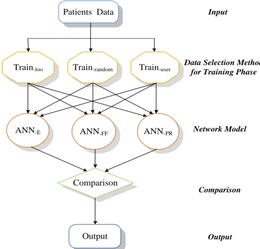
find an ANN model that matches a specific training method to produce the highest accuracy by consideration a mong the conditions of the training time, the number of neurons, the size of training data population, and ROC curves (Chen et al., 2007; Mathieu et al., 2005b). Then, the model can be taken as the best one to evaluate the treatment plans. The basic neural networks structure of the selection procedure is as shown in Figure 2. In the following, parameters and neural networks used are described.

Input parameters

According to the International Commission on Radiation Units and Measurements (ICRU) Report 62, the planning organ-at-risk volumes (PRVs) were defined as a safety margin around the OARs, particularly for a high-dose gradient area. In this study, the PRV of the spinal cord was determined by adding a 3D margin of at least 5 mm to the delineated spinal cord. The PRVs of the brain stem and chiasm were defined through addition of a 3D margin of at least 1 mm around the delineated structures. According to the suggestions of Radiation Therapy Oncology Group (RTOG) 0225 (Lee et al., 2003), one hundred NPC samples (NP = N100) are collected as the inputs, where NP denotes the dimension of sample space and the suffix p denotes the number of samples in that group. This study was approved by the institutional review boards of the hospitals involved (IRB 99-1420B). Eventually, all the samples will be separated into four ranking classes, named A, B, C, and D. Each class is described as follows:

A: the treatment plan is accepted by physicians.

B: the prescription dose calculated on parallel organs exceeds the criteria.

C: the prescription dose calculated on serial organs exceeds the

criteria.

D: the coverage of PTV does not meet the criteria.

The energy selected is of a 6 MV photon beam and a seven-field IMRT plan is created (Chao et al., 2010). This leads to the reduction of treatment time and enhance the biological effect. Each NPC plan has its own dosimetric indices and parameters (Lee et al., 2010, Lee et al., 2011, Fang et al., 2010; Widesott et al., 2008; Leung et al., 2007), which are discussed subsequently.

Dosimetric parameters Planning target volume

Three parameters are commonly used to evaluate the coverage of the PTV. V93 means 93% of the total dose is received by 97% of PTV. The parameter V100 means 100% of the prescription dose covers more than 95% of PTV. Similarly, V110 means that 110% of the dose covers less than or equal to 20% of the PTV.

Constraints for the organs at risk

1) Spinal cord (SC): The maximum dose ≤ 45 Gy or 1 cc of PRV ≤ 50 Gy;

2) Brain stem (BS): The maximum dose ≤ 54 Gy or 1% of PRV ≤ 60 Gy;

3) Chiasm: The maximum dose ≤ 54 Gy or maximum dose of PRV ≤ 60 Gy;

(4)

Lee et al. 2079

Data Selection Method

for Training Phase

Network Model

Input

Output

Patients Data

ANN

-E

ANN-FF

ANN

-PR

Comparison

Output

Comparison

Train-loo

Train-random

Train-user

Figure 2. Basic neural networks structure. ANN: artificial neural networks; ANN-E: the Elman network; ANN-FF: the feed-forward network; ANN-PR: a pattern recognition network; Train-loo: ANN with leave-one-out method for training data selection; Train-random: ANN with random selection method for training data selection; Train-user: ANN with user-defined method for training data selection.

5) Lens: The maximum dose must be ≤ 10 Gy and as low as possible;

6) Eyes: the maximum dose must be ≤ 45 Gy;

7) Mandible: The maximum dose must be ≤ 70 Gy or 1 cc of PRV and cannot exceed 75 Gy;

8) Oral cavity excluding PTV: the mean dose must be ≤ 40 Gy; 9) Healthy tissue: the mean dose must be ≤ 30 Gy or no more than 1% or 1 cc of the tissue outside the PTV will receive ≥ 110% of the dose prescribed to the PTV.

Dosimetric indices Conformal index (CI)

This is used to estimate the coverage of PTV (Feuvret et al., 2006).

2 PV TV PTV

TV

V

CI





where

V

_TV is the treatment volume of prescribed isodose lines,

PTV

V

is the volume of PTV, and

TV

_PV is the volume of

V

_PTV

within

V

_TV. The best conformal case is the value of CI equal to 1.

Homogeneity index (HI)

This index describes how the homogeneity varies within the PTV.

% 95 % 5

D

HI



where

D

₅_% and

D

₉₅_%are the minimum doses delivered to 5 and 95% of the PTV. A higher HI indicates poorer homogeneity.

Therefore, there are 14 indices included in D = [V93, V100, V110, SC, BS, rt Parotid, lt Parotid, Lens, rt Eye, lt Eye, Oral, Mandible, CI, HI] which are presented in this paper as the input vector (rt: right side, lt: left side).

Training parameters

Three distinct training methods are considered separately as follows:

(5)

1) Leave-one-out (Train-loo): This method selects one set of the patient’s data at a time to be the validation vector, and the other sets (Np – 1) are used to train the network until Np iterations have been done. It is suitable for use when the amount of data is small and high accuracy is needed.

2) Random selection (Train-random): Here, four kinds of arrangement are made. The first kind selects 60% of the patient’s data (N60) to be the training data and the remaining 40% are used as the test vector. In the second arrangement, 67% of data are chosen to be the training data and the remainder is the test vector; in the third arrangement, the training data and test vector comprise 75 and 25% of the data, respectively, and in the fourth, 80 and 20%, respectively.

3) User-defined (Train-user): This method is similar to Train-random, but differs in that the data are selected manually. We prefer to select typical data to train the network, because it is easier to describe the border of data when the population of data is small.

The cross-validation method is adopted to prevent ANNs from over-training. If an ANN model is over-trained, non-generalized problems may occur as a result; for example, the training time may be too long or the accuracy may fall below an acceptable level, and so on.

Artificial neural networks

ANN is a brain-like network that possesses self-learning and memory abilities. The signal routes of a network are similar to the axons that carry the electrical signal out to other layers (Gulliford et al., 2004). Three types of ANNs are instructed by three different training algorithms to evaluate the quality of the plans. MATLAB (v 7.9, The MathWorks, Natick, Massachusetts) is adopted to construct the network and to evaluate the treatment plans.

Feed-forward network

Many kinds of structures can be produced by combining learning modes and nodes. A basic one is the feed-forward network (ANN -FF), it has three main layers (Isaksson et al., 2005; Deasy et al., 2007; Bortfeld and Webb, 2009; Luo et al., 2005; Zhang et al., 2010):

1) Input layer: This layer actually consists of input components. Generally, it has two types: one whose input components are weighted in neurons with a bias value, and another which just connects the input components to neurons directly without operations. Here, the first type is adopted.

2) Hidden layer: The intermediate layer between input and output layers. This layer receives input signals and processes them with a defined transfer function. The number of layers could be zero or multiple. Here, there is one hidden layer. It should be noted that the number of neurons will decide the speed of convergence.

3) Output layer: A layer whose output is the output of the network. An error between the output and the actual value could feed backward to the weighting matrix. This feedback procedure is done until the output converges.

Elman network

The Elman network structure (ANN-E) (Cheng et al., 2002) is a simple recursive network (SRN). In an Elman network, some outputs of the hidden layer feed information back to the input layer. Those components are called context units and their weightings are fixed. This mechanism produces a signal which returns to where it came from, and thus the Elman network acts like a dynamic memory that can remember some previous information temporarily.

The weighting is adjusted by an error back-propagation algorithm. The linear transfer function is adopted in the input layer and the output layer, but a hyperbolic tangent function is used in the hidden layer. A factor δ called self-feedback gain denotes the state of the previous inputs contained in a context component (Liu et al., 2006; Qi et al., 2008; Su et al., 2007; Yuan-Chu et al., 2008). When δ approaches 1, this means that a context unit possesses more previous states. Otherwise, the network returns to the standard Elman network as δ is equal to zero. The value δ is chosen to be zero in our study.

Pattern recognition network

A pattern recognition network (ANN-PR) (Duin et al., 2007) can be trained to classify inputs according to target classes. The target data for pattern recognition networks should consist of vectors of all zero values except for a 1 in element i, where i is the class they are to represent. The input patterns are sensed and transformed into measurements by an ANN-PR. The features will be extracted from those measurements during the preprocessing procedure and features extraction. Therefore, the ANN-PR can recognize the patterns with respect to the features (Klopf and Gose, 1969; Lee and Bezdek, 1988; Maruno et al., 1993; Ulug, 1996; Weaver, 1975). In this study, the transfer function of the input layer is linear. Besides, there is only one stage in the hidden layer, whose transfer function is a hyperbolic tangent. The arrangement of the output layer is the same as that of the hidden layer here.

Three networks, named Elman, feed-forward, and pattern recognition, are adopted in this study. During training, the data are selected by the loo, random selected, and user defined methods separately. The over-training problem is also discussed in the following along with the inputted data and the number of neurons, and the accuracies of the three algorithms are evaluated by using ROC curves.

Statistical analysis

Statistical tests of differences between the models were performed using a two-tail matched-pair exact Student t-test. Differences were considered statistically significant for p-values ≤ 0.05. All data presented in the text, tables and figures refer to the mean and standard deviation. The Statistical Package for Social Sciences (SPSS)-16.0 software was used for data processing (SPSS, Inc., Chicago, IL, USA).

RESULTS

Neurons and training data

The cross-validation method is used to prevent the

over-training situation from occurring for evaluating the

number of neurons and the amount of training data; the

results on two issues are as follow:

1) Training data: The accuracies of the system and

training time of networks versus the size of training data

is shown in Table 1, the simulated results for ANN

-E

and

ANN

-FF

show that the optimal size of training data is 84%

of total inputs. In the case of ANN

-PR

, the optimal size of

training data is 76% of total inputs.

2) Number of neurons: Relations between the number of

neurons and neural networks are as shown in Figure 3.

(6)

2088 Sci. Res. Essays

Treatment Planning Based on Prioritizing Prescription Goals. Phys . Med. Biol., 52(6): 1675-92.

Wu HY, Hsu CY, Lee TF, Fang FM (2009). Improved SVM and ANN in incipient fault diagnosis of power transformers using clonal selection algorithms. Int. J. Innov. Comput. Inf. Control, 5(7): 1959-1974. Yuan-Chu C, Wei-Min Q, Jie Z (2008). A new Elman Neural Network

and its Dynamic Properties. Cybern. Intell. Syst. 2008 IEEE Conf., pp. 971-975.

Zhang LD, Jia L, Zhu WX (2010). Overview of Traffic Flow Hybrid ANN Forecasting Algorithm Study. Comput. Appl. Syst. Model. (ICCASM), 2010 Int. Conf., 1: 615-619.