行政院國家科學委員會專題研究計畫 成果報告
細胞神經網路與粒子群最佳演算法應用於影像雜訊消除之
消除(II)
研究成果報告(精簡版)
計 畫 類 別 : 個別型 計 畫 編 號 : NSC 97-2221-E-151-057- 執 行 期 間 : 97 年 08 月 01 日至 98 年 07 月 31 日 執 行 單 位 : 國立高雄應用科技大學電子工程系 計 畫 主 持 人 : 蘇德仁 報 告 附 件 : 出席國際會議研究心得報告及發表論文 處 理 方 式 : 本計畫涉及專利或其他智慧財產權,2 年後可公開查詢中 華 民 國 98 年 09 月 24 日
細胞神經網路與粒子群體最佳演算法 細胞神經網路與粒子群體最佳演算法細胞神經網路與粒子群體最佳演算法 細胞神經網路與粒子群體最佳演算法 應用於影像雜訊之消除 應用於影像雜訊之消除應用於影像雜訊之消除 應用於影像雜訊之消除(II)
計劃類別 :█個別型計劃 □整合型計劃
計劃編號 :NSC97-2221-E-151-057
執行期間 :97 年 08 月 01 日至 98 年 07 月 31 日
計劃主持人:蘇徳仁 教授
研究助理 : 劉家維、林子翔
執行單位:國立高雄應用科技大學電子系
中 華 民 國 98 年 07 月 31 日
中文摘要
中文摘要
中文摘要
中文摘要
在本計劃中,我們將提出以細胞神經網路及粒子群最佳演算法 之技術應用於影像雜訊的消除。此計畫最主要的目的是利用一張受雜 訊干擾的影像以及其對應的理想未受雜訊干擾的影像來訓練細胞神 經網路的模板。然後,我們將利用此已求得模板的細胞神經網路系統 來重建其它受雜訊干擾之影像。基於粒子群最佳演算法,在不需要事 先設定細胞神經網路控制模板參數的情況下,它會設計輸入模板參數 並且得到最佳的模板參數,將之用來消除受到雜訊污染的影像。 由於細胞神經網路的局部連接特性以及可以高速處理的特性,因 此,細胞神經網路常被利用在影像處理之應用。然而在其他方面細胞 神經網路也被利用至信號處理、解決某些最佳化問題、偵測移動物體 的速度以及 VLSI 等等。 本計畫擬於第一年著重在使用粒子群最佳演算法來設計細胞神 經網路之模版,這將可免去傳統繁複的數學分析計算,使得設計出來 的模版套用至細胞神經網路時可正確的做到影像的雜訊消除。而在第 二年,計畫將著重再將系統更進一步的改良,使其可應用在灰階,甚 至是彩色影像上的處理。最後我們將利用模擬的結果來說明我們所提 出的方法在實際影像雜訊消除方面的成效。 關鍵詞 關鍵詞 關鍵詞 關鍵詞::::細胞神經網路、粒子群最佳演算法、影像處理、雜訊消除英文摘要 英文摘要 英文摘要 英文摘要
In this project, the technique of color image noise cancellation is presented by employing the hybrid cellular neural networks (CNN) and particle swarm optimization (PSO). The main objective is to train the templates of CNN by a corrupted image and a corresponding desired image. Then the CNN with given templates is employed to reconstruct other corrupted image. Based on PSO method, this approach can automatically update the parameters of the templates of cellular neural network to optimize them for diminish noise interference in polluted color image.
CNN are characterized by the parallel computing of simple processing cells locally interconnected. Due to their local connectivity, CNN can be viewed as image processing and can allow operating at a very high speed in real time. Therefore, CNN can be applied to other areas, including signal processing, solving optimization problem, image compression, and VLSI implementation, etc.
In the first year, the project focus on templates of the cellular neural networks designing which using the particle swarm optimization, it can avoid complicated mathematical analysis; let the designed templates which applies the cellular neural networks to image noise cancellation correctly. In the second year, the project focus on improving the cellular neural networks further, it can be applied to gray-scale image or color image processing. Finally, the simulation results will be illustrated that the proposed method is effectiveness for practical applications.
目
目
目
目 錄
錄
錄
錄
Part I:細胞神經網路基礎概念--- 1
1.1 細胞神經網路構造---1 1.2 空間不變細胞神經網路---4 1.3 向量微分方程---6 1.4 類比細胞神經網路---7Part II:粒子群最佳演算法基礎概念 --- 8
2.1 最佳化更新公式---8 2.2 演算法運算流程與流程圖---10 2.3 慣性權重式粒子群最佳化---11Part III:影像雜訊消除架構與設計
---13
3.1 系統敘述---13 3.2 模板訓練---17Part IV:總結 --- 19
4.1 系統應用---19 4.2 結論 ---26 4.3 參考文獻---27圖
圖
圖
圖 目
目
目 錄
目
錄
錄
錄
圖(一) 細胞神經網路結構 ...1 圖(二) 一個 4 乘 4 的細胞神經網路...2 圖(三) 細胞 C(i, j) 的系統模型 ...2 圖(四) C (i, j)相鄰的細胞...3 圖(五) 標準線性飽和特性輸出...4 圖(六) 細胞神經網路三種可能之排列結構 ...6 圖(七) 粒子位置更新方式 ...9 圖(八) PSO 演算法流程圖...11 圖(九) 系統架構圖 ...13 圖(十) 影像分離及合成圖 ...14 圖(十一) PSNR 之程式模擬圖 ...15 圖(十二) 訓練架構圖 ...16 圖(十三) (a)受雜訊干擾影像...16 圖(十三) (b)對應理想未受雜訊干擾影像 ...16 圖(十四) 模板訓練流程圖 ...17 圖(十五) 模板訓練方塊圖 ...18 圖(十六) (a)未受雜訊的原始灰階影像 ...20 圖(十六) (b)受 5%雜訊的灰階影像...20圖(十六) (c)受 10%雜訊的灰階影像...20 圖(十七) PSO-CNN 模板訓練之世代數圖...21 圖(十八) (a)雜訊消除後的影像(5%) ...22 圖(十八) (b)雜訊消除後的影像(10%) ...22 圖(十九) (a)未受雜訊的原始彩色影像 ...24 圖(十九) (b)受 5%雜訊的彩色影像...24 圖(十九) (c)受 10%雜訊的彩色影像...24 圖(二十) (a)雜訊消除後的彩色影像(5%) ...25 圖(二十) (b)雜訊消除後的彩色影像(10%) ...25
表
表
表
表 目
目
目 錄
目
錄
錄
錄
表(4.1) PSO 參數設定...19 表(4.2) 灰階影像之峰值信號雜訊比值...23 表(4.3) 彩色影像之峰值信號雜訊比值(5%)...25 表(4.4) 彩色影像之峰值信號雜訊比值(10%) ...25Part I:
:
:
:細胞神經網路基礎概念
細胞神經網路基礎概念
細胞神經網路基礎概念
細胞神經網路基礎概念
在 1988 年,Leon O. Chua 以及 Lin Yang 兩位教授提出了細胞神 經網路的系統架構 [1-2],由於細胞神經網路的局部連接特性以及可 以高速處理的特性,因此,細胞神經網路常被利用在影像處理之應用 [3-4]。然而在其他方面細胞神經網路也被利用至信號處理 [5]、解決 某些最佳化問題 [6]、偵測移動物體的速度 [7]以及 VLSI [8-9]等等。
1.1 細胞神經網路構造
細胞神經網路構造
細胞神經網路構造
細胞神經網路構造
細胞神經網路最基本的單元是一個細胞(cell),標準的細胞神經網 路結構是由 M 乘 N 個矩形的細胞所構成,在 i 列和 j 行位置的細胞, 定義為 C(i, j),每個細胞只與相鄰的細胞相聯繫。鄰近的細胞能夠彼 此直接互相影響,而更多非鄰近的細胞靠傳遞間接地影響。如下圖(一) 所示: 1 2 3 j N M i 3 2 1 行 C(i,j) 圖(一) 細胞神經網路結構 列其中 M 乘 N 於此計畫中相當於影像之大小。下圖(二)以 4 乘 4 的細 胞神經網路為例。 圖(二) 一個 4 乘 4 的細胞神經網路 然而第(i, j)個細胞的基本架構可以圖(三)來表示,其中 U 在此計 畫中代表是輸入影像(大小為 M 乘 N),Y 是經細胞神經網路系統處理 後之輸出影像(大小亦為 M 乘 N),x 是第ij (i, j)個細胞的狀態,u 是輸ij 入影像的第 i 行第 j 列的像素值,y 是輸出影像的第 i 行第 j 列的像ij 素值,zij第 i 行第 j 列的外加偏壓值,“A”與“B”就是本計劃中所要設 計的模板,“A”稱為回授模板,“B”稱為輸入模板。 Y B ∫dt f(‧) A - ij x ij x& yij ij u U ij I
定義 定義 定義 定義 1.1::::細胞細胞細胞細胞 C(i, j) 的影響範圍的影響範圍的影響範圍 的影響範圍 用Sr(i ,j)來表示細胞 C(i, j)被影響的範圍,影響細胞 C(i, j)的範圍 必需滿足下列Sr(i ,j)的定義
{
,}
, 1 ;1 } max ) , ( { ) , (i j C k l k i l j r k M l N Sr = − − ≤ ≤ ≤ ≤ ≤ (1.1) 其中 r 為一個正整數,稱為影響半徑。當影響半徑 r=1,r=2,和 r=3 的時候,C(i, j)所影響範圍就如圖(四)所示。 (a) r = 1 (b) r = 2 (c) r = 3 圖(四) C(i, j)相鄰的細胞 定義 定義 定義 定義 1.2::::輸出方程輸出方程輸出方程輸出方程 輸出 yij 對於狀態 xij 為一個無記憶性的線性飽和函數: ) 1 1 ( 2 1 ) ( = + − − = ij ij ij ij f x x x y (1.2) 在圖(五)描述的即為線性飽和特性。圖(五) 標準線性飽和特性輸出 根據細胞神經網路的定義和在圖(三)中一個細胞的系統區塊圖, 可得每一個細胞 C(i, j)的動態行為表示如下 ( , ) ( , ) ( , ) ( , ) ( , ; , ) ( , ; , ) r r ij ij kl kl ij C k l S i j C k l S i j x x A i j k l y B i j k l u z ∈ ∈ = − +
∑
+∑
+ & (1.3) 其中 xij ∈ R,ykl ∈R,ukl∈R 和 zij∈R 分別稱為狀態、輸出、輸入和細胞 C(i, j)的外加偏壓値。A(i,j;k,l) 和 B(i,j;k,l) 稱為回授和輸入 突觸運算子(synaptic operator)。
1.2 空間不變
空間不變
空間不變細胞神經網路
空間不變
細胞神經網路
細胞神經網路
細胞神經網路
突觸運算符號 A(i,j;k,l)、B(i,j;k,l) 和偏壓値zij若是不隨著中心細 胞 C(i, j)位置改變而有所變化,則此細胞神經網路可以稱其為空間不 變細胞神經網路。在這定理,空間不變細胞神經網路被用來消除影像 之雜訊。在下列的主題,我們考慮空間不變細胞神經網路在影響半徑 1 = r 時的影響,將(1.3)式中的兩個突觸運算子和偏壓値描述如下(1) 回授突觸運算子符號 A(i,j;k,l) ( , ) ( , ) 1 1 1, 1 1, 1 1,0 1, 1,1 1, 1 0, 1 , 1 0,0 , 0,1 , 1 ( , ; , ) ( , ) r kl kl C k l S i j k i l j i j i j i j i j i j i j A i j k l y A k i l j y a y a y a y a y a y a y ∈ − ≤ − ≤ − − − − − − − − + − − + = − − = + + + + +
∑
∑ ∑
1, 1 1, 1 1,0 1, 1,1 1, 1 i j i j i j ij a y a y a y A Y − + − + + + + + + = ⊗ (1.4) ≡ A Yij ≡ 其中A稱為回授模板,Yij為目前細胞 C(i, j)的結果輸出,符號“⊗”定 義為點積的加總或是稱為模板點積。 (2) 輸入突觸運算子符號 B(i,j;k,l) ( , ) ( , ) 1 1 1, 1 1, 1 1,0 1, 1,1 1, 1 0, 1 , 1 0,0 , 0,1 , 1 ( , ; , ) ( , ) r kl kl C k l S i j k i l j i j i j i j i j i j i j B i j k l u B k i l j u b u b u b u b u b u b u ∈ − ≤ − ≤ − − − − − − − − + − − + = − − = + + + + +∑
∑ ∑
1, 1 1, 1 1,0 1, 1,1 1, 1 i j i j i j ij b u b u b u B U − + − + + + + + + = ⊗ (1.5) ≡ B Uij ≡ 其中B稱為輸入模板,Uij為目前細胞 C(i, j)的輸入。 (3) 偏壓値 zij z zij = (1.6) 1 , 1− − a a−1,0 a−1,1 1 , 0− a a0,0 a0,1 1 , 1− a a1,0 a1,1 1 , 1 − − j i y yi−1,j yi− j1, +1 1 ,j− i y yi,j yi,j+1 1 , 1 − + j i y yi+1,j yi+ j1, +1 1 , 1− − b b−1,0 b−1,1 1 , 0− b b0,0 b0,1 1 , 1− b b1,0 b1,1 1 , 1 − − j i u ui−1,j ui− j1,+1 1 ,j− i u ui,j ui,j+1 1 , 1 − + j i u ui+1,j ui+ j1, +1根據以上的描述,空間不變細胞神經網路的每一個細胞 C(i, j)之 動態行為可表示為下式 ij ij ij ij x& = −x +A⊗Y +B⊗U +z (1.7)
1.3 向量微分方程
向量微分方程
向量微分方程
向量微分方程
為了方便利用此一空間不變細胞神經網路系統來解決影像問 題,所有定理和數字表示方式將以向量形式來加以公式化。我們必須 重新整理細胞神經網路的動態方程為 MN 乘 1 之向量。有三種典型方 法來定義變數: (1) 列方向排列結構 (2) 對角線排列結構 (3) 行方向排列結構 這些排列結構分別展示在圖(六)(a)、(b)和(c)中。 (a) 列方向 (b) 對角線 (c) 行方向 圖(六) 細胞神經網路三種可能之排列結構 以列方向排列結構,一個細胞神經網路的動態行為能夠表示於 (1.8)式,將(1.2)式重新表示為(1.9)式 + + + − = ) ( ) ( ) ( ) ( ) ( ) ( )) ( ( )) ( ( )) ( ( ) ( ) ( ) ( ) ( ) ( ) ( 2 1 2 1 ˆ 2 2 1 1 ˆ 2 1 2 1 t z t z t z t u t u t u t x y t x y t x y t x t x t x t x t x t x n n n n n n M M 43 42 1 M 3 2 1 M & M & & B BB B A AA A (1.8) )) ( ( )) ( (x t f x t yi i = i (1.9) 亦可表示為下列向量形式 ) ( ) ( ˆ )) ( ( ˆ ) ( ) (t x t Ay x t Βu t z t x& =− + + + (1.10) )) ( ( )) ( (x t f x t y = (1.11) 其中
[
]
T n x x x1 2 L = x 為狀態向量 (n=MN),Aˆ ={ }
aˆij 為回授矩陣,{ }
bˆij ˆ = B 為輸入矩陣,[
]
T n n x y x y x y( ()) ( ()) ( ()) )) ( (x ⋅ = 1 1 ⋅ 2 2 ⋅ L ⋅ y 為輸出 向量,[
]
T n u u u1 2 L = u 為輸入向量,z=[
z1 z2 L zn]
T 為偏壓向量。 註解 註解 註解 註解::::模板“A” 和 “B” 與回授矩陣Aˆ 輸入矩陣 Bˆ是不同的, 但是它們有其一定的對應關係。1.4 類比細胞神經網路
類比細胞神經網路
類比細胞神經網路
類比細胞神經網路
類比細胞神經網路考慮到線性與非線性,而其每一個細胞 C(i, j) 的動態行為可由式(1.3)改寫如下 [10-12]: ( , ) ( , ) ( , ) ( , ) ( ) ( )+ ( , ; , ) ( ) ( , ; , ) ( ) r r ij ij kl kl C k l N i j C k l N i j x t x t A i j k l y t B i j k l u t ∈ ∈ = −
∑
+∑
& ; ( , ) ( , ) ( ) r ij kl ij C k l N i j D v Z ∈ +∑
∆ + (1.12) 這裡∆ =v u x y, , kl( )t −u x y t, , ij( ), x tij( ) ≤1, u tij( ) ≤1, 1≤ ≤i M, 1≤ j≤N,而 Dij;kl 為非線性模板,∆v 為全體的差異。Part II:
:
:粒子群最佳演算法基礎概念
:
粒子群最佳演算法基礎概念
粒子群最佳演算法基礎概念
粒子群最佳演算法基礎概念
自從 90 年代開始,藉由模擬自然界生物的群體行為,進而發展 為最佳化演算法的研究成為一種主流。主要由於自然界生物群體行 為,其覓食模式或演化方式的精神極為類似於最佳化過程的訴求。而 模擬的對象經由模組化後,往往都能有效的運用於最佳化問題並發展 成完善的最佳化方法。而粒子群最佳化(particle swarm optimization, PSO)為進化計算(evolutionary computation)方法的一種,於 1995 年 時,由 Russell Eberhart 與 James Kennedy [13] 所提出。
2.1 最佳化更新公式
最佳化更新公式
最佳化更新公式
最佳化更新公式
PSO 演算法初始時,族群中的每個粒子,於搜尋空間中隨機產 生且個別代表目標函數的一個隨機解,然後以世代搜尋目標函數最佳 解。在每一次世代演化過程中,粒子藉由追蹤兩個最佳值,不斷更新 自己的速度與各個空間中所處位置。第一個最佳值就是粒子個體所擁 有的個體最佳適應值稱為 pbest,另一個最佳值則是目前所有群體中 最佳適應值和最佳位置,稱之為群體最佳值 gbest。 當獲得 pbest 與 gbest 這兩個最佳值後,粒子將根據目前在設計 空間所處的位置x
id( )
t
,t 為目前的世代數;並遵循 Eberhart 與 Kennedy 最初所提出的速度更新法則式(2.1)與式(2.2),更新粒子前進 的速度v
id( )
t
,並獲得其在設計空間中的新位置xid(t+1) [14]。 1 2 ( 1) ( ) () ( ( )) () ( ( )) id id id id gd id v t+ =v t +c ×rand × p −x t +c ×rand × p −x t (2.1) ( 1) ( ) ( ) id id id x t+ =x t +v t × ∆t (2.2)其中 i =1,2,...,n;n 為族群數目,d 表示粒子所處的維度,t
=1,2,...,k;k 代表最大世代數(maximum generation);c1及 c2為等加速
度常數(acceleration constant),又稱作認知參數(cognitive parameter)
或群居參數(social parameter),c1及 c2通常為相等值,一般介於 0 到 4 之間,但沒有硬性規定,可由設計者針對應用目的並調整為適合之大 小; pid為粒子個體最佳值於維度 d 所處的位置;pgd為族群總體最佳 值於維度 d 所處的位置;rand()表示均勻分佈於[0,1]之間獨立的隨機 變數,隨機變數的作用,主要是做為各個粒子朝 gbest 與 pbest 前進 速度的權重,使粒子位置的更新(update position)能更具多樣性;∆t 為 時間差,一般設定時間差為 1,因此式(2.2)可將∆t 省略改寫成式(2.3)。 ( 1) ( ) ( ) id id id x t+ = x t +v t (2.3) 由式(2.1),我們可以計算出此次更新的速度向量,再利用式(2.3) 更新粒子的位置朝 gbest 附近移動搜尋最佳值,如圖所示。 圖(七) 粒子位置更新方式
2.2 演算法運算流程與流程圖
演算法運算流程與流程圖
演算法運算流程與流程圖
演算法運算流程與流程圖
執行 PSO 演算法時,根據以下步驟進行: 1. 初始化:於 d 維設計空間中隨機產生 n 個粒子,由這些粒 子所構成的群體稱為族群(population),每個粒子的位置 ( ) id x t ,均是設計空間中的一個隨機解。 2. 計算粒子 i 於 d 維空間中的目標函數適應值(fitness of particle, fi )。 3. 判斷是否符合所要求的條件,如果為是的話,則找到其總 體最佳函數適應值 fg 與總體最佳設計值 gbest,即為演算法 執行最佳化的結果,反之,則進行下一步驟。 4. 進行計算 Pid、Pgd。 5. 更新速度與位置:每個粒子根據式(2.1)進行速度更新獲得 ( ) id v t 後 , 再 由 式 (2.3) 進 行 位 置 更 新 而得粒 子 新 的 位置 ( 1) id x t+ 。 6. 重回步驟 2 進行,直到找到小於或等於所要求的目標函數適應值誤差 (required error of the best fitness, req
error
f ) 或最大
世代數 (the maximum generation, jmax) 到達時,則停止運
算,演算法輸出總體最佳函數適應值 fg 與總體最佳設計值
gbest,即為演算法執行最佳化的結果。
初始化 *產生隨機的位置 *產生隨機的速度 計算細胞神經網路 之目標函數 (F) 開始 是否符合條件 If F(xi) < F(pbesti) then pbesti= xi 更新每個粒子的 速度向量 否 更新每個粒子的 速度向量 求得最佳解 結束 產升下一代的 粒子群 是 If F(xi) < F(gbest) then gbest = xi 圖(八) PSO 演算法流程圖
2.3 慣性
慣性
慣性
慣性權重式粒子群最佳化
權重式粒子群最佳化
權重式粒子群最佳化
權重式粒子群最佳化
現今所有隨機最佳化方法,都面臨到相同問題,初始狀態(Initial state)會影響演算法效率。而原始 PSO 亦面臨到同樣的問題,慣性權 重式粒子群最佳化(particles swarm optimization with inertia weighted, PSO-IW) 便是針對 PSO 此項缺失進行改良,藉由慣性權重因子的加 入,提升族群初始時全域搜索及末期時局部搜尋的能力。PSO-IW 演算法於 1998 年,首次由 Y. Shi 與 R. Eberhart [15]所 提出,其執行流程沿用 PSO 原始版本,與原始 PSO 不同之處在於速 度更新公式上,PSO-IW 於式(3.1)中,將v tid( )乘上慣性權重因子 ( ) w t ,如下式所示: 1 2 ( 1) ( ) ( ) () ( ( )) () ( ( )) id id id id gd id v t+ =w t ×v t + ×c rand × p −x t +c ×rand × p −x t (2.4) 此法僅在速度更新準則上將式(2.1)改用式(2.4),而粒子位置更新 仍沿用式(2.3)。此慣性權重因子 ( )w t 最初採用等值參數設定[13, 15]; 由式(2.4)可知其在粒子速度更新時,粒子上一世代之速度於每世代均 佔有一等值的權重,而後面兩項隨機變量,則決定粒子前進速度方向 與大小。在這慣性項中我們很快發現到, ( )w t 扮演了平衡全域搜尋與 局部搜尋相互制衡的角色;當w t( )取較大值時,則粒子上一世代之速 度權重提高,初始階段演算法或許能由於粒子移動量大,而快速收歛 至最佳解區域,但搜尋精準度欠佳;反之,w t( )取較小值時,族群提 高局部搜尋能力,需較長時間方能達到最佳解區域,但搜尋精度較 高。於是w t( )的選擇在此法中,扮演著決定演算法效率指標相當重要 的參數。
隨後於 1999 年,Y. Shi 與 R. Eberhart 提出將w t( )修正量呈線性
變化,隨著世代數增加而線性遞減w t( )值,改善了等值w t( )參數設定 上的模糊定義。也由於w t( )參數隨著世代數呈線性遞減的關係,使 PSO-IW 於初始期時族群中的粒子能有較大範圍的搜尋,且不會因採 用等值慣性權重,而容易越過了最佳解區域;並於後期階段,慣性權 重項對粒子速度的影響減少,故粒子能在已搜尋到的最佳區域內,進 行小範圍的局部搜尋,提高最佳解的精度。
Part III:
:
:
:影像雜訊消除架構與設計
影像雜訊消除架構與設計
影像雜訊消除架構與設計
影像雜訊消除架構與設計
3.1 系統敘述
系統敘述
系統敘述
系統敘述
在本計劃中,因為彩色影像為光的三原色(RGB)所組合而成的, 也就是分別為紅(red)、綠(green)、藍(blue)。其個別元素在影像處理 上,就如同灰階影像一般,所以我們在第二年中,將針對影像的分離 及合成,再搭配我們第一年所得到的成果。 以下為本系統的架構圖: 圖(九) 系統架構圖因為我們經過影像分離及合成,但不知道在處理過程中影像是否 被破壞,所以我們將要證明影像在分離及合成是沒有被破壞的,以下 是我們利用 MATLAB 軟體進行模擬及判斷: 圖(十) 影像分離及合成圖 由圖(十)我們可以用肉眼看出影像經過分離及合成過程中,並沒 有遭受到破壞,但這樣還是不足以證明它的準確性,因為每個人的眼 光並不盡相同,所以我們下面將使用一套較客觀的判斷準則-峰值信 號雜訊比(Peak Signal to Noise Ratio, PSNR):
dB MSE log 10 PSNR 2 10
λ
= (4.2)∑∑
= = − = m i m j ij ij m 1 1 2 2 ( ) 1 MSEα
β
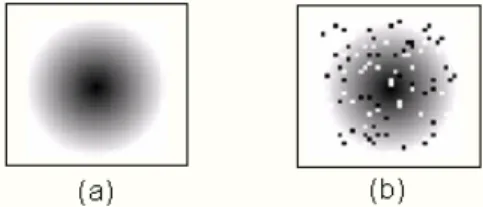
(4.3)因為我們輸入的圖片為灰階,所以這裡λ為 255,αij 表示輸入 影像在(i, j)位置的像素值,βij 表示經過處理過的影像在(i, j)位置的 像素值,m 為輸入影像的最大尺寸(這裡為 128)。其 PSNR 值為越大, 影像的品質越好,反之,則越差。以下為程式所模擬出的結果: 圖(十一) PSNR 之程式模擬圖 由圖(十一)我們可以看到整體及個別元素的 PSNR 都為無限大,這也 更能證明影像經過分離及合成過程中,並沒有遭受到破壞。 由上述可知,影像經過分離及合成過程中,並沒有遭受到破壞。 以下我們主要是利用一組給定的訓練樣本,然後搭配粒子群最佳演算 法求出細胞神經網路中類比細胞神經網路的模板“A”、“B”、“D”和 “z”。其中此組訓練樣本是由一張受到雜訊干擾的影像以及其對應的 理想未受雜訊干擾的影像所構成(也就是所訓練出的模板必定會使得
此受雜訊干擾影像經過細胞神經網路處理後會得到與其對應的理想 未受雜訊干擾的影像)。我們藉由此組給定的訓練樣本訓練出能夠消 除雜訊的模板其架構如下圖所示: 在圖(十二)中,我們主要是利用灰階的圖像作為訓練樣本(如圖(十三) 所示)並訓練出模板,用來消除其受到雜訊干擾的圖像。 (a) (b) 給定的訓練樣本 細胞神經網路 粒子群 最佳演算法 受到雜訊干擾的影像 對應理想未受雜訊干擾影像 利用粒子群最佳演算法訓練出的模板 “A”、“B”、“D”和“z” 其他受雜訊 干擾之影像 經過細胞神經網路 消除雜訊後之影像 圖(十二) 訓練架構圖
3.2 模板訓練
模板訓練
模板訓練
模板訓練
在本計劃中,我們主要是利用粒子群最佳演算法求出細胞神經網 路中類比細胞神經網路的模板“A”、“B”、“D”和“z”。其目標函數如下:(
)
∑
= − = k i d c i P i P Error 1 2 ) ( ) ( (3.1) 這裡 k 為影像的總體像素,Pc(i)為理想未受雜訊干擾影像的第 i 個像 素,Pd(i)為經過系統後雜訊消除影像的第 i 個像素。其模板訓練流程 圖及方塊圖如下圖所示: 圖(十四) 模板訓練流程圖- -- -
+
Error Pd(i) Pc(i) PSO CNN N(n) 圖(十五) 模板訓練方塊圖Part V:
:
:總結
:
總結
總結
總結
4.1 系統應用
系統應用
系統應用
系統應用
根據系統架構及訓練架構(見圖(九)、圖(十二)),我們可以針對
受到胡椒鹽雜訊(Salt and Pepper Noise)干擾的圖片,進行以下的各種 實驗。一般胡椒鹽雜訊為我們系統上常見的雜訊,也可以稱為熱雜 訊。其通常在影像上,黑點為胡椒(Pepper),白點為鹽(Salt): 實驗一 實驗一 實驗一 實驗一:::: 考慮兩張分別受到 5% 與 10%雜訊(胡椒鹽雜訊)干擾的 128 by 128 方陣之灰階影像(見圖(十六)),且利用 PSO 和 CNN 進行影像訓練 與雜訊消除,以下是我們所提出的模板以及我們所給定的 PSO 參數: 1 2 1 2 1 2 1 1 1 2 1 2 1 1 1 1 2 1 1 2 1 2 1 2 1 1 1 , , , a a a b b b d d d A a a a B b b b D d d d Z z a a a b b b d d d = = = = (4.1) 表(4.1) PSO 參數設定
The number of swarm size 10
The maximum position Xmax 1
The maximum velocity Vmax 10
Acceleration coefficient c1 1.4
Acceleration coefficient c2 1.2
Inertia weight w 0.8
(a) (b) (c) 圖(十六) (a) 未受雜訊的原始灰階影像 (b) 受 5%雜訊的灰階影像 (c) 受 10%雜訊的灰階影像 經過我們所提出的方法(PSO-CNN)可以得到以下的結果:
圖(十七) PSO-CNN 模板訓練之世代數圖 5%雜訊消除之模板參數: 0.5739 0 0.5739 0.1958 0.0256 0.1958 0 0.5739 0 , 0.0256 0.0256 0.0256 , 0.5739 0 0.5739 0.1958 0.0256 0.1958 0.6348 0.6348 0.6348 0.6348 0.5235 0.6348 , 0.2683 0.6348 0.6348 0.6348 A B D Z = = = =
10%雜訊消除之模板參數: 0.1693 0 0.1693 0.5636 0.6322 0.5636 0 0.1693 0 , 0.6322 0.6322 0.6322 , 0.1693 0 0.1693 0.5636 0.6322 0.5636 0.9627 0.9627 0.9627 0.9627 0.2697 0.9627 , 0.1016 0.9627 0.9627 0.9627 A B D Z = = = = (a) (b) 圖(十八) (a) 雜訊消除後的灰階影像(5%) (b) 雜訊消除後的灰階影像(10%) 從圖(十六)、圖(十七)和圖(十八)可以看到所提出的細胞神經網路 結合粒子群最佳演算法對於影像雜訊消除效果是良好的。但這樣還是 不足以證明它的準確性,所以我們下面將使用一套較客觀的判斷準則 -峰值信號雜訊比(Peak Signal to Noise Ratio, PSNR):
dB MSE log 10 PSNR 2 10
λ
= (4.2)∑∑
− = m m 2 ) ( 1 MSEα
β
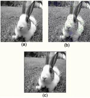
因為我們輸入的圖片為灰階,所以這裡λ為 255,αij 表示輸入 影像在(i, j)位置的像素值,βij 表示經過處理過的影像在(i, j)位置的 像素值,m 為輸入影像的最大尺寸(這裡為 128)。其 PSNR 值為越大, 影像的品質越好,反之,則越差。 用上述的方法,來驗證 PSO-CNN 的準確性,我們可以得到以下 的結果: 表(4.2) 灰階影像之峰值信號雜訊比值 受 5%雜訊干擾 受 10%雜訊干擾 原始輸入影像 16.1064dB 14.0872dB PSO-CNN 處理後影像處理後影像處理後影像 處理後影像 29.0902dB 26.8858dB 由表(4.2)以及上述所提到圖(十六)、圖(十七)和圖(十八)可以更能 充分的證明我們所提出的方法(PSO-CNN)對於灰階影像雜訊消除是 有效的。 實驗二 實驗二 實驗二 實驗二:::: 由實驗一的結果可以知道我們所提出的方法(PSO-CNN)對於灰 階影像雜訊消除是有效的,所以在這裡我們考慮兩張分別受到 5% 及 10% 雜訊(胡椒鹽雜訊)干擾的 128 by 128 方陣之彩色影像(見圖(十 九)),其模板為式(4.1)所示而 PSO 参數為表(4.1)所示,都跟實驗一所 設的參數完全一樣,以下是我們經過 PSO-CNN 所得到的結果:
(a) (b) (c) 圖(十九) (a) 未受雜訊的原始彩色影像 (b) 受 5%雜訊的彩色影像 (c) 受 10%雜訊的彩色影像
(a) (b) 圖(二十) (a) 雜訊消除後的彩色影像(5%) (b) 雜訊消除後的彩色影像(10%) 表(4.3) 彩色影像之峰值信號雜訊比值(5%) 紅 綠 藍 受5%雜訊干擾彩色影像 17.8718 dB 18.2376 dB 18.4899 dB PSO-CNN 30.2636 dB 30.3692 dB 30.1896 dB 表(4.4) 彩色影像之峰值信號雜訊比值(10%) 紅 綠 藍 受10%雜訊干擾彩色影像 14.7321 dB 15.1974 dB 15.5846 dB PSO-CNN 28.1826 dB 28.4543 dB 28.0863 dB 由圖(十九)、圖(二十)、表(4.3)、表(4.4)以及上述的實驗一結果可 以證明我們所提出的方法(PSO-CNN)對於彩色影像雜訊消除是有效 的。
4.2 結論
結論
結論
結論
我們學習到影像雜訊消除應用在細胞神經網路系統中,基於粒子 群最佳演算法,提出一個新的方法設計影像雜訊消除模板以及模板參 數更新。在不需要事先設定細胞神經網路控制模板參數的情況下,它 會設計輸入模板參數並且得到最佳的模板參數,將之用來消除受到雜 訊污染的灰階影像。與一般傳統方法設計的簡單模板大不相同,我們 提出的方法可以配合不同模板得到最佳的模板參數。舉出的例子也可 以發現我們使用的方法在恢復原始圖片上有良好的品質與效率。4.3 參考
參考
參考
參考文獻
文獻
文獻
文獻
[1] L. O. Chua and L. Yang, “Cellular neural networks: Theory”, IEEE
Trans. Circuits Syst., vol. 35, pp.1257-1272, Oct. 1988.
[2] L. O. Chua and L. Yang, “Cellular neural networks: applications”,
IEEE Trans. Circuits Syst., vol. 35, pp.1273-1290, Oct. 1988.
[3] K. R. Crounse and L. O. Chua, “Methods for image processing and pattern formation in Cellular Neural Networks: a tutorial”, IEEE
Trans. Circuits Syst., vol. 42, pp.583-601, Oct. 1995.
[4] P. Arena, L. Fortuna, G. Manganaro and S. Spina, “CNN image processing for the automatic classification of oranges”, Proc. IEEE
Int. Workshop on cellular neural networks and their applications, pp. 463-467, Dec. 1994.
[5] E. Lueder, and N. Fruehauf, “Optical signal processing for CNN's”,
Proc. IEEE Int. Workshop on cellular neural networks and their applications, pp. 45-54, Oct. 1992.
[6] P.R. Bakic, B.D. Reljin, N.S. Vujovic, D.P. Brazakovic, and P.D. Kostic, “Multilayer transient-mode CNN for solving optimization problems”, Proc. IEEE Int. Workshop on cellular neural networks
and their applications, pp. 25-30, June 1996.
[7] A. Gacsadi and P. Szolgay, “An analogic CNN algorithm for following continuously moving objects”, Proc. IEEE Int. Workshop
on cellular neural networks and their applications, pp. 99-104, May 2000.
[8] A. Paasio, A. Dawidziuk and V. Porra, “VLSI implementation of cellular neural network universal machine”, Proc. IEEE Int.
Workshop on Electronics, Circuits, and Systems, pp. 414-416, Oct. 1996.
[9] K. Halonen, V. Porra, T. Roska and L. Chua, “Programmable analog VLSI CNN chip with local digital logic”, IEEE Trans. Circuits Syst., vol. 2, pp. 1291-1294, 1991.
[10] P. L. Venetianer, T. Roska and L. O. Chua, “Analogic CNN Algorithms for Some Image Compression, Decompression and Restoration Tasks”, IEEE transactions on circuits and systems I:
Fundamental theory and applications, vol. 42, no. 5, pp. 278-284, 1995.
[11] A. Zarandy, F. Werblin, T. Roska and L. O. Chua, “Novel Types of Analogic CNN Algorithms for Recognizing Bank-Notes”, CNNA-94
Third IEEE International Workshop on Cellular Neural Networks and their Applications, pp. 273 - 278, 8-21 Dec. 1994.
[12] A. Zarandy, A. Stoffels, T. Roska, and L. O. Chua, “Implementation of Binary and Gray-Scale Mathematical on the CNN Universal Machine”, IEEE transactions on circuits and systems I:
Fundamental theory and applications, vol. 45, no. 2, pp. 163-168, 1998.
[13] J. Kennedy, R. Eberhart, “Particle swarm optimization”, IEEE
International Conference on Neural Networks, vol. 4, pp.1942-1948, 27 Nov-1 Dec 1995.
[14] X. Shenheng, R. S. Yahya , “Boundary conditions in particle swarm optimization revisited”, IEEE Transactions on Antennas and
Propagation, vol. 55, NO. 3, pp.760-765, March 2007.
[15] Y. Shi, R. Eberhart, “A Modified Particle Swarm Optimizater”,
Proceedings of the IEEE Conference on Evolutionary Computation, pp.69-73, 4-9 May 1998.
出 席出出出 席席 國席 國國 際國 際際 學際 學學 術學 術 研術術 研研 討研 討討 會討 會會 報會 報報 告報 告告告
蘇蘇蘇蘇 德德德德 仁仁仁仁
會議名稱:2009 International Conference on New Trends in Information and
Service Science 北京 NISS 研討會
會議日期:2009 年 6 月 30 日 至 7 日 2 日 會議地點:中國北京市友誼賓館
發表論文:Cellular Neural Network for Noise Cancellation of Gray Image Based on Hybrid Linear Matrix Inequality and Particle Swarm Optimization 論文編號:R1S03-256063
論文作者:Te-Jen Su(蘇德仁), Yu-Jen Lin, Chia-Ling Hou 論文頁數:pp.613---617 論文摘要如下: NISS 2009 研討會所發表的內容有關於使用線性矩陣不等式理論與粒子 群體最佳演算法探討細胞神經網路系統。其研究主題包括輸入與回授模板最 佳化的參數設計、系統穩定問題,討論細胞神經網路在灰階影像雜訊消除上 的應用。基於線性矩陣不等式理論探討系統穩定性,以粒子群最佳演算法求 得在穩定條件下模板的最佳參數,將之用來消除受到雜訊污染的灰階影像。 此次研討會共有七個議題: (1)網路安全網路安全網路安全、網路安全、、、完整性完整性完整性、完整性、、、隱私與信任議題隱私與信任議題隱私與信任議題 隱私與信任議題 探討網際網路領域中在 Web 安全性裡使用的人工智慧技術、Web 用戶和 Web 代理人的信任和談判、Web 的隱私保存、在 Web 應用過程中的隱私 保存等最新的技術。
(2)城市經營管理的方法學城市經營管理的方法學城市經營管理的方法學議題城市經營管理的方法學議題議題議題
提出不同的計算法則,應用於都市的經營管理鑑定,評價和結合的管理決 策過程中進行改進與分析。 (3)關於知識管理關於知識管理關於知識管理,關於知識管理,,,知識服務和知識的轉移知識服務和知識的轉移知識服務和知識的轉移議題知識服務和知識的轉移議題議題 議題 此議題有關於知識發現和數據采集、以知識為基礎的系統、知識服務、知 識管理和商業情報、知識轉移、決策支持系統、訊息資源共享、知識管理 和Web語義、個性化訊息服務、數字化的圖書館。 (4)在無所不在的電子服務與在無所不在的電子服務與在無所不在的電子服務與在無所不在的電子服務與商業流程開發商業流程開發商業流程開發議題商業流程開發議題議題 議題 如何透過最新技術與方法有效應用於企業界管理,並提升服務品質,在此 針對在電子服務和商業過程之間的會集技術、無線服務應用(例如:RFID, WiMax) 、無所不在的計算技術與電子服務。 (5)網路與通訊議題網路與通訊議題網路與通訊議題網路與通訊議題 針對網際網路和Web應用、測量和性能分析、多媒體聯網、網路體系架構、 網路操作和管理、基于網路的應用、聯網系統應用程式和服務、下一代網 際網路、光網路和系統、對等和覆蓋網路、QoS和資源管理、近期趨勢和 在計算機網內的發展、通訊的信號處理、無線通信、無線多媒體系統等進 行探討。 (6)金融數據采集議題金融數據采集議題金融數據采集議題金融數據采集議題 探討怎樣使用那些新近發展理論數據采集與金融數據采集。研究內容有:在 當今的金融危機方面的數據采集、在FDM裡監督學習模型/方法、時序數據 分析、在FDM裡的神經網路,決策樹和支持向量機、基於數據采集的預報 模型的股票價格、基於數據采集的預報模型的金融風險、基於數據采集的 金融欺詐察覺模型、金融隱私保護數據采集等研究內容。
(7)語意語意語意P2P網路議題語意 網路議題網路議題 網路議題 探討服務發現和使用基於語義的點對點網路、語義的點對點存儲系統、語 義的對等工作流程管理體制、語義的計算的點對點網路、基於語義的點對 點網路計算的資源搜尋機制和探索法,滿足對更多的對語義的點對點網路 的理論和應用性的研究的需要。 心得 心得 心得 心得 透過國際研討會的請益交流,了解國際學術研究最新發展,有助於日後研究 方向之新思維。近年大陸地區對於網路系統研究方面發展迅速,因此,此次 考察特別著重於網路管理系統等議題,期盼能提供授課學生們更多的新知與 研究新方向。
Cellular Neural Network for Noise Cancellation of Gray Image Based on Hybrid
Linear Matrix Inequality and Particle Swarm Optimization
Te-Jen Su
Department of Electronic Engineering National Kaohsiung University of
Applied Sciences Kaohsiung 807, Taiwan, R.O.C.
e-mail: [email protected]
Yu-Jen Lin
Department of Electronic Engineering National Kaohsiung University of
Applied Sciences Kaohsiung 807, Taiwan, R.O.C. e-mail: [email protected]
Chia-Ling Hou
Department of Electronic Engineering National Kaohsiung University of
Applied Sciences Kaohsiung 807, Taiwan, R.O.C. e-mail: [email protected]
Abstract—In this paper, the technique of noise cancellation for
gray image is presented by employing linear matrix inequality (LMI) and particle swarm optimization (PSO) based on cellular neural networks (CNN). A criterion for global asymptotic stability of CNN is presented based on the Lyapunov stability theorem, and the problem of image noise cancellation can be characterized in terms of LMIs. Based on stability conditions of LMI, the parameter of templates are obtained via PSO. The examples are given to illustrate the effectiveness of the proposed method.
Keywords- cellular neural networks, particle swarm optimization, linear matrix inequality, noise cancellation, image
I. INTRODUCTION
Cellular neural networks have been introduced by L.O. Chua and L. Yang [1, 2] in 1988. The most important key point of investigating CNN is how to find the accurate templates. In recent years, the problems of CNN templates design for image processing have received considerable attention. Genetic algorithm and multilayer CNN were presented to obtain templates for image processing in [3].
A CNN with a particular hysteresis nonlinear cell characteristic was employed for image processing in [5]. In practice, a drawback of CNN templates design is that the templates must be simplified to decrease the time of operation [3] or to analyze dynamical behavior in mathematics easily [4, 5,6].
Recently, there have been several literatures proposed to deal with the stability of CNN by choosing various Lyapunov functions [7-10]. The LMI can now be solved efficiently by the
Particle Swarm Optimization was first presented by the James Kennedy and Russell Eberhart in 1995 [12], inspired by social behavior of bird flocking or fish schooling, it has proven both very effective and quick for a diverse set of
optimization problems.
In this paper, The overall objective of this paper provides a criterion for stability of CNN based on the Lyapunov stability theorem. The problem of gray image noise cancellation can be
characterized in terms of LMIs, and the
optimization parameters of templates are obtained via PSO.
II. PARTICLESWARMOPTIMIZATION(PSO)
In PSO, suppose that the search space is D-dimensional, and then the i-th particle is represented as Xi=(xi1,xi2,K,xiD).
The velocity (rate of the position change) of this
particle is denoted as Vi=(vi1,vi2,K,viD). The best
previous position of the i-th particle is
represented as Pi =(pi1,pi2,K,piD). In other words,
Pi involves the best previous position which has visited (the local best position called pbest). The index of the best particle among all the particles in the swarm is defined as the symbol (the global best position called gbest). The particles are manipulated according to the following equations: In its canonical form,
follows: 1 1 2 2 ( 1) ( ) () ( ) () ( ) id id id id gd id v t w v t c rand p x c rand p x + = ∗ + ∗ ∗ − + ∗ ∗ − (1) ) 1 ( ) ( ) 1 (t+ =x t +v t+ xid id id (2) where ) (t 1
vid + : velocity of particle i at iteration t+1
) (t vid : velocity of particle i at iteration t ) (t 1
xid + : position of particle i at iteration t+1
) (t
xid : position of particle i at iteration t
1
c : acceleration coefficient related to pbest
2
c : acceleration coefficient related to gbest
1
rand() : random number uniform distribution
U(0,1)
2
rand() : random number uniform distribution
U(0,1)
id
P : pbest position of particle i
gd
P : gbest position of particle i
w : inertia weight
III. SYSTEMDESCRIPTION
The associated CNN state equation :
( ) ( ) ( ) ( ) ( )
(
)
( ) ( ) ( )(
)
( ) ( ) ( )(
)
( ) ( ) ( ) ( ) ( ) ( ) ( ) ( ) ( ) , , , 1 , 0 , , , , , , 1 , , , , , 0 , , , A ˆ ˆ A A ˆ B B ˆ B I r r r r r r ij ij ij kl kl C k l S i j ij kl kl ij kl kl C k l S i j C k l S i j ij kl kl ij kl kl C k l S i j C k l S i j ij kl kl ij C k l S i j x t x t y x t y x t y x t u t u t u t ∈ ∈ ∈ ∈ ∈ ∈ = − + + + + + + +∑
∑
∑
∑
∑
∑
& (3)( )
(
x t)
f(
x( )
t)
yi i = iwhere x( )t =[x1( )t ,...,xn( )t]T∈R is the state vector,
0 1,Aˆ
Aˆ
A, are the feedback matrices, B,Bˆ1,Bˆ0
are the input matrices, [ ]T
n 1,...,u u u= is the input vector, [ ]T ,..., n 1 I I I = , and ( ) (x t) 0.5
(
x( )t 1-x( )t-1)
yi i = i + i ∈[-1 +1].We assume A=Aˆ1+Aˆ0 and B=Bˆ1+Bˆ0, the
dynamical behavior of a space-invariant continuous time CNN can be described by following equations: ( ) ( ) ( ) ( ) ( ) ( ) ( ) ( ) ( ) ( ) ( ) ( ) ( ) ( ) ( ) ( ) , , , , , , , , , , , , A A B B I r r r r ij ij ij kl kl ij kl kl C k l S i j C k l S i j ij kl kl ij kl kl ij C k l S i j C k l S i j x t x t y x t y x t u t u t ∈ ∈ ∈ ∈ = − + + + + + ∑ ∑ ∑ ∑ & (4)
( )
(
x t)
f(
x( )
t)
yi i = iIn order to simplify the proof of the stability of
CNN, we will shift the equilibrium point x of *
system to the origin.
Let * x -x(t) z(t) = , (z(t)) y(x(t))-y(x*) = Φ , system (4) can be represented as
(z(t)) A (z(t)) A -z(t) (t) z& = + Φ + Φ (5) where [ ]T n 1()...z () z ) z(⋅ = ⋅ ⋅ , Φ(z(t))=[φ1(z1(t)),..., ( )T ] (t) zn n φ
Step 1: In order to prove the global asymptotic stability of the origin of (4), we choose the following positive definite Lyapunov functional:
( ) ( )
t z t 2 ( )( )
sds z V(z(t)) n 1 i t z 0 T i∑∫
= Φ + = α (6)Where α is a positive constant.
The time derivative of V(z(t)) along the
trajectories of (5) is obtained as ( ) ( ) ( ) ( ) ( ( )) ( ) ( ( )) ( ) ( ) ( ) ( ) ( ( )) ( ) ( ( )) ( ) ( ) ( ) ( ( )) ( ( )) ( ) ( ) ( ( )) ( ) ( ) ( ) ( ( )) ( ) ( ( )) ( ) ( ) ( ) ( ( )) ( ( )) ( ) (z t )A (z( )t ) 2 t z A t z 2 t z t z 2 t z A t 2z t z A t 2z t z t 2z t z A t z 2 t z A t z 2 t z t z 2 t z A t z t z A t z t z t z t z A t z t z A t z t z t z -t z V T T T T T T T T T T T T T T T T T Φ Φ + Φ Φ + Φ + Φ + = Φ Φ + Φ Φ + Φ + Φ + Φ + Φ + = α α α α α α & (7) According to T(z( )t) ( )zt T(z( )t) (z( )t) Φ Φ ≥ Φ , we can write ( ) ( ) ( ) ( ) ( ) ( ( )) ( ) ( ( )) ( ) ( ) ( ( )) ( ( )) ( ( )) ( ) (zt)A (z( )t ) 2 t z A t z 2 t z t z 2 t z A t 2z t z A t 2z t z t -2z t z V T T T T T T Φ Φ + Φ Φ + Φ Φ + Φ + ≤ α α α & (8) ( ) ( ) [ ( ) ( ( ))] ( ) ( ) ( ) ( ) ( ) ( ) Φ + + + Φ ≤ t z t z I -A A 2 A A A A 2I -t z t z t z V T T T α & (9) From (9), if
(
)
(
A A)
2(
A A-I)
0 A A 2I -T < + + + α (10)Then the time derivative of V(z( )t )is also negative
definite.
Using the Schur Complement Lemma, the inequality (10) holds if and only if
(
)
(
A A) (
A A)
0 2 1 I -A A 2α + + + T + < (11)We assumeA+A=M. Aand A are symmetric
matrices, (11) can be rewritten as
(
)
M M 0 2 1 I -M 2α + T < (12)The α is a positive constant, so (12) can be simplified 0 I -A A+ < (13)
In the above, we have demonstrated that (13) is the criterion of the global asymptotic stability of
Step 2: The uniqueness of the equilibrium point 0
=
∗
z is proved by contradiction method. Consider the equilibrium equation of (5)
( )
z -A( )
z 0 A -z - * Φ * Φ * = (14) where ∗z is the equilibrium point. From (14), it is clearly that if Φ( )z* =0, then z∗=0. Let
( )z* ≠0
Φ , multiplying both sides of (13) by (z∗) Φ , we obtain
( )
z z( ) ( )
z A z( ) ( )
z A z 0 - T * * T * * T * * = Φ Φ + Φ Φ + Φ (15) According to T(z( )t) ( )zt T(z( )t ) (z( )t ) Φ Φ ≥ Φ , equation(15) can be expressed as the following inequality
( )
z*[
A A-I]
( )
z* 0 T ≥ Φ + Φ (16)So, we can obtain
0 I -A A+ ≥ (17)
Consider the criterion for the global asymptotic stability of CNN (13), it implies that
0 I -A A+ < (18)
because equation (17) contradicts with equation (18), the equilibrium point z* =0 of (5) is
unique.
So far, the criterion of uniqueness and global asymptotic stability of the equilibrium point of CNN has been derived above. In other words, the template “A” is obtained already according to (13). Now, we will design template “B” of CNN to achieve desirable output at steady state. The dynamical behavior of CNN in (4), the equilibrium equation of (4) is show as
( )
( )
* * * 1 1 1 1 0 A A B B n n i ij j j ij j j j j n n ij j ij j j j x y x y x u u = = = = = − + + + +∑
∑
∑
∑
(19)By using the property of saturation nonlinearity, (19) is rewritten as the following inequalities
1 y 1 u u y y 1 y x u u y y 1 y 1 u u y y i n 1 j n 1 j j ij j ij n 1 j j ij n 1 j j ij i n 1 j n 1 j j ij j ij n 1 j j ij n 1 j j ij i n 1 j n 1 j j ij j ij n 1 j j ij n 1 j j ij if , b b a a 1 -if , b b a a if , b b a a i = < + + + < < = + + + = > + + + ∗ = = = ∗ = ∗ ∗ = = = ∗ = ∗ ∗ = = = ∗ = ∗
∑
∑
∑
∑
∑
∑
∑
∑
∑
∑
∑
∑
(20)IV. LMIANDPSOBASEDONCNNTEMPLATE
Figure 1. Training system
If the following LMIs are existence, then the templates of the CNN for the image
reconstruction would be solvable.
1. A+A-I<0 2. 1 y 1 u u y y 1 y x u u y y 1 y 1 u u y y i n 1 j n 1 j j ij j ij n 1 j j ij n 1 j j ij i n 1 j n 1 j j ij j ij n 1 j j ij n 1 j j ij i n 1 j n 1 j j ij j ij n 1 j j ij n 1 j j ij if , b b a a 1 -if , b b a a if , b b a a i = < + + + < < = + + + = > + + + ∗ = = = ∗ = ∗ ∗ = = = ∗ = ∗ ∗ = = = ∗ = ∗
∑
∑
∑
∑
∑
∑
∑
∑
∑
∑
∑
∑
i=1,2,3,…,MNIn this paper, we use row-wise packing scheme to describe the dynamical behavior of cell, training samples with size 32 by 32, and the sphere of influence of the radius r=1.
V. EXAMPLE
We present an example polluted by 10% of noise density interference and using CNN with LMI and PSO approach for image noise cancellation.
and its corresponding desired image.
Figure 2. Training sample (a) desired image (b) corrupted image with 10% noise
TABLE I. PSO PARAMETER SETTINGS
The number of swarm size 15 The maximum position Xmax 1 The maximum velocity Vmax 10 Acceleration coefficient c1 1.4 Acceleration coefficient c2 1.2
Inertia weight w 0.8
Iterations 300
We obtain the templates A10%, A 10%, A 10%ˆ1 ˆ0
Example: We consider the 128*128 images in Figure.3 (a) and Figure.4 (a) which were also noise images and polluted by the salt and pepper 10% noise in Figure.3 (b) and Figure.4 (b) The results of using LMI and PSO based on CNN method in Figure.3 (c) and Figure.4 (c).
Figure 3. The results of using LMI and PSO based on CNN method (10% noise).
Figure 4. The results of using LMI and PSO based on CNN method (10% noise).
Figure 5. Iterations of LMI-PSO-CNN Training
In order to calculate the performance of the presented method under different levels of noise ratio, we introduce the Peak Signal to Noise Ratio (PSNR) as
(
)
2 m 1 i m 1 j ij ij 2 y y m 1 MSE∑∑
= = − = ~ ˆ (21) dB MSE 255 10 PSNR 2 10 log = (22)where y~ij is the pixel of the ideal image, yˆij is
the pixel of the reconstruction image at the output of CNN.
TABLE II. PSNR OF LMI AND PSO-CNN FOR 10%NOISE Figure.3 Figure.4 Salt and Pepper 12.1253dB 11.5312dB LMI and PSO-CNN 32.8353dB 31.1027dB
VI. CONCLUSION
In this paper, a solution to the templates design of CNN for noise cancellation of gray image is proposed. It is shown that the design problem can
be transformed into LMIs, and the optimization parameters of templates are obtained via PSO. Hence, we have presented an effective algorithm to the templates design for gray-scale image reconstruction using LMI and PSO based on CNN.
In the future, the problem of robust templates design should be considered under the uncertain CNN systems.
REFERENCES
[1] L. O. Chua and L. Yang, “Cellular neural networks: theory”, IEEE Trans. on Circuits and Systems, Oct. 1988, 35, pp. 1257-1272. [2] L. O. Chua and L. Yang, “Cellular neural networks: applications”,
IEEE Trans. on Circuits and Systems, Oct. 1988, 35, pp.1273-1290. [3] P. D. Lopez, L. Vilarino, D. and Cabello, “Design of multilayer
discrete time cellular neural networks for image processing tasks based on genetic algorithms” , IEEE International Symposium on Circuits and Systems, May 2000, 4, pp. 133-136.
[4] L. Ming and L. Min, “The robustness design of templates of CNN for detecting inner corners of objects in gray-scale images”, IEEE International Conference on Communications, Circuits and Systems, June 2004, 2, pp. 1090-1093..
[5] R. P. Matei, “Image processing using hysteretic cellular neural networks”, IEEE International Symposium on Circuits and Systems, May 2000, 4, pp. 129-132.
[6] L. O. Chua and T. Roska, Cellular neural networks and visual computing, New York: Cambridge University Press, 2002.. [7] X. Liang, W. Tan, Z. Wan and D. Yang, “A novel criterion for glob
al asymptotic stability of cellular neural networks with time delays”, Intelligent Control and Automation, 2008 WCICA 2008,7th World Congress on, June 2008, pp. 4430-4433.
[8] Y. He, M. Wu and J.H. She, “An improved global asymptotic stability criterion for delayed cellular neural networks”, Neural Networks, IEEE Transactions on, Jan. 2006, 17, pp. 250-252. [9] V. Singh, “Global asymptotic stability of cellular neural networks
with unequal delays: LMI approach”, Electronics Letters, April 2004, 40, pp. 548-549.
[10] H. Zhang and Z. Wang “Global Asymptotic Stability of Delayed Cellular Neural Networks”, Neural Networks, IEEE Transactions on, May 2007, 18 , pp.947-950.
[11] P. Gahinet, A. Nemirovskii, A. Laub and M. Chilali, LMI Control
Toolbox: For Use With MATLAB, The MATH Works Inc., 1995. [12] J. Kennedy and R. Eberhart, “Particle swarm optimization” , IEEE