I
NTERNATIONAL
R
EAL
E
STATE
R
EVIEW
2002 Vol. 5 No. 1: pp. 133 - 145
Housing Demand with Random Group
Effects
Wen-chieh Wu
Assistant Professor, Department of Public Finance, National Chengchi University, Taiwan, or jackwu@nccu.edu.tw
Sue-Jing Lin
Associate Professor, Department of International Trade, Lunghwa University of Science and Technology, Taiwan, or sjlin@mail.lhu.edu.tw
This paper examines the random group effect, which has usually not been considered in traditional housing demand studies. Frequently, group level variables are used in housing demand estimation due to the data constraint. For instance, the US Index of Housing Price per administrative area is often used to measure the housing price when estimating the US price elasticity of demand for housing, and the average household income is often used as a proxy for the individual income in Taiwan when estimating the income elasticity of demand for housing. Econometricians argue that the traditional OLS estimation, when the random group effect is ignored, has been considered to have a downward bias in the estimated standard error. By following Amemiya (1978) and Borjas and Sueyoshi (1994), we propose a two-stage estimation technique to estimate housing demand with the random group effect. Using Taiwan’s cross-sectional survey data, we found that the standard error of the estimated coefficient for the group level income variable is underestimated in the traditional unadjusted OLS specification. This finding suggests that there may be a danger of spurious regression in the traditional OLS housing demand estimation.
Keywords
Introduction
Regression models with random group effects1 have become increasingly
popular in applied economic research. However, whether the traditional Ordinary Least Squares (OLS) technique is appropriate for estimating the linear specification with a random group effect has been questioned. For example, Moulton (1986) demonstrated that the common practice of ignoring intragroup error correlation and using OLS can lead to serious mistakes in statistical inference owing to the downward bias in standard errors. Borjas and Sueyoshi (1994) extended the existing analysis of the linear regression model to nonlinear probit specification with structural group effects. They suggested that the traditional nonlinear specification, which ignores group effects, has a considerable danger of spurious regression.
Random group effects have not yet been well applied in traditional housing demand studies, although they are indeed important there. The main reason for this is that housing demand studies must often use the group level data of explanatory variables - such as the housing price variable and the household income variable - in their estimations due to the data constraint. For instance, the US Index of Housing Price per administrative area is often used to measure housing prices when estimating the US price elasticity of demand for housing (Greenlees and Zieschang, 1984). In contrast, housing demand studies in Taiwan often use the average household income of a certain administrative area as the proxy data for individual household income (Lin, 1988; Lin, 1990, 1993; Lin and Lin, 1994, 1999; Chen and Lin, 1998)2.
Therefore, the random group effect should be considered in housing demand studies.
Furthermore, traditional housing demand studies in Taiwan have ignored possible random group effects and simply used the Ordinary Least Squares for estimation. This can lead to serious mistakes in statistical inference. Therefore, the main purpose of this paper is to examine whether the unadjusted OLS standard errors have a downward bias in housing demand studies in Taiwan.
1Regression errors are often correlated within groups because the data of the explanatory
variables in a regression model is randomly drawn from a population with a grouped structure.
2 The Annual Housing Status Survey from DGBAS does not provide information regarding
Following Amemiya (1978) and Borjas and Sueyoshi (1994)3 , we propose
an alternative two-stage approach to estimate the housing demand model with random group effects. In the first stage, we account for group (administrative area) effects by including dummy variables to allow for administrative area-specific intercepts. We then fit the estimated administrative area-specific intercepts to the average household income of the administrative area, employing GLS techniques to correct for nonspherical errors.
Using Taiwan’s cross-sectional survey data, we examine the estimated coefficients and standard errors, comparing the traditional OLS specification and the proposed two-stage estimation technique. We find that the estimated coefficients are similar in both the traditional OLS specification and our proposed two-stage estimation technique. In addition, the estimated standard errors for the price variable are close to each other in the two techniques. The estimated unadjusted OLS standard error of the income variable, however, has a downward bias, suggesting that the statistical significance of the income effect may be overstated in the traditional OLS estimation.
We organized our analysis of the importance of random group effects in housing demand studies as follows. In Section 2, we introduce the linear regression model with random group effects. In particular, the theory suggests that the unadjusted OLS specification has a downward bias in the standard error if the random group effect is taken into account in the model. Section 3 describes the econometric model and specifications we use for the estimation. Empirical analysis, including data and empirical results, is summarized in Section 4. Section 5 presents concluding remarks.
The Linear Regression Model with Random Group Effects
Moulton (1986) suggested that the random group effect has been ignored in past linear regression models. He argued that the common practice of ignoring intragroup error correlation and using OLS can lead to serious mistakes in statistical inference due to the downward bias in standard errors. We first briefly describe his arguments.
Consider a linear regression:
3 All three developed a two-stage estimator. In the first stage, they accounted for common
effects by including dummy variables to allow for group-effect intercepts. They then fitted the estimated group-specific intercepts to group level variables, using GLS techniques to correct for nonspherical errors.
ij ij
ij X v
y =
β
+ , (1)where yij is the dependent variable, is a vector of regressors, and is the error for unit i in group j. In the above, xij is a vector of explanatory variables with individual data, zj is a vector of explanatory variables common to members of group j, while vij is the independent and identical distributed errors. The group sizes are denoted by n1, … , ng where g is the number of groups.
Assume that the errors are equicorrelated within groups and the error variance, 2, is unknown. Traditionally, OLS coefficient estimators and the unadjusted (misspecified) covariance matrix, with group effects ignored, are computed using the following formula:
y X X X' ) 1 ' ( ˆ= − β , (2) ). /( ) ˆ ( , ) ( ) ˆ ( s2 X'X 1 s2 y' y X n k Var∧ β = − = − β − , (3)
However, the true covariance matrix for the OLS coefficient estimator should be given by:
1 ' ' 1 ' 2( ) ( ) ) ˆ ( = X X − XVX X X − Var β σ , (4) } ) 1 {( ' 2 i n i n i n e e I diag V =σ −ρ +ρ , (5)
where V is the disturbance covariance matrix, ρ = corr (vij , vik), j ≠ k, and
i n
e is an ni vector of ones.
The unadjusted OLS covariance matrix is different from the true covariance matrix. That is, Var∧ (βˆ)<Var(βˆ). The unadjusted OLS standard errors, therefore, have downward biases.
The Econometric Model and Specification for Housing
Demand
Traditionally, the demand for housing for individual j in metropolitan area i is specified as a function of both income and housing price4:
4We assume that there are only two goods for consumers. One is housing (H) and the other is a
ij ij ij
ij ice Income v
e
Expenditur = + logPr + log +
log β0 β1 β2 , (6)
where β2 is the income elasticity and β11 is the price elasticity of housing demand. Here, vij are independently and identically distributed errors for individual j in metropolitan area i.
If individual data had been used for all explanatory and dependent variables, there would be no need to take into consideration the random group effect. Due to the data constraint, individual data is used for expenditures (Expenditureij) and prices (Priceij), but metropolitan area average incomes (Incomei) are used for individual income variables (Incomeij) in traditional Taiwanese housing demand studies. In this case, errors should be correlated within groups (metropolitan areas), and the random group effect should be considered in the estimation. Using OLS specification and ignoring the random group effect can lead to serious mistakes in statistical inference due to the downward bias in standard errors. Therefore, we will propose a new estimation technique for the housing demand specification with random group effect.
Following Amemiya (1978) and Borjas and Sueyoshi (1994), we propose the two-stage estimation specification described as follows:
First stage: logExpenditureij=β0+β1logPriceij+di+µij , (7)
Second stage: dˆi = logγ Incomei+ωi , (8)
where β11 is the price elasticity of housing demand, is the income elasticity of housing demand, and di is the dummy variable for the administrative area i. ij are independently and identically distributed errors for individual j in metropolitan area i.
In the first stage, we use OLS to regress the log of expenditure (log Expenditureij) on both log of price (log Priceij) and the dummy for the administrative area (di). We then fit the estimated area intercepts into the log of income (log Incomei) from the second stage, employing GLS to correct for nonspherical errors.
is a log-linear functional form, log H = β0 + β1 log PH + β2 log Y + β3 log PX, where β1 + β2 + β3 = 0 because the assumptions of housing demand are homogeneous of degree zero and bear no money illusion. Therefore, we can rewrite the housing demand to housing expenditure, log(PH H / PX)= β0 + (β1 1) log(PH / PX) + β2 log (Y / PX) to get equation (6).
Empirical Analysis
Data, Sample, and VariablesThere are two data sources, the “Annual Housing Status Survey” and “Survey of Family Income and Expenditure,” both of which are conducted by the Taiwan Directorate-General of Budget, Accounting and Statistics (DGBAS).
The Annual Housing Status Survey was conducted only from 1979 to 1989, and again in 1993 due to budget constraints. The survey data was not panel data. We re-sorted the data set by the purchase year of the housing from 1971 to 1993 instead of the investigated year. Instead of using the pooling method, we choose only 1979 and 1989 cross-sectional data as the study samples. The survey data of 1979 has the largest sample sizes, while the 1993 survey year is the most recent available data5.
In this paper, we use housing expenditure as the proxy variable of housing demand because it is difficult to observe the housing service directly. There are two major explanatory variables used in the estimation: housing price and household income. Definitions of the variables in this study are summarized as follows:
Expenditure (housing expenditure): rents are the main expenditure for households. Therefore, total housing expenditure is the imputed rent for owners and the actual rent for renters.
Price (price of housing units): we used the “Annual Housing Status Survey” data set to compute the housing price per square meter along with the method proposed by Lin and Lin (1995)6. The housing price per unit is the
actual purchase price for owners and the imputed housing price for renters. Income (household yearly income): since we could not find information regarding individual household incomes, we used the Distribution of Family Income by Areas in Taiwan Area (or as we call it, the area average household income) as the income variable. This data was obtained from the “Survey of Family Income and Expenditure”. Data for Chiayi City and
5 We could obtain the data set by purchasing it for the years 1990 to 1993, but the sample size would be too small. Hence, we finally used the data from 1989.
6 The estimation method is described in the appendix of Lin and Lin (1995). They tended to use the hedonic method to estimate the housing price.
Hsinchu City was missing, so we ignored them and included only 21 administrative areas (Counties and Cities) in the sample7.
Table 1 shows the basic statistics of the data. The sample sizes were 10,052 in 1979 and 2,775 in 1989, respectively. The average rent per year was NT$18,913 in 1979 and NT$59,249 in 1989. The mean household income was NT$191,627 in 1979 and NT$485,521 in 1989. The mean housing price per square meter was NT$15,190 in 1979, and NT$17,884 in 1989. During the past decade in Taiwan, housing expenditure and average household income increased 3.13 and 2.53 times, respectively, and the growth rates were 213% and 153%, respectively.
Table 1: Basic Statistics Unit: NT$
1979 1989
Expenditure (Rents) (per year) 18,913.39 (10,615.29)
59,248.76 (38,145.10)
Average Household Income 191,626.66
(30,516.44)
485,521.48 (73,693.22)
Housing Price (per m2) 15,189.77
(24,169.91) (11,476.01) 17,884.25
Number of Observations 10,052 2,775
Data sources: “Annual Housing Status Survey” and “Survey of Family Income and Expenditure” conducted by the Directorate-General of Budget, Accounting and Statistics (DGBAS), Taiwan.
Note: Standard errors are included in parentheses.
Estimation Results
Obtained by the traditional OLS method, the estimation results of Equation (1) are shown in Table 2. All of the estimated coefficients are significant. This suggests that the price elasticity of housing demand were –0.9308 in 1979 and –0.7080 in 1989, and the income elasticity of housing demand were 0.9723 in 1979 and 1.2610 in 1989. These results show that housing is a normal good and follows the law of demand. Moreover, the character of housing tends to be a luxury after 1989.
However, the purpose of this paper is to test the random group effect, so we apply the stage method. The first-stage estimation results in the two-stage technique, as shown in Table 3. Penghu County is the base and the remaining 20 administrative areas are dummy variables.
7 Owing to the fact that the administrative area of Chiayi City and Hsinchu City was not divided in 1979, we ignored them and compared the other 21 cities with the data set in 1989.
Table 2: Unadjusted OLS Estimation Results Log Expenditure 1979 1989 Intercept -2.7288** (0.3522) -8.4927** (0.7696) Log Price 0.0692** (0.0054) 0.2920** (0.0207) Log Income 0.9723** (0.0296) 1.2610** (0.0623) Adj. R2 0.1291 0.2474 F-value 745.739** 456.89** No. of Observations 10,051 2,774
Notes: (1) Standard errors are in parentheses.
(2) ** indicates that the coefficient is statistically significant at the 5% significance level.
In Table 3, most of the coefficients are significant, and the price elasticities of housing demand are –0.9615 in 1979 and –0.7363 in 1989. Comparing the results obtained by OLS, we find that there is only a slight difference in estimated price elasticity of the same year between techniques. However, the estimated price elasticity of housing demand in Taiwan varies across different years. In 1979, the price elasticity was approximately close to –1.0, while it was around –0.70 in 1989. These estimated figures fall in the range that past studies have found in Taiwan.8
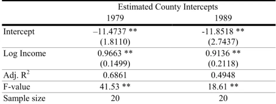
Table 2 indicates that the income elasticity of housing demand estimated by the traditional OLS was 0.9723 in 1979 and 1.2610 in 1989, respectively. As shown in Table 4, the second-stage estimation results in the two-stage technique suggest that the income elasticity of housing demand was 0.9663 in 1979 and 0.9136 in 1989, respectively. These two techniques suggest similar income elasticity of housing demand, ranging from 0.90 to 1.26. These estimated numbers also fall into the wide range that past studies have found in Taiwan.9
8. The estimated price elasticity of housing demand in Taiwan ranges from –0.17 to –1.28. See de Leeuw (1971), Lee and Kong (1977), Mayo (1981), and Lin and Lin (1994).
9. The estimated income elasticity of housing demand ranges from 0.08 to 2.05. See de Leeuw (1971), Lee and Kong (1977), Carlinear (1981), Mayo (1981), Wu 1981, 1994), and Lin and Lin (1994).
Table 3: First Stage Estimation Results in a Two-Stage Technique Log Expenditure 1979 1989 Intercept 9.0704 ** (0.0717) 8.1199 ** (0.2010) Log Price 0.0385 ** (0.0055) 0.2637 ** (0.0204) Taipei County 0.3536 ** (0.0528) 0.2709 ** (0.0506) Ilan County 0.1553 ** (0.0583) -0.4864 ** (0.0821) Taoyuan County 0.1983 ** (0.0544) 0.0292 (0.0611) Hsinchu County 0.2512 ** (0.0617) 0.0566 (0.0874) Miaoli County 0.2789 ** (0.0594) -0.2509 ** (0.0874) Taichung County 0.2264 ** (0.0553) 0.0895 ** (0.0610) Changhwa County 0.2136 ** (0.0552) 0.0333 (0.0706) Nantou County 0.1957 ** (0.0589) -0.2364 ** (0.0899) Yunlin County 0.0773 (0.0581) -0.0349 (0.0833) Chiayi County - 0.0408 (0.0604) -0.0809 (0.0891) Tainan County 0.1263 ** (0.0564) -0.1704 ** (0.0677) Kaohsiung County 0.1472 ** (0.0553) -0.0884 ** (0.0623) Pintung County - 0.0158 (0.0572) -0.2082 ** (0.0716) Taitung County - 0.1666 ** (0.0618) -0.3236 ** (0.1247) Hualien County 0.0425 (0.0604) 0.0209 (0.0815) Keelung City 0.3173 ** (0.0575) -0.0528 (0.0713) Taichung City 0.3653 ** (0.0572) 0.2689 ** (0.0581) Tainan City 0.3258 ** (0.0570) 0.1680 ** (0.0634) Taipei City 0.6716 ** (0.0529) 0.5139 ** (0.0506) Kaohsiung City 0.3679 ** (0.0538) 0.0627 (0.0547) Adj. R2 0.1740 0.2929 F-value 101.796 ** 55.72** No. of observations 10,051 2,774
Notes: (1) Standard errors are in parentheses.
(2) ** and * indicate that the coefficient is statistically significant under the 5% and 10% significance levels respectively.
Table 4: Second Stage Estimation Results in a Two-Stage Technique
with GLS (Var( ) 2*(LogIncome)2
i σ
ε = )
Estimated County Intercepts
1979 1989 Intercept –11.4737 ** (1.8110) -11.8518 ** (2.7437) Log Income 0.9663 ** (0.1499) 0.9136 ** (0.2118) Adj. R2 0.6861 0.4948 F-value 41.53 ** 18.61 ** Sample size 20 20
These two techniques obtain similar estimated coefficients of independent variables, but are quite different in the estimated standard errors. We summarize these estimated coefficients and standard errors in Table 5. The standard errors of estimated price coefficients are quite similar among techniques.
Table 5: OLS Estimator/Two-Stage Estimator
1979 1989 OLS (1) Two-stage (2) Ratio (2)/(1) OLS (1) Two-stage (2) Ratio (2)/(1) Price Elasticity -0.9308 -0.9615 1.0330 -0.7080 -0.7363 1.0400 Standard Errors (Price) 0.0054 0.0055 1.0185 0.0207 0.0204 0.9855 Income Elasticity 0.9723 0.9663 0.9938 1.2610 0.9136 0.7247 Standard Errors (Income) 0.0296 0.1499 5.0642 0.0623 0.2118 3.3997
However, the estimated standard errors of income coefficients obtained by these two estimation techniques are quite different. The traditional OLS estimated standard error of the income coefficient for 1979 was only 0.0296, whereas it was 0.1499 using the two-stage technique. The ratio of standard error estimated by the two-stage technique to the standard error estimated by the traditional OLS is about 5.0642. A similar bias in the standard error is also found in the 1989 data, where the estimated standard error from the
two-stage technique is about 3.3997 times that of the one in the traditional OLS estimation.
These findings suggest that the use of traditional OLS estimation on the housing demand study may have a downward bias in standard errors of income coefficients. This bias can be attributed to the ignorance of group effects in the traditional OLS estimation. In other words, the traditional OLS estimation may overestimate the t-ratio of coefficient of the income variable and overstate the statistical significance of the income effect. The findings of our study match both intuition and theory. As mentioned earlier, individual data is often used for housing price and expenditures, and group data is used for income variables in housing demand studies on Taiwan. In theory, the downward bias in standard error caused by the random group effect happens only with the income variable, and there should not be a bias problem on the price variable. Our empirical studies support the prediction that the downward bias problem affects the income variable but not the price variable.
Conclusion
The linear regression model with random group effect has become increasingly important in applied research. However, econometric studies suggest that traditional OLS specification is not appropriate for estimating the linear regression model with the random group effect. The major drawback of the OLS specification is the downward bias in the standard errors.
There has been little attention paid to traditional housing demand studies. Owing to the data constraint, housing demand studies often have to use the group level data of explanatory variables - such as the housing price variable and the household income variable - in their estimations. In order to consider the random group effect in housing demand estimation, this paper proposes a two-stage technique for estimating housing demand. Using both 1979 and 1989 Taiwan cross-sectional survey data, we find that both the estimated price elasticity and income elasticity in the two-stage technique are similar to those obtained by traditional OLS estimation. The estimated numbers in our study fall in the range estimated from past studies. The estimated standard errors of the price variable are similar among techniques, which agree with intuition. The price variable used in our study is the individual data. It does not have the problem of group effect.
However, the estimated standard errors of income coefficient in the traditional OLS specification are much lower than in the two-stage technique. This finding suggests that the traditional OLS specification often used in Taiwanese housing demand studies may have a downward bias in the standard error of the income variable. This is consistent with the findings of previous econometric studies indicating that the unadjusted OLS standard errors have substantial downward biases. In other words, the statistical significance of the income effect may have been overstated in past housing demand studies on Taiwan. These findings suggest that researchers should be careful when using the traditional OLS technique for estimating housing demand if the group-level variable is to be used in the study.
References
Amemiya, T. (1978), A Note on a Random Coefficients Model,
International Economic Review, 19, 793-796.
Borjas, G. and G. Sueyoshi (1994), A Two-Stage Estimator for Probit Models with Structural Group Effects, Journal of Econometrics, 64, 165-182. Carlinear, G. (1981), Income Elasticity of Housing Demand, Review of
Economics and Statistics, 55, 528-530.
Chen, C. L. and C. C. Lin (1998), Wealth Effect, Income Effect, and Housing Demand, Journal of Housing Studies, 7, 83-99. (in Chinese)
de Leeuw, F. (1971), The Demand for Housing: A Review of Cross-Section Evidence, Review of Economics and Statistics, 53, 1-10.
Greenlees, J. and K. Zieschang (1984), Grouping Tests for Misspecification: An Application to Housing Demand, Journal of Business and Economics
Statistics, 2, 159-169.
Lee, T. H., and C. M. Kong (1977), Elasticities of Housing Demand, Journal
of Southern Economics, 44, 298-305.
Lin, C. C. (1990), A Reversed Nested Multinomial Logit Model of Housing Demand and Tenure Choice, Academic Economic Papers, 18, 137-158. (in Chinese)
Lin, C. C. (1993), The Relationship between Rents and Prices of Owner-Occupied Housing in Taiwan, Journal of Real Estate Finance and
Lin, C. C. and S. J. Lin (1994), An Estimation of Price Elasticity and Income Elasticity of Housing Demand in Taiwan, Journal of Housing Studies, 2, 25-48. (in Chinese)
Lin, C. C. and S. J. Lin (1995), The Bubbles of the Housing Price in Taiwan, Taiwan Economic Association Annual Conference Proceedings, 295-313. (in Chinese)
Lin, C. C. and S. J. Lin (1999), An Estimation of Elasticities of Consumption Demand and Investment Demand for Owner-Occupied Housing in Taiwan: A Two-Period Model, International Real Estate Review, 2, 1, 110-125.
Lin, M. H. (1988), The Study of Rental Housing Demand in Taipei, Master Thesis, National Chengchi University. (in Chinese)
Mayo, S. K. (1981), Theory and Estimation in the Economics of Housing Demand, Journal of Urban Economics, 10, 95-116.
Moulton, B. R. (1986), Random Group Effects and the Precision of Regression Estimates, Journal of Econometrics, 32, 385-397.
Wu, S. T. (1981), The Income Elasticity of Housing Demand: The Empirical Results in Taipei City, Economic Studies, 23, 11-16. (in Chinese)
Wu, S. T. (1994), Income, Money and House Prices: An Observation of the Taipei Area for the Past Two Decades, Journal of Housing Studies, 2, 49-65. (in Chinese)