國
立
交
通
大
學
電子工程學系 電子研究所
碩 士 論 文
動態考慮多關鍵性迴路之效能感知佈局研究
Throughput-Aware Floorplanning by Dynamically
Considering Multiple Critical Cycles
研 究 生: 王莉雅
指導教授: 黃俊達 博士
動態考慮多關鍵性迴路之效能感知佈局研究
Throughput-Aware Floorplanning by Dynamically
Considering Multiple Critical Cycles
研 究 生:王莉雅 Student:Liya Wang
指導教授:黃俊達 博士 Advisor:Dr. Juinn-Dar Huang
國 立 交 通 大 學
電子工程學系 電子研究所
碩 士 論 文
A Thesis
Submitted to Department of Electronics Engineering & Institute of Electronics College of Electrical and Computer Engineering
National Chiao Tung University in partial Fulfillment of the Requirements
for the Degree of Master of Science
in
Electronics Engineering August 2007
Hsinchu, Taiwan, Republic of China
動態考慮多關鍵性迴路之效能感知佈局研究
研究生:王 莉 雅
指導教授:黃 俊 達 博士
國 立 交 通 大 學
電 子 工 程 學 系 電 子 研 究 所 碩 士 班
摘 要
隨著製程的進步,導線延遲取代了元件的延遲,逐漸主宰著系統的效率,並且在設 計上成為一個非常關鍵的因素。然而,導線的延遲很難在早期的系統設計中預知,必須 要等到佈局(floorplan)完成才可以有初步的分析。因此,在這份論文中,我們會介紹導 線延遲所造成的潛在因素是如何引響系統的效能,並且重新評估一些具有同成果品質 (Quality of Result) 目 標 的 舊 有 佈 局 方 法 。 接 著 我 們 提 出 一 個 新 的 效 能 感 知 (Throughput-Aware)佈局方法,這個新的方法會動態考量一個對效能最具關鍵的迴路集 合,此迴路集合的元素還會隨著佈局的過程而改變,以達到增進系統效能(system throughput)的目標。實驗結果也顯示出我們的方法可大幅增進系統效能,有些例子裡甚 至可以比以往的方法達到兩倍以上的成長。我們另外推薦一個整體設計流程,可以在系 統設計步驟時就預估佈局對效能的影響,避免未來因為效能不足而造成冗長且高價的重 複設計代價。Throughput-Aware Floorplanning by Dynamically
Considering Multiple Critical Cycles
Student: Liya Wang
Advisor: Dr. Juinn-Dar Huang
Department of Electronics Engineering
Institute of Electronics
National Chiao Tung University
ABSTRACT
The wire delay is gradually dominating the system performance and becoming one of the most critical design issues. However, it is hard to precisely estimate the wire delay in early design stages until floorplan is actually done. In this thesis, we first show how the latency incurred by wire delay dominates system throughput and re-evaluate several exiting floorplanning strategies which are considered providing the same quality of result (QoR) in the past. Then we propose a new throughput-aware floorplanning strategy which dynamically optimizes a set of most critical performance cycles in the system. The experimental results show that our approach can even double the system performance than the previous method in certain cases. We also recommend a design flow that considers the floorplanning impact as early as the system-level design stage to avoid lengthy and costly redesign iterations.
Acknowledgment
從進入研究所到這份論文的完成,我得到非常多的人的幫助以及關懷。在此我將對 他們表達我的感謝之意,如果沒有這些幫助,這份論文是無法完成的。 首先是要感謝的是我親愛的父母。他們辛苦的工作並養育我,給我一個幸福完整的 家庭,從小讓我接受良好的教育,提供我經濟的來源,讓我衣食無缺。在我研究的過程 中全力支持我、關心我,讓我無後顧之憂的完成我的研究。深厚的親情是無法用言語訴 說,在此也僅能獻上我微不足道的感謝:謝謝你們讓我順利完成研究。 重要的是我也非常感謝我的指導老師─黃俊達教授。他不僅提供了完整的研究環 境,並且花費了很多心力在我身上。如果沒有 Adar 老師的教導、解惑、以及每次的討 論,我的研究工作將會無比艱辛。再次感謝我的指導老師 Adar 老師。另外要感謝的是 Adar、Acar、以及 EDA group 的所有老師和同學們。當我上台報告 的時候,像是周景揚老師、陳宏明老師、趙家佐老師…等等,這些老師們總是會給我最 好的建議,幫助我的研究,非常感謝這些老師的幫助。而其他同學:同屆的小形和小朋 友總是會跟我一起討論課業,也會幫忙我修改報告內容;詠翔學長總是會幫我解決設備 或是工作站的問題;而在論文即將完成的後期時間,耿維學長更是給我非常大的幫助, 使我受益匪淺;另外還有其他學長姐學弟妹的關心討論等等。很多的幫忙,像是同學之 間的加油打氣、研究苦思時的體貼關懷,都無法一一寫出,我只能在此表達我的感謝之 意,謝謝這些人的關懷以及幫助,也讓我的研究生活充實而愉快。 對於此論文的完成,我有很多的感激。一份論文的研究實在需要很多很多的助力, 不論是實際上的支持,或是背後的幫助,皆無法在此以三言兩語來真正的說明,因此在 最後引用陳之藩先生說的話:「因為需要感謝的人太多了,就感謝天吧。」來表達我完 成論文的心情,謝謝。
Contents
1 Introduction……….. 1
1.1 Motivation………... 4
1.2 Our Contribution……… 5
1.3 Organization of This Thesis………... 5
2 Preliminaries………... 6
2.1 System Throughput……… 6
2.2 The Effect of Floorplanning to Throughput……….. 10
2.3 Problem Formulation………. 11
2.4 Related Works……… 12
2.4.1 The Modified SA-based Adjacent Constraint Graph (ACG) Floorplaner[14]……… 12
2.4.2 The SA-based Floorplaner with Correlative Cost Function[9]………… 14
3 Throughput-Aware Floorplanning by Dynamically Considering Multiple Critical Cycles ………. 16
3.1 The Consideration of Multiple Critical Cycles……… 16
3.2 Dynamic Cycle Set CTp……… 18
3.3 The SA-based Flow of Our Approach……….. 20
4 Experimental Results………. 22
4.1 Environment Setup and Benchmarks……… 22
4.2 Weight Assignment……… 23 4.3 Results……… 23 4.3.1 Experiment I……… 23 4.3.2 Experiment II……….. 25 4.4 Stability……….. 26 4.5 Discussion……….. 28
5 Throughput-Aware Design Flow………. 29
6 Conclusion……….. 32
Reference……… 33
List of Figures
1-1 Un-shrinking global wire as feature size downscaling………..……… 1
1-2 The trend for signal propagation length (obtained from [2])………... 2
1-3 An example of the pipeline element insertion……… 3
2-1 The system nFB without feedback loop………... 6
2-2 Time slot sequence in the system nFB……… 7
2-3 The system FB with feedback loop………. 8
2-4 Time slot sequence in the system FB………... 8
2-5 The system with two cycles………. 9
2-6 Time slot sequence of the system in Figure 2-5……….. 10
2-7 Floorplanning results FP1 & FP2……… 10
2-8 Floorplan FP1 & FP2 after pipelining………. 11
2-9 The system S1 and its floorplanning result FS1-a………. 13
2-10 The floorplanning result FS1-b of the system S1……….. 13
3-1 The cycle means of 10 cycles in a system……….. 16
3-2 The possible cycle means at the beginning (a) and ending (b) in SA process……... 18
3-3 The flow chart of SA-based floorplaner……….. 21
4-1 Average throughput improvement for Method_M, Method_C, and Method_D….. 25
4-2 Average throughput improvement of Method_D and Method_D*……… 26
4-3 The standard deviations for every method under different number of cycles……… 27
5-1 The redesign iterations……….. 29
List of Tables
3-1 The meanings of the abbreviations in Figure 3-3……….. 20 4-1 The number of blocks and cycles for every benchmark………. 22 4-2 Average throughput and dead space……….. 24 4-3 Average area overhead for Method_M, Method_C, and Method_D………….…… 25 4-4 Average area overhead for Method_D and Method_D*………. 26 A-1 Average P and DS of every bnechmark………35
Chapter 1
Introduction
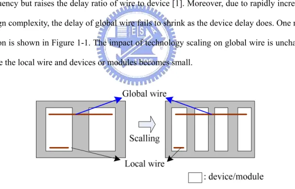
As entering the era of SoC design using deep submicron (DSM) technology, the trend of continuous shrinking device size and interconnect width makes the performance critically dependent on the latency of long wires. Feature size downscaling speeds up the operating frequency but raises the delay ratio of wire to device [1]. Moreover, due to rapidly increasing design complexity, the delay of global wire fails to shrink as the device delay does. One major reason is shown in Figure 1-1. The impact of technology scaling on global wire is unchanged while the local wire and devices or modules becomes small.
Figure 1-1. Un-shrinking global wire as feature size downscaling.
As a result, the length which a signal can reach within a clock cycle drops quickly. Figure 1-2, which is obtained from [2], shows the trend for metric clock locality in different process generation. The die length is 30mm and the operating frequency is 1.2GHz. In the
can reach within a clock cycle decreases to only 5% of the die length in the 60nm process node. 0.25 0.18 0.13 0.1 0.08 0.06 1 2 4 8 16 0 10 20 30 40 50 60 70 80 90 100
processor generation (um)
clocks Die reachable (%)
Figure 1-2. The trend for signal propagation length (obtained from [2]).
Hence, it is unavoidable that the chip-scale inter-module communication becomes multi-cycle. Such multi-cycle latency can seriously degrade the performance improvement originally obtained from adopting advanced fabrication technology. The combination of increasing long wire delay and increasing chip operating frequency forces designers to innovate better design methodologies.
Therefore, in physical level, there are wire sizing, buffer insertion, bus encoding…etc helping to relax the wire delay constraint. And in system level, many research works try to find new design paradigms that not only have advantage of being perfectly transparent to the designers but still guarantee the timing closure and correct functional behavior.
One approach is to adopt globally-asynchronous locally-synchronous (GALS) systems [3-5] which utilize asynchronous handshake protocols for global inter-module communication.
The other is to use latency-insensitive systems (LIS) [6-8] in which the communication protocols do not rely on specific latency requirements. In such protocol, modules are surrounded by wrappers and communicate through special pipeline elements, called relay stations. Another one is network-on-chip (NoC) platform [9-10] which organizes the global wire as an on-chip interconnection network. The communication of NoC design passes through every module’s router with network interface.
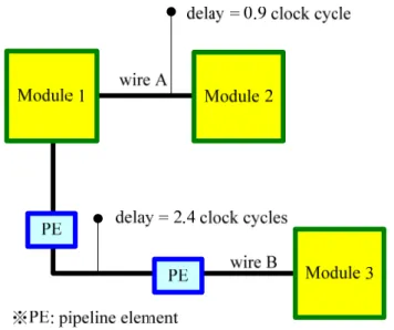
For synchronous designs, inserting pipeline elements into interconnects, like LIS design paradigm and wire pipelining strategy, is generally compatible with the traditional synchronous design mainstream. The LIS design is getting more attention these years and wire pipelining is used popularly. By inserting pipeline elements into interconnects, the time constraint is relaxed. For example, the wires shown in Figure 1-3, the input/output time constraint of wire for all the modules are needed to be smaller than 1 clock cycles. The delay of wire A is 0.9 clock cycle such that it needs no pipelining. On the other side the delay of wire B is 2.4 clock cycles such that two pipeline elements are inserted into wire B. Therefore, the input/output timing constraint of wire B is feasible.
1.1 Motivation
For synchronous design, how to realize multi-cycle communication is addressed well. However, besides the overhead of additional pipeline elements, it also jeopardizes overall system throughput due to the existence of multi-cycle communication feedback loops within the system.* If this issue can not be properly addressed, the advantage obtained from technology improvement is likely to vanish as mentioned previously.
Moreover, notice that it is particularly hard to deal with this throughput degradation issue in early system design stage. This is because the wire delay information remains unknown until the floorplanning is actually performed. Thus, how many clock cycles for the interconnect communication is dependent on the result after performing floorplan. Therefore, the floorplan needs to be modified appropriately to deal with this important subject otherwise the system performance is endangered. The floorplaner that considers multi-cycle communication becomes necessary and is very important in the coming era of high speed synchronous design.
The overall system throughput is virtually unpredictable at early design phase. If the throughput result after floorplanning doesn’t meet the requirement, significant redesign iterations are likely required to achieve the target throughput. These redesign iterations may become a terrible encumbrance and damage the project schedule. Hence, the effect of floorplan to the throughput must be evaluated in advance. As a result, a more effective design flow is needed to minimize the redesign iterations.
1.2 Our Contribution
In this thesis, a new floorplanning strategy is proposed. This strategy is based on simulated annealing (SA) and the cost function is defined to considering the important issue of system performance—throughput. Moreover this new strategy dynamically considers a set of most critical cycles. This dynamic set of cycles is initially set to certain range of cycles according to their throughput and its size changes with temperature. It has a good balance between high correlation and low sensitivity than previous works. The experimental results show that our method provides significant improvement on throughput. Furthermore, the improvement of our method increases very much as the interconnect delay gets larger.
According to the experiment of optimizing the throughput, a global design flow is recommended. This recommended design flow evaluates the throughput result affected by floorplanning after system-level design. If the throughput result is not satisfied at this stage, it can be fast backward to change the system-level design and doesn’t need to wait until finishing the backend floorplan. Thus, this new design flow helps reduce the redesign iterations between backend floorplan backward to system-level architecture or RTL & logic design stages.
1.3 Organization of This Thesis
This thesis is organized as follows. In Chapter 2 we show the preliminaries for our work. It includes the throughput calculation, the effects of floorplanning to throughput, and the related works. The proposed throughput-aware floorplanning strategy is given in Chapter 3. Experimental results are provided in Chapter 4. The recommended overall design flow is discussed in Chapter 5. Chapter 6 concludes this thesis.
Chapter 2
Preliminaries
2.1 System Throughput
Data rate is the major performance metric in system design and it is calculated by multiplying the system throughput and the operating frequency. Obviously, the throughput serves as an important performance factor. As described, the throughput depends on not only the latency of functional blocks but also the latency incurred by long wires. An example is given to show how the wire latency impacts the throughput.
Figure 2-1. The system nFB without feedback loop.
Consider the system nFB shown in Figure 2-1, the circles a, b, and c are functional blocks, while the rectangle PE is a pipeline element. Assume the interconnect delay between
a and c is greater than one clock period but less than two. It implies that at least one pipeline
element must be inserted between a and c to preserve the correct functionality. Hence, the interconnection latency from a to c is 1 clock cycle. Assume the latency of every functional
block is 1 clock cycle. Also assume that the interconnect channel can properly queue the transfer data. The output sequence at the functional block c is considered as the output of the system nFB.
At the time slot t0, all functional blocks a, b, and c produce the first valid data tokens a0, b0, and c0 while PE only contains an empty data token τ initially. For following time slots,
every functional block produces a valid data if its input data are ready at the previous time slot. Otherwise it produces empty data. A pipeline element only keeps a token one clock cycle then forwards it out from senders to receivers.
Figure 2-2. Time slot sequence in the system nFB.
In Figure 2-2, at time slot t1, because one input data of the block c is τ at the previous
time slot, c produces τ and the data b0 is queued in the interconnecting channel from b to c.
Also at time slot t1, the pipeline element PE receives the data a0, and passes it to the block c
at the next time slot. Then the empty data τ is popped out since t2 and all functional blocks
produce valid data since then. Note that there exists only one τ in the output sequence of the system nFB. Therefore the overall throughput of the system nFB approaches 1 as t→∞.
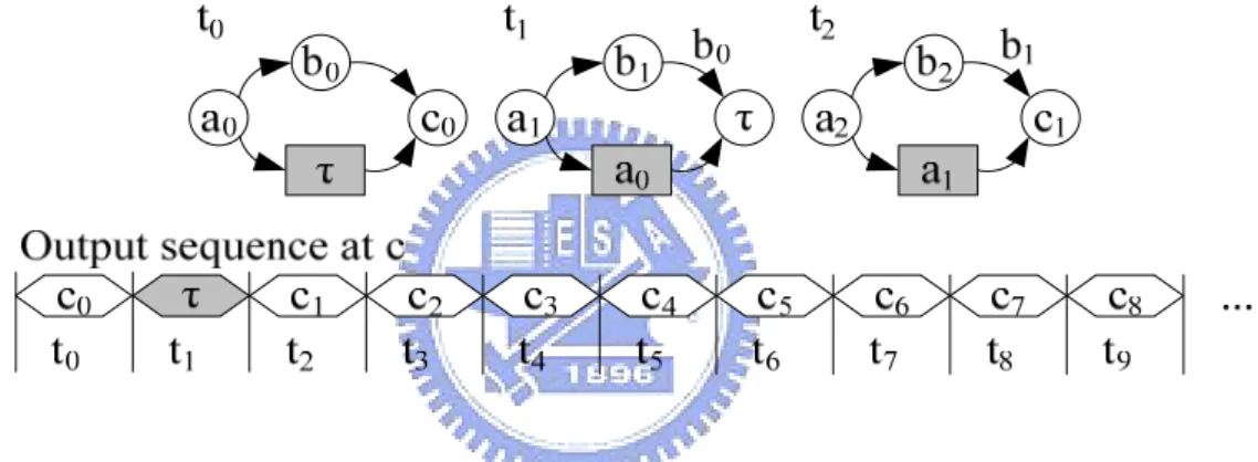
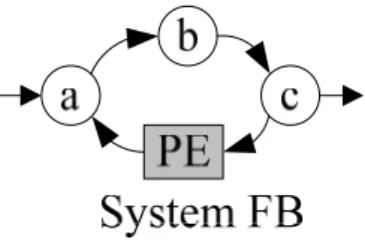
Now consider the system FB with a feedback loop as shown in Figure 2-3. Though it looks similar as the system nFB, it presents a totally different throughput.
Figure 2-3. The system FB with feedback loop.
As Figure 2-4 points out, the empty data token τ introduced by PE circles around during
t0 ~ t4. It becomes obvious that the empty data token never disappears and always presents at
the system output every 4 clock cycles. As a result, the throughput of the system FB approaches only 3/4 as t→∞.
Figure 2-4. Time slot sequence in the system FB.
As the two systems nFB and FB demonstrate, a system can be modeled as a graph, in which vertices depict the functional modules and edges describe inter-module communication channels. Every vertex and edge has a weight indicating its required number of clock cycles for signal transmission. The throughput P of a cycle C can be calculated as the reciprocal of the cycle mean λ and is shown in Equation (1)
1 1 ( ) − − ⎟⎟ ⎠ ⎞ ⎜⎜ ⎝ ⎛ = = C C W PC λC (1) In Equation (1), |C|, usually called the size of cycle C, is the number of vertices in C and
W(C) is the sum of weights of all vertices and edges within the cycle C.
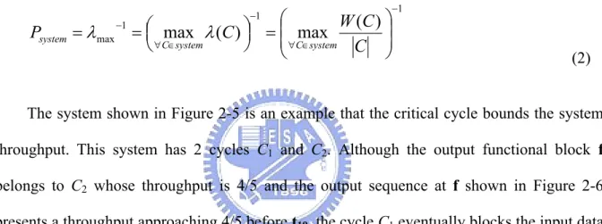
If a system contains more than one cycle, then the system throughput is bounded by the most critical cycle possessing the maximum cycle mean, shown in Equation (2). The equation has been proven in [7-8] and [16].
1 1 1 max ) ( max ) ( max − ∈ ∀ − ∈ ∀ − ⎟⎟ ⎠ ⎞ ⎜⎜ ⎝ ⎛ = ⎟ ⎠ ⎞ ⎜ ⎝ ⎛ = = C C W C P system C system C system
λ
λ
(2) The system shown in Figure 2-5 is an example that the critical cycle bounds the systemthroughput. This system has 2 cycles C1 and C2. Although the output functional block f
belongs to C2 whose throughput is 4/5 and the output sequence at f shown in Figure 2-6
presents a throughput approaching 4/5 before t19, the cycle C1 eventually blocks the input data
of the block d such that the throughput of functional block f is 3/4 after t19. Thus, the final
throughput of this system is bounded by the cycle C1 with the maximum cycle mean and
approaches 3/4 as t→∞.
4
3
1P
=
C
:
5
4
2P
=
C
:
Figure 2-6. Time slot sequence of the system in Figure 2-5.
2.2 The Effect of Floorplanning to Throughput
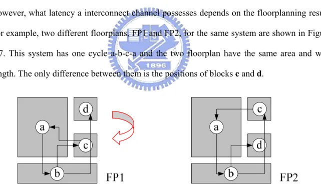
In the previous section, how wire latency affects system throughput is described. However, what latency a interconnect channel possesses depends on the floorplanning result. For example, two different floorplans, FP1 and FP2, for the same system are shown in Figure 2-7. This system has one cycle a-b-c-a and the two floorplan have the same area and wire length. The only difference between them is the positions of blocks c and d.
Figure 2-7. Floorplanning results FP1 & FP2.
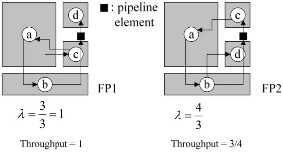
It is assumed that the data transfer cannot be successfully completed from b to d in FP1 and from b to c in FP2 within one clock cycle. Hence, a pipeline element must be inserted in both cases. After inserting pipeline elements, surprisingly, the performances of two floorplans are significantly different. As shown in Figure 2-8, FP1 remains its throughput to be 1 while
FP2’s throughput drops from 1 to 3/4 (25% performance loss).
1
3
3 =
=
λ
3 4 =λ
Figure 2-8. Floorplan FP1 & FP2 after pipelining.
This example shows the strong effect of floorplanning to throughput. If the floorplan without carefully dealing with this issue, the degradation of throughput becomes large. Therefore, we try to find a new method that improve the system throughput under simular area and wire length cost.
2.3 Problem Formulation
This problem is formulated to be a modified floorplan problem. The modifications are the input data type and the additional new objective. It can be further formulated as following.
Given: 1. A system task graph with physical information
2. The wire length that a signal can reach within one clock cycle, WCLK (The
wire length WCLK is used to calculate the latency on an interconnect.)
Constraint: A non-overlap feasible floorplan result
Objective: 1. Maximize throughput (i.e. minimize the maximum cycle mean) 2. Minimize area and wire length
In an SA-based floorplanning algorithm, the cost function is the guide to reach the objectives. Conventionally the cost function only contains the objectives for area and wire length. We add a new one for maximizing throughput into cost function Φ, and it is now defined as Equation (3).
Cost function:
Φ
=
αA
+
βW
+
γ
⋅
f
(P
)
(3)In Equation (3), A is for total area, W is for total wire length, f(P) represents the cost of throughput. Smaller f(P) means higher throughput. α, β, and γ are weighting constants. If one objective is emphazied, raising its weighting constant can make the floorplan be better on the objective.
2.4 Related Works
The floorplan with throughput consideration has been discussed. There are two related works with discussion as in the following sections.
2.4.1 The Modified SA-based Adjacent Constraint Graph (ACG)
Floorplaner[14]
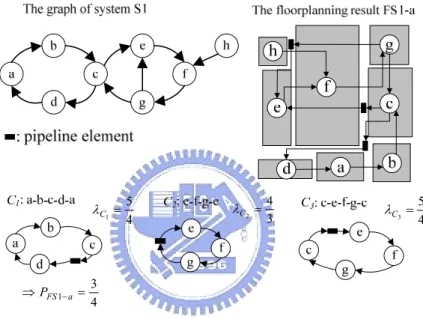
In [14], authors identify the maximum cycle mean among all cycles and directly use that mean as f(P) of the cost function in their SA-based floorplaner [15]. This method immediately gives the response of the overall system throughput in cost function without considering any minor factors. The high correlation between cost and throughput is provided. However, the maximum cycle mean might not be smooth enough to serve as a good cost function.
For example, consider the system S1 and the floorplan FS1-a shown in Figure 2-9. This system has three cycles C1, C2, and C3. According to FS1-a, the cycle C2 is the critical cycle
with the maximum cycle mean and it dominates this system throughput bounded to be 3/4. The other two cycles have equal cycle mean to be 5/4.
In order to improve the throughput, the floorplaner tends to choose a result improving the critical cycle C2. As a result shown in Figure 2-10, the cycle mean of C2 is improved from
4/3 to 1, however, the cycle mean of C3 (=3/2) takes the place of critical cycle and the system
throughput decreases from 3/4 (of FS1-a) to 2/3 (of FS1-b).
4 5 1 = C λ 3 4 2 = C λ 4 5 3 = C λ 4 3 1 = ⇒PFS −a
Figure 2-9. The system S1 and its resulting floorplan FS1-a.
1 3 3 2 = = C λ 2 3 4 6 3 = = C λ 3 2 1 = ⇒ PFS − b 1 C λ
From this example of the system S1, directly using the maximum cycle mean to be f(P) of the cost function may increase the other minor cycle means. Thus, f(P) must be considered to prevent the increasing of critical and minor cycle means simultaneously.
2.4.2 The SA-based Floorplaner with Correlative Cost
Function[11-13]
In [11-13], authors first investigate the throughput-driven floorplanning. They introduce a simulated annealing (SA)-based floorplaner optimize for system throughput. However, they claim that the throughput is too sensitive to small local changes such that it is not a good idea to directly use it in the cost function.
Instead, they create a correlative f(P) for preventing the pipeline element insertion into the edges in the critical cycles. Initially, every edge is assigned a weight with the reciprocal of the smallest cycle size containing it. It is because the pipeline element insertion in the cycle with small size is easy to decrease the system throughput. If an edge with a large reciprocal value, inserting pipeline element into the edge has much danger to the throughput. Then at each following iteration, the edge latency is updated according to the current floorplanning solution. After that, the SA-based floorplaner is guided to reduce the sum of product of the weight and the latency for all edges. The small value of this method means that the less pipeline elements in the critical edges such that the system throughput is improved. Taking the resulting floorplan of the system S1 shown in Figure 2-9 as an example, the edge g-e has one pipeline element and its smallest cycle size is |C3| =3. Hence the partial cost of it is 1/3. The
respected the partial cost of edge c-d is 1/4 and edge c-e is 1/4. Thus the final cost of f(P) of this method is 10/12.
throughput for SA-based floorplaner due to its modest sensitivity to local changes and fast computation. However, the fact is that the overall system throughput solely depends on the most critical cycle with the maximum cycle mean. Thus, it is arguable how strong the correlation between the designated cost function and the final system throughput is. According to the claim in [11], the throughput with smaller cost is better than the other one. For example, to reduce the cost of FS1-a in Figure 2-9, which is computed to be 0.83 (10/12), the FS1-b in Figure 2-10 could be the new floorplan because it has smaller cost 0.75 (9/12). However, FS1-b with throughput 0.75 (3/4) is actually better than that of FS1-a with throughput 0.67 (2/3). Therefore, neither the weighted edge cost nor the most critical cycle mean can improve the actual system throughput very well.
Chapter 3
Throughput-Aware Floorplan by
Dynamically Considering Multiple
Critical Cycles
3.1 The Consideration of Multiple Critical Cycles
According to the discussion in section 2.4, a new method for f(P) is considered in order to balance the correlation and sensitivity. Therefore, instead of the overall cycles in [11] and the maximum cycle mean in [14], a set of most critical cycles is taken into consideration in our methodology. The set of most critical cycles is defined as CTp and the number of cycles in
CTp is defined as its size |CTp|. The cycles in CTp are chosen according to their cycle means
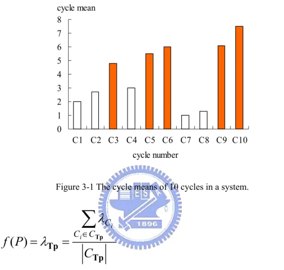
and the |CTp| is parameterizable. For example, assume we have ten cycles in a system, Figure
3-1 shows the cycle means of these cycles. The number in x-axis is the cycle number and the height of the bar is the cycle’s corresponding cycle mean.
In this example, if we decided to choose the 50% most critical cycles, then the cycles with 50% larger cycle means (C3, C4, C5, C9, and C10 which are colored in Figure 3-1) are picked up to form CTp and |CTp| is five in the floorplaner. f(P) now designed to considering
how to improve the cycle means in CTp. Minimizing the cycle mean of each cycle in CTp is
represent the influence of throughput in the cost function. Therefore, the f(P) in Equation (3) can be rewritten as Equation (4).
cycle mean 0 1 2 3 4 5 6 7 8 C1 C2 C3 C4 C5 C6 C7 C8 C9 C10 cycle number
Figure 3-1 The cycle means of 10 cycles in a system.
Tp Tp Tp
C
P
f
C C C i i∑
∈=
=
λ
λ
)
(
(4)In our work, the chosen cycles’ percentage is initially set in SA floorplaner. However, Equation (4) is not ideal application of f(P). Although this method gives the opportunity to
prevent forming a worse critical cycle from the minor ones, it has the criticism mentioned in section 2.4.2 that the small cost may not imply good throughput result. In addition, as mentioned in section 2.1, the system throughput is only decided by the maximum cycle mean. Thus it seems that keeping fixed number of multiple cycles in CTp during whole SA iterations
3.2 Dynamic Cycle Set C
TpAlthough the cycle set CTp is high correlative and not so sensitive to local change, the
computing method of λTp is still not good enough to stand for the system throughput
improving. It is always that the maximum cycle mean bounds the system throughput. Thus when SA process is near to the end, we should concentrate on decreasing the maximum cycle mean only. On the other words, CTp should eventually contain only the cycle with the
maximum cycle mean at low annealing temperature (i.e. |CTp| becomes on the end of SA
iterations). It is more practical than to consider multi-cycle for the final floorplanning result. An example is shown in Figure 3-2. (a) is represents the cycle means at the beginning iteration of floorplanning and (b) is the cycle means at almost the end of the floorplan. The cycle means in (a) are worse that needs to consider the most critical cycles. But during the SA iterations, λTp decreases such that the most cycle means are small in (b). Therefore, the
multiple cycle consideration is not suitable for (b). On the other words, reducing the maximum cycle mean is the best way under (b)’s condition.
cycle mean 0 1 2 3 4 5 6 7 C1 C2 C3 C4 C5 C6 C7 C8 C9 C10 cycle number cycle mean 0 1 2 3 4 5 6 7 C1 C2 C3 C4 C5 C6 C7 C8 C9 C10 cycle number
Figure 3-2. The possible cycle-means at the beginning (a) and ending (b) in SA process. However, dramatically drop of |CTp| should be avoided in the SA process. For SA
algorithm, it is a gradually converging process and a violent changing may destroy the process. Therefore, the violent decreasing change of |CTp| may damage the smooth characteristic of
SA-based floorplanning algorithm such that the throughput may not be improved. Thus we develop a mechanism to decrease |CTp| smoothly during SA process.
Assume that when temperature going down, the most cycle means in CTp decrease such
that the non-critical cycles increase. Therefore, |CTp| can be shrunk as temperature cooling
down and should contain only the cycle with maximum cycle mean near the end of SA iterations. T means the annealing temperature in SA algorithm and r is the cooling down ratio
of T (i.e. Tnew = rTold) and 0 < r < 1. In order to guarantee that CTp remains only the cycle with
maximum cycle mean, a threshold of temperature, called Tthreshold, is given. Therefore, |CTp|
decrease with the same down ration r of T as T greater than or equal to Tthreshold. This formulation of |CTp| is given in Equation (5).
⎪⎩
⎪
⎨
⎧
<
≥
=
threshold threshold old Tp newT
T
T
T
C
r
C
,
,
Tp1
(5)Consequently CTp is the set of most critical cycles which change according their cycle
means and |CTp| decreases with the temperature until T is smaller than Tthreshold. The initial value of CTp is decided by how worse the cycle mean is wanted to be improved. The other
parameter Tthreshold can be decided by when the multiple cycles consideration should be finished. By this dynamically considering the multiple critical cycles, λTp in Equation (4) just
3.3 The SA-based Flow of Our Approach
Combining the SA-based floorplanning algorithm with our approach, the flow chart of Figure 3-3 displays the whole process for the new throughput-aware floorplanning. The abbreviations in Figure 3-3 are described in Table 3-1. G is the system task graph with hard blocks physical information. X is the representation of a floorplan. FP( ) is the floorplanning
generation to generate a new X. p is the acceptance probability decided by the cost and
temperature. R is a random number between 0~1.
Table 3-1: The meanings of the abbreviations in Figure 3-3. G The system task graph
T Annealing temperature
r The cooling speed of Temperature X Floorplan
FP( ) Floorplanning generation
Φ Cost
p Acceptance probability R Random number
This flow is separated into three main processes that are discussed as following:
1. Initial setup: In this process, the parameters, like initial temperature, chip aspect ratio, temperature cooling down ratio…etc, are given. All cycles in the system task graph are identified and the initial set of CTp is also determined.
2. SA iteration: This is the main process of the SA-based floorplaner. At every iteration it generates a new floorplan Xnew and the new cost of this floorplan is computed. If
the cost does not change any more or T is decreased to zero, the iteration stops.
Otherwise, the judgement of taking Xnew or not is applied and the floorplaner
decreases |CTp| with temperature by Euqation (5). The cycles of CTp are also
decreasing cost or the greater computed acceptance probability than a random number. Then the next new floorplan is continuously generated.
3. Final result: It outputs the best floorplan in the SA process and it throughput.
Input data: G, T Initialize: X =X0 Φ =Φ0 1. Initial setup Terminate? Φdecreased ? Yes Xnew = FP(G, X, T) Tp λ γ βW αA+ + = Φ
,T)
p( Δ
p
=
Φ
X = X X= Xnew No No Tnew= rTold ⎪⎩ ⎪ ⎨ ⎧ < ≥ = threshold threshold T T T T C r C , , Tp Tp 1 R< p? No Yes 2. SA iterationOutput final result Yes
3. Final result
Chapter 4
Experimental Results
4.1 Environment Setup and Benchmarks
The benchmarks we use contain two sets, MCNC and GSRC. However, the original benchmarks lack of transfer direction information. In order to add data dependency between the modules in each benchmark, we break each net into a 2-pin net and randomly assign it with a direction. The system has cycles because of this direction assignment. To provide a moderate number of cycles in a system, we limit the number of cycles around one tenth the number of blocks in every benchmark. The number of cycles in every benchmark is show in Table 4-1 after our modification.
Table 4-1. The number of blocks and cycles for each benchmark
MCNC GSRC file name
apte xeorx hp ami33 ami49 n10 n30 n50 n100 blocks 9 10 11 33 49 10 30 50 100
cycles 4 2 1 5 7 2 3 9 12
The experiments are conducted on a Linux workstation with two Intel Xeon 3.2G CUPs and 3GB DRAM.
4.2 Weight Assignment
The weight of each block in a benchmark is assigned to be one. This means that each block requires one clock cycle for computation. The weight of an interconnect ei is the number of pipeline elements it needing and this number is determined by how many clock cycles a signal propagates from the interconnect’s one end to the other. For example, and interconnect with 2.4 clock cycle delay needs to be inserted into two pipeline elements. Therefore, the weight of ei is defined by Equation (6)
⎥
⎦
⎥
⎢
⎣
⎢
=
CLKW
)
length(e
)
weight(e
i i (6)The interconnect length is modelled as the Manhattan distance between the centers of two blocks. Equation (6) computes the clock cycle delay of ei and takes the floor value which is the number of pipeline elements needed at least for ei.
To model the effect of the advancing technology, we assume WCLK to shorten as 1/k times
of the die length and give several kind of k. We applied k to be the number of 1, 2, 4, …to 32.
1 means that the signal can reach the die length in one clock cycle in 0.25 um processor generation [2]. 32 is the required cycle for cross-chip signal propagation through the top-level metal wire in 35nm processor generation [18].
4.3 Results
4.3.1 Experiment I
We apply four different methods for cost computation in the same floorplaner: Method_A is like the conventional floorplaner optimizing are only. The other methods not
the maximum cycle mean only [13]; Method_C is re-implementation of the correlative cost in [10]; and Method_D is our approach. In our method, CTp initially contains all cycles and
Tthreshold is set as 1/1000 of the initial temperature.
Under the same value of k, we run every benchmark for ten times by using the four
different methods. The results of average throughput and dead space are shown in Table 4-2.
P is the system throughput and DS is the percentage of dead space.
Table 4-2. Average throughput and dead space.
Method_A Method_M Method_C Method_D
k P DS(%) P DS(%) P DS(%) P DS(%) 1 0.73 8.15 0.92 8.41 0.99 8.38 1.00 8.49 2 0.45 7.75 0.64 8.68 0.76 9.92 0.88 10.69 4 0.26 8.04 0.39 8.35 0.49 9.96 0.63 12.51 8 0.15 7.94 0.23 8.58 0.26 9.94 0.41 12.18 16 0.07 7.95 0.12 8.59 0.14 9.84 0.22 12.69 32 0.04 7.74 0.06 8.50 0.07 10.26 0.11 12.54
Form Table 4-2, the throughput decreases very much as k increases. The dead space of
our method is smaller than 13% while Method_A and Method_M are smaller than 9% and Method_C is smaller than 11%. The throughput of our method (Method_D) always has better throughput results than others.
The comparison between the four different methods on the thoughput is shown in Figure 4-1. The area overhead is shown in Table 4-3. All the results are normalized to Method_A.
Form Figure 4-1, the improvement of throughput is increasing as the number of cycles increasing and our method has the best achievements. The area overhead, which does not exceed 5%, is quite small as shown in Table 4-3.
The improvement of throughput 0% 50% 100% 150% 200% 250% 1 2 4 8 16 32 k Method_M Method_C Method_D
Figure 4-1. Average throughput improvement for Method_M, Method_C and Method_D. Table 4-3. Average area overhead for Method_M, Method_C, and Method_D
k Method_M (%) Method_C (%) Method_D (%) 1 0.24 0.21 0.31 2 0.85 2.04 2.78 4 0.30 1.81 4.19 8 0.58 1.86 3.97 16 0.59 1.77 4.43 32 0.71 2.37 4.50
4.3.2 Experiment II
In this experiment, we try to allow more are overhead by decreasing the weighting constant α in our method, called Method_D* and do the experiment of Method_D*. The
comparisons of throughput and area overhead of Method_D and Method_D* are shown in Figure 4-2 and Table 4-4. The data is also normalized to Method_A.
The improvement of throughput 0% 50% 100% 150% 200% 250% 300% 1 2 4 8 16 32 k Method_D Method_D*
Figure 4-2. Average throughput increasing of Method_D and Method_D*. Table 4-4. Average area overhead for Method_D and Method_D*
k Method_D (%) Method_D* (%) 1 0.31 1.42 2 2.78 2.76 4 4.19 7.90 8 3.97 9.36 16 4.43 10.43 32 4.50 9.79
According to Figure 4-2 and Table 4-4, if more area overhead is allowed, even more significant improvement of throughput can be achieved as the value of k increases. It shows that the area overhead increase about 10% but the improvement of Method_D* increases near to 300% as k=32.
4.4 Stability
for the results of each benchmark. The results are shown in Figure 4-3. 1 2 4 8 16 32 Method_D* Method_D Method_CMethod_M Method_A 0.00 0.50 1.00 1.50 2.00 2.50 3.00 3.50 4.00 4.50 5.00 k
The average standard deviation of the maximum cycle means
Method_D* Method_D Method_C Method_M Method_A
Figure 4-3. The standard deviations for every method under different number of cycles. From Figure 4-3, Method_A has the greatest standard deviation because it does not condiering throughput at all. Among all the throughput-aware floorplan, Method_M has the greatest standard deviation because it considers only the maximum cycle mean. And our method has smaller standard deviation than Method_C because improving the throughputs for all cycles by [10] may not actually improve the system throughput. Moreover, our method considers a set of multiple critical cycles with dynamically decreasing size, thus it really improves the system throughput at low temperature.
Method_D* has smaller standard deviation than Method_D because the more area overhead is allowed in Method_D*. Therefore, the floorplaner has more opportunities to place
4.5 Discussion
In Experiment I, the throughput degrades is very fast as the required number of cycles increases. Therefore, all method for optimizing throughput has improvement of throughput and the improvement of throughput increases when the number of cycles increases (i.e. the wire delay becomes worse). When the number of cycles is small, the improving of throughput has little difference. It is because the wire weight is still small such that achieving high throughput is easy. Our throughput-aware floorplanning shows the greatest improvement on the throughput. Even when the number of cycle increases, our approach has more improvement than other methods. It reaches almost 200% improving when the number of clocks is 16 and 32 cycles. Moreover, the area overhead of our method is no more than 5% corresponding to the Method_1.
In Experiment II, Method_4* has even more improvement than Method_4. It can have more than 250% improvement when the number of clocks is greater than 16. And the area overhead is only increasing about 9%. Thus if relaxing area constraint is allowed, the better throughput is achieved than having area constraint.
In section 4.4, our method has the smallest standard deviation between Method_1~Method_4*. Therefore our method can provide a more stable result than other methods. Specially, Method_4* which relax the area constraint has smaller standard deviation than Method_4. It may be because that relaxing area constraint makes the more possible positions for the movements of the blocks become large. Thus the standard deviation of relaxing area constraint is smaller than having it.
Chapter 5
Throughput-Aware Design Flow
Our experimental results show a great improvement can be achieved on the system throughput by using our method. However, if the result given by the throughput-aware floorplaner still can not satisfy the design constraint, redesign iteration is unavoidable. Figure 5-1 shows a design process from the system-level design to floorplanning.
Throughput-aware floorplaner RTL & logic design System-level design
Figure 5-1. The redesign iterations.
If the throughput-aware floorplaner can not generate a satisfied result, the RTL & Logic design is modified again and expects to get an improved result after performing floorplan. However, if this redesign iteration is useless on improving throughput, the system-level architecture is needed to be rebuilt. Nevertheless the throughput of the rebuilt system
architecture is still unknown until floorplan is done. Thus an un acceptable resulting throughput of the floorplan makes the design process repeat form system level to floorplan. Such redesign iterations cost too much time and decrease the benefit.
Therefore, we propose a new methodology that can help to reduce the possible design iterations. The flow of this throughput-evaluation methodology is shown in Figure 5-2. The gray part is the proposed new design stages for reducing the redesign iterations form floorplan back to system level. It helps evaluate the throughput at early design stage.
System-level design with
estimated physical information
Preliminary floorplanning
throughput evaluation
Throughput satisfied?
Througput satistied?
Futher
improvement at
RTL?
No Yes No No Yes YesRTL & logic design
Throughput-aware
floorplanning
Placement & routing
Figure 5-2 The recommended global design flow chart for preliminary throughput. First the functional blocks are give the estimated physical information of area size and the clock-latency. Then, our proposed method can be applied to calculate the preliminary throughput value for floorplanning. If the resulting throughput is not satisfied, it can
immediately modify the system-level design such that the possibility of redesigns from floorplan back to system level is greatly reduced.
Chapter 6
Conclusions
In this thesis, a new throughput-aware floorplanning strategy is proposed to maximize the system performance. It optimizes a dynamic set of most critical cycles simultaneously. Thus a more stable and better result can be obtained. Compared to the previous works, our approach is not only highly correlated to the final system throughput but also insensitive and stable to the locally minor changes during floorplanning refinement processes in floorplanning. The experimental results show that our floorplaner can achieve about twice the throughput of that minimizing area only as the applied clock cycles increasing to 16~32. And the area overhead only increases about 3%~10% more area under various setting of applied cycles. Meanwhile, a recommend design flow is proposed for preliminary throughput-aware floorplanning in system level. It helps reduce the design iterations. Hence, we believe the proposed method and flow can provide better floorplan solutions in the coming multi-cycle communication era.
Reference
[1] I International Technology Roadmap for Semiconductors, Semiconductor Industry Association, 2003.
[2] D. Matzke, “Will physical scalability sabotage performance gains?” IEEE Computer, vol.
30, pp. 37-39, 1997.
[3] D. M. Chapiro, “Globally-asynchronous locally-synchronous systems,” Ph.D. dissertation, Stanford Univ., CA, 1984.
[4] D. S. Bormann and P. Y. Cheung, “Asynchronous wrapper for heterogeneous systems,” in Proc. ICCD, pp.307-314, 1997.
[5] J. Muttersbach, T. Villiger and W. Fichtner, “Practical design of globally-asynchronous locally-synchronous systems,” in Proc. ASYNC, pp. 52-59, 2000.
[6] L. P. Carloni, K. L. McMillan, A. Saldanha and A. L. Sangiovanni-Vincentelli, “A methodology for “Correct-by-construction latency insensitive design,” in Proc. ICCAD,
pp. 309-315, 1999.
[7] L. P. Carloni and A. L. Sangiovanni-Vincentelli, “Performance analysis and optimization of latency insensitive protocols,” in Proc. DAC, pp. 21-26, 2001.
[8] R. Lu and C. Koh, “Performance optimization of latency insensitive systems through buffer queue sizing of communication channels,” in Proc. ICCAD, pp. 227, 2003.
[9] S. Kumar, A. Jantsch, J-P. Soininen, M. Forsell, M. Millberg, J. Oberg, K. Tiensyrja, and A. Hemani, “A network on chip architecture and design methodology” in Proc. Symposium on VLSI, pp. 117-124, 2002.
[10] A. Hemani, A. Jantsch, S. Kumar, A. Postula, J. Öberg, M. Millberg, and D. Lindqvist, “Network on a chip: an architecture for billion transistor era,” in Proc. of the IEEE NorChip Conf., 2002
[11] M. R. Casu and L. Macchiarulo, “Floorplanning for throughput,” in Proc. ISPD, pp.
62-69, 2004.
[12] M. R. Casu and L. Macchiarulo, “Throughput-driven floorplanning with wire pipelining,” in IEEE Tran. CAD, vol. 24, pp. 663-675, 2005.
[13] M. R. Casu and L. Macchiarulo, “Floorplan assisted data rate enhancement through wire pipelining: a real assessment,” in Proc. ISPD, pp. 121-128, 2005.
[14] J. Wang, H. Zhou and P. Wu, “Processing rate optimization by sequential system floorplanning,” in Proc. ISQED, pp. 340-345, 2006.
[15] H. Zhou and J. Wang, “ACG-adjacent constraint graph for general floorplans,” in Proc. ICCD, pp. 572-575, 2004.
[16] R. Lu and C. Koh, “Performance analysis and efficient implementation of latency insensitive systems,” ECE technical report, Purdue Univ., IN, 2003.
[17] D. F. Wong and C. L. Liu, “A new algorithm for floorplan design,” in Proc. DAC, pp.
101-107, 1986.
[18] V. Agarwal, M.S. Hrishikesh, S.W. Keckler, and D. Burger, “Clock rate vs IPC: the end of the road for conventional microarchitectures,” in Proc. ISCA, pp. 248-259, 2000.
Appendix
The average throughput and dead space of every benchmark with Method_A, Method_M, Method_C, Method_D, and Method_D* is shown in Table A-1.
Table A-1. Average P and DS of every benchmark apte
Method_A Method_M Method_C Method_D Method_D*
k P DS (%) P DS (%) P DS (%) P DS (%) P DS (%) 1 0.751 1.59 1.000 2.48 1.000 1.84 1.000 1.93 1.000 2.22 2 0.462 1.64 0.729 2.26 0.722 6.89 1.000 12.12 1.000 3.35 4 0.245 1.59 0.413 2.04 0.400 4.14 0.602 4.77 0.685 5.71 8 0.134 1.64 0.228 2.06 0.215 3.30 0.338 7.43 0.348 5.52 16 0.070 1.64 0.120 2.33 0.112 2.87 0.170 4.95 0.205 4.87 32 0.034 1.64 0.060 2.21 0.059 3.22 0.090 6.35 0.107 4.47 xeorx
Method_A Method_M Method_C Method_D Method_D*
k P DS (%) P DS (%) P DS (%) P DS (%) P DS (%) 1 0.833 6.04 0.909 6.16 1.000 6.33 1.000 6.98 1.000 6.69 2 0.435 5.85 0.541 6.31 0.909 9.64 1.000 10.29 1.000 8.89 4 0.215 5.60 0.323 6.74 0.455 10.79 0.667 22.88 0.656 19.13 8 0.122 6.09 0.174 5.73 0.242 10.87 0.351 19.39 0.388 17.48 16 0.057 5.60 0.103 6.86 0.137 10.84 0.190 22.61 0.213 18.81 32 0.033 5.70 0.047 6.50 0.069 12.40 0.097 21.23 0.110 17.51
hp
Method_A Method_M Method_C Method_D Method_D*
k P DS (%) P DS (%) P DS (%) P DS (%) P DS (%) 1 1.000 7.84 1.000 7.91 1.000 7.39 1.000 7.16 1.000 9.70 2 0.714 7.65 1.000 9.25 1.000 7.28 1.000 8.05 1.000 8.52 4 0.476 6.76 0.667 7.64 1.000 7.13 1.000 8.66 1.000 9.33 8 0.333 7.93 0.500 8.21 0.500 7.83 1.000 9.22 0.500 11.40 16 0.135 7.55 0.250 8.14 0.333 7.66 0.500 9.48 0.333 10.60 32 0.092 6.76 0.141 7.76 0.167 8.44 0.250 9.57 0.167 12.50 ami33
Method_A Method_M Method_C Method_D Method_D*
k P DS (%) P DS (%) P DS (%) P DS (%) P DS (%) 1 0.665 10.29 0.930 10.24 0.980 11.04 1.000 11.21 1.000 11.01 2 0.361 10.42 0.579 10.68 0.656 11.27 0.784 11.52 1.000 14.52 4 0.246 11.16 0.341 9.75 0.349 11.07 0.509 13.61 0.800 23.11 8 0.124 10.24 0.182 9.97 0.192 10.89 0.325 13.30 0.493 27.84 16 0.063 10.59 0.106 10.59 0.096 11.48 0.173 13.00 0.261 26.43 32 0.028 10.15 0.048 10.18 0.051 11.13 0.084 11.54 0.148 26.42 ami49
Method_A Method_M Method_C Method_D Method_D*
k P DS (%) P DS (%) P DS (%) P DS (%) P DS (%) 1 0.649 10.19 0.930 10.24 1.000 9.65 1.000 9.84 1.000 10.80 2 0.400 8.99 0.579 10.68 0.701 10.69 0.968 11.63 1.000 12.49 4 0.218 9.66 0.341 9.75 0.424 10.81 0.632 12.22 0.910 17.15 8 0.128 9.73 0.182 9.97 0.215 11.29 0.358 10.86 0.588 24.06 16 0.074 9.61 0.106 10.59 0.109 10.74 0.176 12.53 0.331 28.10 32 0.032 9.84 0.048 10.18 0.067 10.50 0.111 11.64 0.183 25.34 n10
Method_A Method_M Method_C Method_D Method_D*
k P DS (%) P DS (%) P DS (%) P DS (%) P DS (%) 1 0.728 6.48 1.000 6.02 1.000 6.82 1.000 7.16 1.000 6.06 2 0.504 5.71 0.760 6.54 1.000 9.92 1.000 8.30 1.000 8.13 4 0.255 6.28 0.471 6.90 0.656 11.73 0.752 11.26 0.752 10.44 8 0.154 6.04 0.236 6.40 0.360 10.64 0.429 10.18 0.429 10.70 16 0.074 6.09 0.126 6.35 0.203 11.59 0.271 12.76 0.267 11.97 32 0.036 5.74 0.071 6.71 0.102 11.93 0.148 12.26 0.137 12.59
n30
Method_A Method_M Method_C Method_D Method_D*
k P DS (%) P DS (%) P DS (%) P DS (%) P DS (%) 1 0.755 10.33 0.930 11.24 1.000 11.29 1.000 11.37 1.000 10.32 2 0.414 10.19 0.519 11.28 0.667 11.57 0.828 12.76 1.000 11.74 4 0.234 10.78 0.338 10.91 0.390 11.56 0.582 15.18 0.930 23.16 8 0.147 10.09 0.180 12.10 0.210 12.37 0.308 14.68 0.588 21.82 16 0.067 10.67 0.095 10.97 0.120 11.70 0.220 15.15 0.317 24.90 32 0.039 10.06 0.050 10.94 0.058 12.70 0.090 14.27 0.175 23.91 n50
Method_A Method_M Method_C Method_D Method_D*
k P DS (%) P DS (%) P DS (%) P DS (%) P DS (%) 1 0.635 9.46 0.794 9.10 0.973 10.17 1.000 9.57 1.000 12.81 2 0.385 9.22 0.583 9.17 0.596 10.87 0.693 9.78 0.976 14.67 4 0.233 9.04 0.324 9.46 0.369 10.44 0.484 11.16 0.679 22.79 8 0.117 9.59 0.179 9.85 0.190 10.52 0.277 11.04 0.405 24.05 16 0.060 9.50 0.098 9.83 0.095 10.50 0.146 10.87 0.222 22.84 32 0.032 9.00 0.047 9.98 0.049 10.54 0.080 10.72 0.117 24.43 n100
Method_A Method_M Method_C Method_D Method_D*
k P DS (%) P DS (%) P DS (%) P DS (%) P DS (%) 1 0.548 11.15 0.760 12.01 0.980 10.85 1.000 11.16 1.000 14.25 2 0.353 10.12 0.481 11.53 0.606 11.14 0.661 11.74 0.990 18.03 4 0.209 11.46 0.270 11.03 0.324 11.97 0.449 12.85 0.623 19.12 8 0.116 10.14 0.157 12.05 0.182 11.70 0.300 13.56 0.385 26.73 16 0.063 10.35 0.069 10.77 0.098 11.21 0.163 12.83 0.227 25.97 32 0.029 10.74 0.038 11.64 0.048 11.49 0.080 15.26 0.114 29.13
![Figure 1-2. The trend for signal propagation length (obtained from [2]).](https://thumb-ap.123doks.com/thumbv2/9libinfo/8262486.172246/10.892.168.755.232.746/figure-trend-signal-propagation-length-obtained.webp)