應用於多輸入多輸出通道之低複雜度多模式訊號偵測演算法與超大型積體電路實現

全文

(1)國立交通大學資訊科學與工程研究所碩士論文. 應用於多輸入多輸出通道之低複雜度多模式訊號偵測演算法與超大型積體電路實現 Low-Complexity Multi-Mode Signal Detection Algorithm and VLSI Implementation for Multiple-Input Multiple-Output Channels. 研究生：吳廸優指導教授：范倫達. 博士. 中華民國九十七年八月.

(2) 應用於多輸入多輸出通道之低複雜度多模式訊號偵測演算法與超大型積體電路實現 Low-Complexity Multi-Mode Signal Detection Algorithm and VLSI Implementation for Multiple-Input Multiple-Output Channels 研究生：吳廸優. Student：Di-You Wu. 指導教授：范倫達博士. Advisor：Dr. Lan-Da Van. 國立交通大學資訊科學與工程研究所碩士論文 A Thesis Submitted to Institute of Computer Science and Engineering College of Computer Science National Chiao Tung University in partial Fulfillment of the Requirements for the Degree of Master in Computer Science August 2008 Hsinchu, Taiwan, Republic of China. 中華民國九十七年八月.

(3) 摘要. 應用於多輸入多輸出通道之低複雜度多模式訊號偵測演算法與超大型積體電路實現. 學生：吳廸優. 指導教授：范倫達博士. 國立交通大學資訊科學與工程研究所. 摘. 要. 在本論文中，我們使用平行消除干擾、群組干擾壓縮及遞迴之技術提出一個應用於多輸入多輸出通道之廣義平行群組遞迴(GPGI)偵測框架，並提出一個低複雜度多模式演算法。所提出之偵測框架可調整三項參數與三種子演算法以達到效能與複雜度的取捨。所提出的框架平台不只包含傳統的 BODF 偵測、群組偵測、遞迴偵測與 B-Chase 偵測演算法，並且衍生出一種新的低運算複雜度且多模式之 GPGI-T1 偵測演算法。在使用 8 個傳送天線與 8 個接收天線及輸入不編碼之 16-QAM 符號下，與 BODF 偵測演算法相比，在最低複雜度的情況下，GPGI-T1 演算法能夠減少 33.9%的複雜度，並且在效能上還勝過 10 dB。在另一個情況下， GPGI-T1 演算法與 B-Chase 演算法相比，能夠降低 36.8%的複雜度而只損失 0.4 dB。最後，根據所提出之 GPGI-T1 演算法，我們使用 TSMC 0.18 um 製程實作出一多模式之多輸入多輸出訊號偵測器，可使用在傳送天線與接收天線各為二或四的情況下，支援 QPSK、16-QAM、64-QAM 之調變。並且，在五個特定應用晶片中，此實作有較好的功率效益。. I.

(4) Abstract. Low-Complexity Multi-Mode Signal Detection Algorithm and VLSI Implementation for Multiple-Input Multiple-Output Channels. Student：Di-You Wu. Advisor：Dr. Lan-Da Van. Institute of Computer Science and Engineering College of Computer Science National Chiao Tung University. ABSTRACT In this thesis, we use parallel interference cancellation (PIC), group interference suppression (GIS) and iteration techniques to construct a generalized parallel grouped-iterative (GPGI) detection framework and one new low-complexity algorithm for multiple-input multiple-output (MIMO) channels. The proposed detection framework provides three parameters and three sub-algorithms to configure a range of tradeoffs between performance and complexity. The presented framework not only covers the conventional BLAST-ordered decision feedback (BODF), grouped, iterative, and B-Chase detection algorithms, but also derives the GPGI-Type 1 (GPGI-T1) detection algorithm with low computational complexity. In (8,8) system with uncoded 16-QAM inputs, one instance of the GPGI-T1 algorithm not only substantially reduces the complexity by 33.9% but also outperforms the BLAST-ordered decision feedback algorithm by 10 dB. Another instance of the GPGI-T1 algorithm can save complexity by 36.8% at the penalty of 0.4 dB loss compared with the B-Chase detector. Last, II.

(5) Abstract. according to the proposed GPGI-T1 algorithm, we implement a multi-mode MIMO signal detector in TSMC 0.18 um CMOS process. The resulting implementation can work in (2,2) or (4,4) system, and supports QPSK, 16-QAM, and 64-QAM modulation modes. Importantly, the resulting MIMO detection implementation possesses the comparable power efficiency among five ASIC designs.. III.

(6) 誌謝. 誌. 謝. 首先感謝指導教授范倫達老師在這兩年多以來的悉心指導與建議，並提供我各方面的協助，使我可以確立並完成我的論文研究，並在我的研究過程中所提出的種種建議，讓我找到方向、抓住目標。在此先對范倫達老師致上由衷的感激。其次是 VIPLab 的夥伴們，特別感謝彥澤、旭昇學長在研究與使用 EDA 軟體上幫助，以及同窗籐耀、晉豪、宗融與得安在研究與課業上的幫忙，並感謝你們在我的研究生生活中所帶來的溫馨與歡笑。最後要感謝家人和親友們的關心、支持與鼓勵，尤其是親愛的父親吳明龍先生與母親陳季蓉女士，你們讓我可以無後顧之憂的完成學業。最後感謝女友瑋婷，謝謝妳一路陪著我從大學一直到研究所，在我低潮、壓力大的時候，始終陪在我身旁，默默忍受著我的脾氣，支持我，讓我快樂的度過這幾年，謝謝！. IV.

(7) Contents. Contents 摘. 要 ................................................................................................................. Ⅰ. ABSTRACT ........................................................................................................... Ⅱ 誌. 謝 ................................................................................................................. Ⅳ. CONTENTS ........................................................................................................... Ⅴ LIST OF TABLES ................................................................................................. Ⅶ LIST OF FIGURES .............................................................................................. Ⅷ. Chapter 1. Introduction ......................................................................................... 1. 1.1 Motivation ..................................................................................................... 2 1.2 Thesis Organization....................................................................................... 3 Chapter 2. Review of the MIMO Detection Algorithms ....................................... 4. 2.1 MIMO System Model ................................................................................... 4 2.2 Grouped Detection ........................................................................................ 5 2.3 Iterative Detection ......................................................................................... 6 2.4 Chase Detection ............................................................................................ 7 2.5 GPIC Detection ............................................................................................. 8 V.

(8) Contents. Chapter 3. Generalized Parallel Grouped-Iterative (GPGI) MIMO Detection. Framework ................................................................................................... 10 3.1 Steps of GPGI Framework .......................................................................... 12 3.2 The Properties of GPGI Framework ........................................................... 12 Chapter 4. New Type GPGI-Based Detection Algorithm ................................... 15. 4.1 Implementation of GPGI-Type1 ................................................................. 15 4.2 Reducing Complexity Highlight ................................................................. 21 Chapter 5. Complexity Analysis, Simulation Results, and Implementation ..... 23. 5.1 Complexity Analysis ................................................................................... 23 5.2 Simulation Results ...................................................................................... 26 5.3 Complexity-Performance Tradeoff ............................................................. 32 5.4 VLSI Implementation.................................................................................. 34 Chapter 6. Conclusion and Future Work ........................................................... 42. Bibliography .......................................................................................................... 44 Autobiography ....................................................................................................... 48. VI.

(9) List of Tables. List of Tables Chapter 3 2.1:. Cases of the Chase detection algorithm .......................................................... 8. Chapter 3 3.1:. Cases of the GPGI framework for MIMO detection .................................... 14. Chapter 5 5.1:. Computational complexity of the GPGI-T1 algorithm ................................. 25. 5.2:. Complexity comparison among the proposed GPGI-T1 and conventional algorithms ..................................................................................................... 25. 5.3:. Performance selection by choosing different list length ............................... 37. 5.4:. Chip characteristics of the multi-mode GPGI-T1 detector ........................... 40. 5.5:. Supplied modes of the GPGI-T1 chip implementation................................. 40. 5.6:. Comparison of ASIC implementation for MIMO detection ......................... 41. VII.

(10) List of Figures. List of Figures Chapter 2 2.1:. A MIMO system with N transmitters and M receivers ................................... 5. 2.2:. Block diagram of the grouped detection ......................................................... 6. 2.3:. An Example of the iterative detection at 4 transmitted symbols .................... 7. 2.4:. Block diagram of the Chase detection ............................................................ 8. 2.5:. Block diagram of the GPIC detection ............................................................. 9. Chapter 3 3.1:. BER performance comparison with GD and ID algorithms in (8,8) MIMO system ........................................................................................................... 11. 3.2:. Block diagram of the GPGI framework ........................................................ 11. Chapter 4 4.1:. Processing pseudo code for the implementation of the GPGI-T1 detection algorithm for Imax≧1 .................................................................................... 20. 4.2:. Processing pseudo code for the proposed modified GIS implementation .... 21. 4.3:. Processing pseudo code for the proposed DF implementation that modified from [17] ....................................................................................................... 21. VIII.

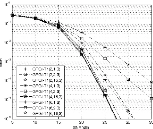
(11) List of Figures. Chapter 5 5.1:. BER performance of the GPGI-T1 algorithm with different K and  in (8,8) MIMO system with 16-QAM inputs. ........................................................... 27. 5.2:. BER performance of the GPGI-T1 algorithm with different Imax and  in (8,8) MIMO system with QPSK inputs. ....................................................... 28. 5.3:. BER performance of the GPGI-T1 algorithm and conventional algorithms in (4,4) MIMO system with QPSK inputs. ....................................................... 28. 5.4:. BER performance of the GPGI-T1 algorithm and conventional algorithms in (4,4) MIMO system with 16-QAM inputs. ................................................... 29. 5.5:. BER performance of the GPGI-T1 algorithm and conventional algorithms in (6,6) MIMO system with QPSK inputs. ....................................................... 29. 5.6:. BER performance of the GPGI-T1 algorithm and conventional algorithms in (6,6) MIMO system with 16-QAM inputs. ................................................... 30. 5.7:. BER performance of the GPGI-T1 algorithm and conventional algorithms in (8,8) MIMO system with QPSK inputs. ....................................................... 30. 5.8:. BER performance of the GPGI-T1 algorithm and conventional algorithms in (8,8) MIMO system with 16-QAM inputs. ................................................... 31. 5.9:. BER performance of the GPGI-T1 algorithm and conventional algorithms in (4,6) MIMO system with QPSK inputs. ....................................................... 31. 5.10:. BER performance of the GPGI-T1 algorithm and conventional algorithms in (4,6) MIMO system with 16-QAM inputs. ............................................ 32. 5.11:. Complexity-performance trade-off of the GPGI-T1, B-Chase and GPIC(1,0) algorithms with QPSK inputs. .................................................................... 33. IX.

(12) List of Figures. 5.12:. Complexity-performance trade-off of the GPGI-T1, B-Chase and GPIC(1,0) algorithms with 16-QAM inputs. ............................................................... 34. 5.13:. Block diagram of the GPGI-T1 algorithm .................................................. 34. 5.14:. Block diagram of the implementation of the GPGI-T1 algorithm. ............. 35. 5.15:. BER performance of the GPGI-T1 algorithm and B-Chase algorithm in (4,4) MIMO system with 64-QAM inputs. ......................................................... 37. 5.16:. Pipeline architecture of the multi-mode GPGI-T1 detector. ....................... 38. 5.17:. Chip layout of the multi-mode GPGI-T1 detector. ..................................... 39. 5.18:. Post-layout simulation of the multi-mode GPGI-T1 detector. .................... 40. X.

(13) Chapter 1 Introduction. Chapter 1 Introduction Multiple-Input-Multiple-Output (MIMO) technology can significantly improve data transmission rate in bandwidth-limited wireless communications without increasing transmission power. Much research [1-2] has shown that the channel capacity increases with the number of antennas. Because of the above benefit, the MIMO technique has been considered in modern high-speed wireless communication standard including wireless LAN [3] and mobile wireless MAN. For the MIMO communication systems, the detection scheme is more complex than that in the SISO communication systems. Since the MIMO communications transmit information at very high data rates, the low computational complexity detection algorithm at the receiver is essentially considered. In terms of detection performance, the maximum likelihood (ML) detection scheme is an optimum solution at the receiver. However, it is manifest that the detection complexity raises as the number of antennas and the constellation size increases. Therefore, the computational complexity of the ML scheme is too huge for hardware implementation and unsuitable for high-speed communications. The sphere decoding (SD) scheme [4]-[6] searching for the closest lattice point inside the radius bounded sphere achieves the same performance of the ML detection with efficient computational complexity. However, the complexity of the SD algorithm is unstable owing to the variation of the iteration number which is higher at low signal to noise ratio (SNR) 1.

(14) Chapter 1 Introduction. environment especially. Hence, the SD algorithm has higher computational complexity at low SNR communication environment due to the larger iteration numbers. On the other hand, the variable throughput of the SD algorithm also affects the system performance.. The. Bell. Laboratories. layered. space-time. (BLAST). wireless. communication system [1] uses multi-element antenna arrays at both the transmitter and receiver to achieve high spectral efficiency. This technology is referred to as the diagonal BLAST (D-BLAST). The D-BLAST theoretically approaches the Shannon capacity for multiple transmitters and receivers, but the D-BLAST is complex and impractical. The vertical BLAST (V-BLAST) system [7], [8] is a simplified architecture of the D-BLAST, where the BLAST-ordered decision feedback (BODF) detection algorithm named in [16] (also called successive interference cancellation (SIC) detection algorithm named in [19]) is applied. Although the BODF algorithm has low computational complexity, the poor bit-error rate (BER) performance is incurred. Other efficient implementations of the BODF algorithm [9], [10] aim at low-complexity computation but still possess poor BER performance.. 1.1 Motivation Many researchers currently concentrate on developing detection algorithms in both complexity and performance between the ML and BODF detection algorithms [11], [12]. The above research work divides symbols into two groups by two schemes. The QR-decomposition [11] is partially applied to the channel matrix such that two sub-channels are orthogonal to each other. The second scheme [12] uses group interference suppression (GIS) technique [13] to divide the V-BLAST system into two lower dimensional sub-systems. After group partition, the first-group symbols are detected by the ML detection and the second-group symbols are detected by a 2.

(15) Chapter 1 Introduction. suboptimal algorithm after cancelling the interference from the first-group symbols. Although the previous published schemes using the ML and suboptimal detection algorithms can achieve better performance, the high computational complexity is incurred. Thus, we are motivated to devise a MIMO detection algorithm that features the low computational complexity and satisfactory performance. Furthermore, in order to trade off the performance and complexity for different demands, we develop a framework to cover the previous and proposed algorithms.. 1.2 Thesis Organization This thesis is organized as follows. Brief review of the MIMO detection algorithms is described in Chapter 2. In Chapter 3, one generalized parallel grouped-iterative (GPGI) framework has been presented. In the same chapter, how to generate existing algorithms through this framework will be discussed. In Chapter 4, we propose one new low complexity detection algorithm via this framework. We present the complexity analysis, performance simulation and chip implementation results in Chapter 5. Last, the conclusions are presented.. 3.

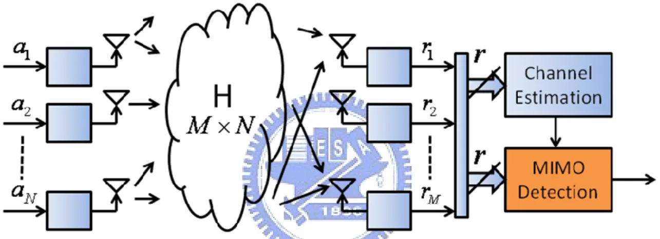
(16) Chapter 2 Review of the MIMO Detection Algorithms. Chapter 2 Review of the MIMO Detection Algorithms In this chapter, the MIMO system model will be given, and introduce some existing MIMO detection algorithms.. 2.1 MIMO System Model A MIMO system with N transmit antennas and M receive antennas is considered in this thesis as shown in Fig. 2.1. The discrete-time received signal r can be written as r  Hs  n ,. (1). where s denotes the N× 1 vector of the simultaneous transmitted symbols that selects from constellation C, and |C| denotes the constellation size. H is the M×N equivalent channel transfer matrix, n is the M× 1 complex white Gaussian noise vector with zero mean and variance of  n2 . In this thesis, the elements in H are assumed to be independent identically distributed (IID) complex Gaussian random variable with zero mean, where the dimension is under M  N. It is assumed that the receiver knows channel matrix H perfectly. This is shown that the ML detector is an optimum solution for the receiver in which the scheme detects all sub-stream symbols jointly by choosing. 4.

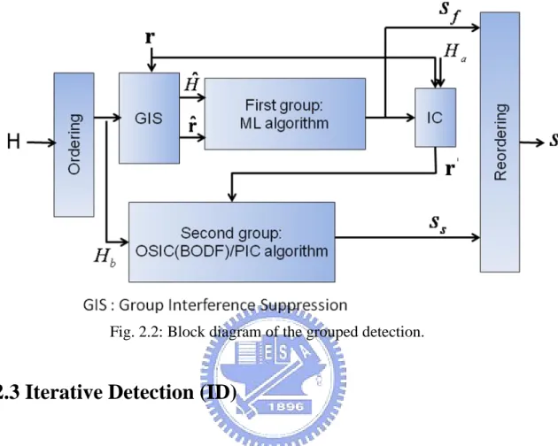
(17) Chapter 2 Review of the MIMO Detection Algorithms. the symbol vector which maximizes likelihood function. The above treatment is equivalent to the minimum Euclidean distance (MED) function in (2). 2. s  arg min r  Hsi , i. (2). where x denotes 2-norm of the vector x and s i denotes i-th candidate choosing from all possible combination of symbols. Note that the number of all combinations is |C|N. Nevertheless, the high computation-complexity ML scheme blocks the VLSI implementation. Several low-complexity detection algorithms [11-19] have been widely studied. Herein, we briefly review the complexity-oriented algorithms as follows.. Fig. 2.1: A MIMO system with N transmitters and M receivers.. 2.2 Grouped Detection (GD) The grouped detection algorithm [12] applies the ordering, GIS [13], ML algorithm to the first group symbols, interference canceling (IC), and BODF algorithm to the second group symbols as shown in Fig.2.2. The GIS not only plays the role of dividing symbols into two groups but also suppresses the performance influence of the low SNR signals. After ordering symbols, the ML detection algorithm at the first group is employed to detect higher SNR signals. Because of the property of the ML algorithm, we can detect symbols at the early stage and guarantee the performance without error propagation. The remaining symbols at the second group disturbed by high noise power 5.

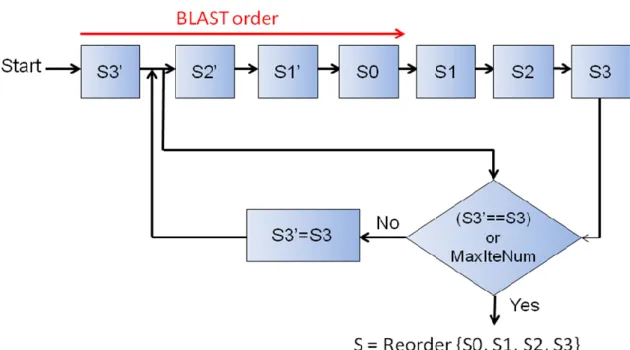
(18) Chapter 2 Review of the MIMO Detection Algorithms. can be detected by a suboptimal algorithm such as the BODF detection algorithm [7]-[10].. Fig. 2.2: Block diagram of the grouped detection.. 2.3 Iterative Detection (ID) The iterative detection algorithm detects symbols iteratively was proposed in [14], [15]. The traditional BODF algorithm detecting each symbol once propagates errors owing to the low-diversity symbols and thus greatly constraints the overall system performance. The algorithm detects symbols repeatedly in some specific sequence such that low-diversity symbols are detected by using decisions from high-diversity symbols to retrieve the high diversity gain. Enhancing diversity for all symbols can decrease error propagation. An example is provided in Fig. 2.3 to show the detection flow using the iterative detection [15].. 6.

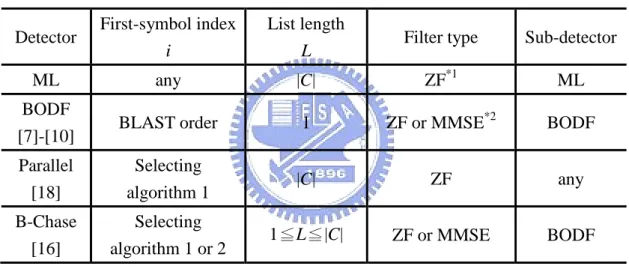
(19) Chapter 2 Review of the MIMO Detection Algorithms. Fig. 2.3: An Example of the iterative detection at 4 transmitted symbols.. 2.4 Chase Detection The Chase detection algorithm [16], [17] which shown in Fig. 2.4 determines which symbol detected first, list length, filter type, and sub-detector algorithm for the MIMO detection application. Many detection algorithms including ML, BODF, parallel [18], B-Chase and S-Chase can be derived from the Chase detection algorithm by adjusting the above four parameters. Table 2.1 shows how to generate the different detection algorithms. The B-Chase detection based on the BODF algorithm provides a tradeoff between the complexity and performance by choosing the list length. When the list length equals the constellation size, the performance of the B-Chase detection is close to that of the ML detection. Although the SD algorithm has better performance than the above Chase detector does, the SD detector shows larger computational complexity in [16]. For example, in [16], at BER=10-3, the SD and B-Chase algorithms respectively own the complexity of 57 RM/b and 18 RM/b, where RM/b represents the required number of real multiplications per detected bit. Hence, in this thesis, we 7.

(20) Chapter 2 Review of the MIMO Detection Algorithms. consider the Chase detection algorithm for complexity comparison instead of the SD algorithm.. Fig. 2.4: Block diagram of the Chase detection.. Table 2.1: Cases of the Chase detection algorithm Detector. First-symbol index i. List length L. Filter type. Sub-detector. ML. any. |C|. ZF*1. ML. BLAST order. 1. ZF or MMSE*2. BODF. Parallel [18]. Selecting algorithm 1. |C|. ZF. any. B-Chase [16]. Selecting algorithm 1 or 2. 1≦L≦|C|. ZF or MMSE. BODF. BODF [7]-[10]. *1. ZF : Zero forcing. *2. MMSE : Minimum mean square error. 2.5 GPIC Detection The generalized parallel interference cancellation (GPIC) detection algorithm [19] is similar to the Chase detection algorithm. The GPIC detection uses two PIC techniques; one is the same as that of the Chase detection algorithm, and another is referred to as a redetection scheme. Fig. 2.5 shows the block diagram of the GPIC detection. For the first PIC technique, the GPIC extends the number of the symbols 8.

(21) Chapter 2 Review of the MIMO Detection Algorithms. detected first compared with the Chase detection. In this case, the number of list lengths is the same as the number of all possible combinations of the symbols detected first. Then, the GPIC detection applies the redetection scheme to detect residual symbols, where the redetection scheme uses linear detection (LD) algorithm for lower computational complexity.. Fig. 2.5: Block diagram of the GPIC detection.. 9.

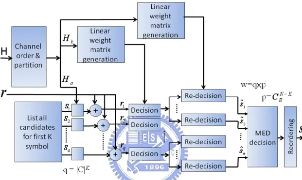
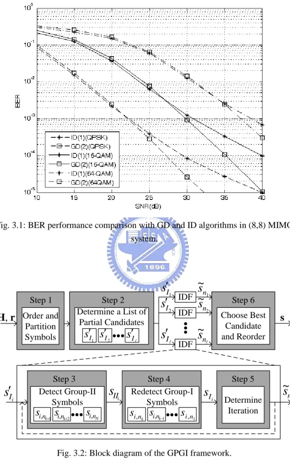
(22) Chapter 3 Generalized Parallel Grouped-Iterative (GPGI) MIMO Detection Framework. Chapter 3 Generalized Parallel Grouped-Iterative (GPGI) MIMO Detection Framework In this chapter, we develop the generalized parallel group-iterative (GPGI) framework. Through this framework, we not only generate several previously reported detection algorithms including BODF, GD, ID, B-Chase, GPIC(K,0) detection algorithms, but also propose a new flexible detection algorithm [20]. It is shown in Fig. 3.1 that the GD algorithm outperforms the ID algorithm at high SNR environment. On the other hand, the GD algorithm has weaker performance than the ID does at low SNR environment. We are motivated to take advantages of both algorithms in the following way to attain the low complexity and take into account of the satisfactory performance. Note that each GD and ID algorithm has higher computational complexity than the new one detection algorithm. The proposed GPGI framework can be performed by six steps as shown in Fig. 3.2. We partition all symbols into two groups referred to as group-I and group-II symbols by the GIS scheme and then apply iterative detection to the two group-symbols. In order to further improve performance, we generate more candidates to look for better solution.. 10.

(23) Chapter 3 Generalized Parallel Grouped-Iterative (GPGI) MIMO Detection Framework. Fig. 3.1: BER performance comparison with GD and ID algorithms in (8,8) MIMO system.. Step 1. H, r Order and Partition Symbols. sIi. 1. Step 2 Determine a List of Partial Candidates. sI sI 1. Step 3 Detect Group-II Symbols. si,nk1 si,nk2. sI sI. si,nN. 2. sIIi. 2. sI . s I . ~ sn ~ s. 1. IDF. n2. IDF. ~ sn. IDF. Step 4 Redetect Group-I Symbols. si,nk si,n. k1. si ,n. Step 6 Choose Best Candidate and Reorder. Step 5. sI i. Determine Iteration. 1. Fig. 3.2: Block diagram of the GPGI framework.. 11. s. ~ sni.

(24) Chapter 3 Generalized Parallel Grouped-Iterative (GPGI) MIMO Detection Framework. 3.1 Steps of GPGI Framework Each step is illustrated in the following. Step 1:. Order and partition all symbols into two groups. Group I has K symbols. {s n1 , s n2 , , s nk } with the highest order, and the residual (N-K) symbols {s nk 1 , s nk 2 , , s n N } are distributed to group II.. Step 2:. Determine a list of partial candidates { s I1 , s I 2 , , s I  } according to the MED. criterion for the group-I symbols, where sI i  [si,n1 si,n2  si,nk ]T , where xT denotes the transpose of x. Step 3:. Cancel the interference of r from the K symbols for each s I i to derive ri ,. and detect the remaining (N-K) symbols s II i  [si ,nk 1 si ,nk 2  si ,nN ]T . Step 4:. Cancel the interference of r from the (N-K) symbols for each s II i to derive. ri , and redetect the K symbols s I i  [ si ,nk si ,nk 1  si ,n1 ]T .. Step 5:. Determine whether the iterative operation is activated by detection algorithm.. If iteration is triggered, the GPGI framework will update the parameter values. When there is no iteration, we combine s I i and s II i into the i-th candidate ~sni . Step 6:. Choose the best hard decision ~s among the candidates { ~sn , ~sn , , ~sn } by 1. 2. . the MED criterion, and then reorder ~s into s.. 3.2 The Properties of GPGI Framework We treat steps 3~5 as an iterative decision feedback (IDF) block that detects two group symbols repeatedly. The operations of steps 1~3 are regarded as the GD 12.

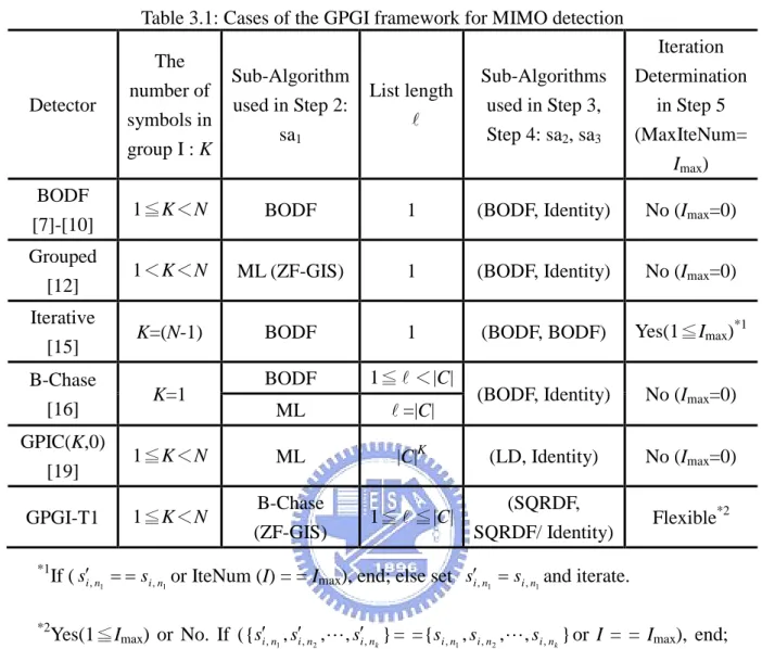
(25) Chapter 3 Generalized Parallel Grouped-Iterative (GPGI) MIMO Detection Framework. algorithm. We generate more candidates at step 2 and process each IDF in parallel. Due to three features of parallel, grouped and iterative, we name as the generalized parallel grouped-iterative (GPGI) detection framework. In order to configure different detection algorithms in the GPGI framework, three parameters and three sub-algorithms are defined in the following.  K: Number of symbols in group I whose range is 1  K<N.   : List length whose value is 1    |C|K.  Imax: Maximum number of iterations whose number is Imax  0. sa1, sa2, and sa3: Sub-detection algorithms used in step 2, 3, and 4, respectively. As shown in Table 3.1, while (K,  , Imax)= (1  K<N, 1, 0) and (sa1, sa2, sa3)=(BODF, BODF, Identity), the framework can generate the BODF algorithm in [7-10]. Note that identity means that we bypass the operations at this stage and feed the symbols directly to. the. next. step.. When. identity. used. at. step. 4,. we. assign. {si , n1 , si , n2 , , si , nk } = {si, n1 , si, n2 , , si, nk } . While (K,  , Imax)= (1<K<N, 1, 0) and (sa1, sa2,. sa3)=(ML, BODF, Identity), the framework can reduce to the GD algorithm in [12]. While (K,  , Imax)= (N-1, 1, Imax  1) and (sa1, sa2, sa3)=(BODF, BODF, BODF), the framework can generate the ID algorithm in [15]. While (K,  , Imax)= (1, 1   <|C|, 0) and (sa1, sa2, sa3)=(BODF, BODF, Identity), the framework can generate the B-Chase algorithm in [16]. While (K,  , Imax)= (1  K<N , |C|K, 0) and (sa1, sa2, sa3)=(ML, LD, Identity), the framework can reduce to the GPIC(K,0) algorithm in [19]. The generalized parallel interference cancellation (GPIC) algorithm [19] can be regarded as an extended type of the B-Chase algorithm which differs from the partition of the number of symbols and sa2. Hence, this framework can cover many conventional detection algorithms. Furthermore, one new proposed algorithm listed in the last row of Table 3.1 will be illustrated in the next chapter.. 13.

(26) Chapter 3 Generalized Parallel Grouped-Iterative (GPGI) MIMO Detection Framework. Table 3.1: Cases of the GPGI framework for MIMO detection. Detector. The number of symbols in group I : K. Sub-Algorithm used in Step 2: sa1. List length . Sub-Algorithms used in Step 3, Step 4: sa2, sa3. Iteration Determination in Step 5 (MaxIteNum= Imax). BODF [7]-[10]. 1≦K＜N. BODF. 1. (BODF, Identity). No (Imax=0). Grouped [12]. 1＜K＜N. ML (ZF-GIS). 1. (BODF, Identity). No (Imax=0). Iterative [15]. K=(N-1). BODF. 1. (BODF, BODF). Yes(1≦Imax)*1. B-Chase [16]. K=1. BODF. 1≦  ＜|C|. ML.  =|C|. (BODF, Identity). No (Imax=0). GPIC(K,0) [19]. 1≦K＜N. ML. |C|K. (LD, Identity). No (Imax=0). GPGI-T1. 1≦K＜N. B-Chase. (SQRDF,. 1≦  ≦|C|. (ZF-GIS). SQRDF/ Identity). Flexible*2. *1. If ( si, n1   si , n1 or IteNum (I) = = Imax), end; else set si, n1  si , n1 and iterate.. *2. Yes(1≦Imax) or No. If ( {si, n , si, n , , si, n } = = {si , n , si , n , , si , n } or I = = Imax), end; 1. 2. k. 1. 2. else set {si, n , si, n , , si, n } = {si , n , si , n , , si , n } and iterate. 1. 2. k. 1. 2. k. 14. k.

(27) Chapter 4 New Type GPGI-Based Detection Algorithm. Chapter 4 New Type GPGI-Based Detection Algorithm In this chapter, we explore the above framework by configuring three parameters as well as three sub-algorithms and then propose one new detection algorithm called GPGI-T1. After investigating the configuration parameters including K,  , Imax and three sub-algorithms including sa1, sa2, sa3, the GPGI framework can further optimize the complexity and performance. In the proposed algorithm, the ML sub-algorithm used at step 2 of the GD detection algorithm is replaced by the B-Chase sub-algorithm, where the performance of the B-Chase detection is close to that of the ML algorithm with low computational complexity. For low computational complexity and sub-algorithm regularity, we use the sorted QR decision feedback (SQRDF) algorithm [21] as sa2 and sa3 instead of the zero-forcing BODF sub-algorithm used in GD. Next, we give a wide range of parameters K,  , and Imax to trade off the complexity and performance.. 4.1 Implementation of GPGI-Type1 Each detailed design step implementation of the GPGI-T1 detection algorithm is summarized in Figs. 4.1, 4.2, and 4.3. Each corresponding design step is described in the following.. 15.

(28) Chapter 4 New Type GPGI-Based Detection Algorithm. Step 1: At the first step, we select K symbols with higher SNR to detect first by near-optimal algorithm such that error propagation can be alleviated. We resort the columns of channel matrix by 2-norm of the column. pi  h:, i. 2. for i = 1, 2,…, N.. (3). Where h :, i is the i-th column of H. According to the value of each pi , we can sort the values and obtain (4) p n1  p n2    p n N ,. (4). where {n1, n2, …, nN} denotes the detection order index. After permuting all symbols s, the channel matrix H, and identity matrix IN, we can recast the system function as follows. ~ r  H~s  n .. Where. ~ H  HΠ  [h n1 h n2 h nN ]. and. (5) ~s  T s  [s s  s ]T n1 n2 nN. ,. and. Π  [e n1 e n2  e n N ] . According to the values of K, ~s can be separated to two group. ~ symbols s I  [ sn1 sn2  snk ]T and s II  [snk 1 snk 2 snN ]T , and simultaneously H can. be considered as two sub-channels H and H  , where H   [h n1 h n2  h nk ] and H   [h nk 1 h nk 2  h n N ] .. Step 2: After symbol partition as shown in lines 1~5 of Fig. 4.1, we still cannot detect the corresponding symbols because they interfere with each other. In order to solve this problem and achieve lower complexity, we apply the GIS technique to channel matrix instead of the QR-decomposition. Then, we can divide original system into two lower dimensional sub-systems. In Fig. 4.2, we modify the ZF-GIS computation [13] to generate one sub-system used in Fig. 4.1 with lower complexity. Without loss of the generality, we illustrate the computation in (4,6) MIMO system, where (x,y) denotes 16.

(29) Chapter 4 New Type GPGI-Based Detection Algorithm. ~ x=N and y=M and set K=N/2 at this step. In this case, the ordered channel matrix H. can be written as ~ H  [h n1 h n2 h n3 h n4 ]  H H  h11 h12 h  21 h22  h31 h32  h41 h42  h51 h52   h61 h62. h13 h23 h33 h43 h53 h63. h14  h24  h34  . h44  h54   h64  . (6). In the proposed detection algorithm, we employ the matrix Hb to obtain a left null matrix Z of H  , where Hb is an ( N  K )  ( N  K ) square matrix on the bottom of H  and Z is an (M  N  K )  M matrix.. Z and Hb can be respectively expressed in. (7) and (8). 1 0 Z 0  0. 0 0 0. x 1, 1. 1 0 0 x 2, 1 0 1 0. x 3, 1. 0 0 1 x 4, 1. x 1, 2  x 2 , 2  , x 3, 2   x 4, 2 . (7). and  h53 Hb   h63. h54  . h64 . (8). We define xi=[xi,1 xi,2 …xi,(N-K)], and xi can be calculated via the following matrix computation. xTi  (HTb ) 1 hi,T:. for i = 1, 2, …, (M-N+K),. (9). where hi, : denotes the i-th row of H  . In this way, we can retrieve the left null matrix Z and then apply the Gram-Schmidt orthogonalization [22] to Z to obtain a row-orthogonal matrix L. Then, L is multiplied on both sides of (5) and we can derive the following equation as 17.

(30) Chapter 4 New Type GPGI-Based Detection Algorithm. ˆ s  nˆ , rˆ  H I. (10). ~ and H ˆ  LH with dimension of (M  N  K )  K . After the ZF-GIS where nˆ  L n. operation, we use the B-Chase detection algorithm [16] as sa1 to detect the sub-system in (10) for choosing better  candidates, where  ranges from 1 to |C|. Then, we can derive an ordered list of partial candidates { sI1 , sI 2 , , sI  } of the  candidates by the MED criterion in this sub-system. Steps 3, 4, and 5:. For convenience of illustration, the operations at steps 3, 4 and 5. are concurrently described. We just describe the operation of the i-th iterative decision feedback (IDF). At step 3 and 4 of the proposed work, we apply the SQRDF algorithm as sa2 and sa3 to detect two sub-systems in (11) and (12). ri  r  H sI i  H s II i  n ,. (11). ri  r  H s II i  H s I i  n  .. (12). The SQRDF algorithm can be divided into two parts: sorted QR decomposition (SQRD) and decision feedback (DF) whose pseudo code is listed in Fig. 4.3. Both parts can be computed using the algorithm in [17] with slightly modification. After the SQRD operation on H  , we can derive HΠ  QR , where Q  , R , Π  denote the unitary matrix, upper triangular matrix with positive and real diagonal elements, and permutation matrix, respectively. Next, we can obtain the vector d  which contains the reciprocal of the diagonal elements of R . After multiplying Q* on both sides of (11), the system can be changed to yi  Q*ri  Q*r  Q*HsI i  RsIIi  v ,. where sIIi  Π*s IIi  [si ,nk 1 si ,nk 2  si ,nN ]T , and where. (13). x* denotes the conjugate. transpose of x . s II i obtained from the DF operation in Fig. 4.3 can be expressed in 18.

(31) Chapter 4 New Type GPGI-Based Detection Algorithm. (14). N k    si ,nb  quan   yi,b  k   Rb k , j si ,n j  k  d b k ,b  k  , for b=N, N-1, …, K+1. j b  k 1   . (14). Where quan(x) denotes the quantization function which quantizes the value x to the nearest constellation point. The symbols s II i can be obtained by reordering s II i . Similarly, at step 4, we can obtain following equations in (15) and (16). yi  Q*ri  Q*r  Q*Hs IIi  RsI i  v .  si , nc  quan   y i , k  c 1  . (15). k    R k  c 1, j si , nk  j 1 d k  c 1, k  c 1  , for c=1, 2, …, K. (16) j  k c  2  . Where H Π   Q R  and sI i  Π*s I i  [si ,nk si ,nk 1  si ,n1 ]T . The maximum iterative number of Imax affects the computational complexity. The initial iterative number I is set to zero. When executing step 4 once, I is increased by one. If s I i equals s I i or I equals Imax, we obtain the candidate ~sni  [s I i s IIi ]T . Otherwise, let sI i  s I i and repeat steps 3 and 4. Note that if Imax=0, there is no need to deal with the sub-system of (12), and the operation of (15) and (16) can be skipped. Step 6: At the last step, we choose the final hard decision ~s according to the MED criterion among the candidates { ~sn , ~sn , , ~sn }. The MED of the i-th candidate is 1. . 2. ~ obtained by  i || r  H~si ||2 . According to the permutation matrix  at step 1, we. rank the detected symbols ~s to obtain the final symbols s. In terms of algorithm flexibility, when K=1, the GPGI-T1 algorithm can performs as the combination of the Chase and ID algorithms. When  =1, the GPGI-T1 algorithm reduces to the combination of the GD and ID algorithms. When Imax=0, the GPGI-T1 algorithm reduces to the combination of the Chase and GD algorithms.. 19.

(32) Chapter 4 New Type GPGI-Based Detection Algorithm FUNCTION: GPGI-T1 Detection Algorithm INPUT: (H, r, M, N, C, K,  , Imax) OUTPUT: (s). 1. for i = 1 to N , pi = ||h:, i||2 end 2. Π = N×N permutation matrix that sorted by pi from IN 3. 4. 5. 6. 7.. ~ H  HΠ ~ H  = first K columns of H ~ H = last (N-K) columns of H ˆ , rˆ ] = ZF-GIS( H , H , r , K ) [H ˆ , rˆ , C,  ) [ s , s ,, s ] = B-Chase( H I1. I2. I. 8. [ Q, R , d, Π ] = SQRD( H , p , Π ) 9. u  Q * r 10. v  Q * H  11. [ Q, R , d, Π  ] = SQRD( H , p, Π ) 12. 13.. u   Q * r v  Q * H. 14. Emin = ∞ 15. for i = 1 to  , 16. 17.. I=0 while (I < Imax) & ( sI  s I ), i. i. sI  s I. 18. 19. 20. 21. 22.. if I  0,. 23. 24. 25.. I=I+1 End. 26.. i= 0. 27. 28.. for j = 1 to M,. 29. 30. 31.. end. i. y  u  vsI. i. end. i. s II = DF( R, d, y, Π, N-K) i. y  u  vs II. i. s I = DF( R , d , y , Π , K) i. ei  r  Hs I  Hs II i. i.  i   i  | ei, j | 2. if  i < Emin , if  i < Emin ,. end. Emin =  i ~s  [s s ]T I II i. i. 32. end 33. end 34. s  Π~s Fig. 4.1: Processing pseudo code for the implementation of the GPGI-T1 detection algorithm for Imax≧1.. 20.

(33) Chapter 4 New Type GPGI-Based Detection Algorithm FUNCTION: ZF-GIS INPUT: ( H , H  , r, K). ˆ , rˆ ) OUTPUT: ( H. 1. H = (N-K)×(N-K) matrix at the bottom of H 2. W  (HTb ) 1 3. for i = 1 to (M-N+K), end x Ti   Whi,T: b. 4. X = [x1 x2 … xM-N+K]T 5. Z = [IM-N+K  X] 6. L = GSO(Z) 7. Hˆ  LH 8. rˆ  Lr Fig. 4.2: Processing pseudo code for the proposed modified GIS implementation.. FUNCTION: DF INPUT: ( R, y , d, Π, J ). OUTPUT: ( s ). 1. for i = 1 to J 2. t  ij11 ri , j s j 3.. si  quan (( yi  t ) d i ). 4. end 5. s  Πs. Fig. 4.3: Processing pseudo code for the proposed DF implementation that modified from [17].. 4.2 Reducing Complexity Highlight There are two schemes to lower the computational complexity. First, we reduce complexity by reusing tentative computations.  Observing (13) and (15), we can reuse tentative calculations for parallel and iterative computing such that we just compute the SQRD function on H and H  , Q*r , Q* H , Q*r , and Q* H once..  Observing (3), the 2-norm of each column of H can be reused in the computations of the SQRD function. 21.

(34) Chapter 4 New Type GPGI-Based Detection Algorithm. Second, we reduce complexity by avoiding unnecessary computations.  When the input symbols are the same as that at the last iteration, we can skip the calculations in the following iterations. That mean we do not need to reach the maximum iteration number Imax in each IDF.  We use pruning and threshold-tightening strategy given in [16] to generate a threshold Emin which records the last time MED values of other candidates. When the Euclidean distance is greater than Emin during the process, the computation can be terminated. Using the above two schemes, we can alleviate the computational complexity, where the complexity analysis of the GPGI-T1 algorithm will be debated in detail in the following chapter.. 22.

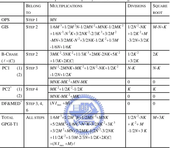
(35) Chapter 5 Complexity Analysis, Simulation Results, and Implementation. Chapter 5 Complexity Analysis, Simulation Results, and Implementation This chapter demonstrates the complexity and performance of the GPGI-T1 detection algorithm and shows the comparison results with the existing detection schemes including the BODF, GD, ID, B-Chase algorithms and GPIC(K,0) detection algorithm. We use the GPGI-T1(K,  , Imax) to denote the GPGI-T1 algorithm with K symbols distributed to group I, list length  and maximum iteration Imax. Moreover, the B-Chase(  ) denotes the ZF B-Chase algorithm with list length  , and the GPIC(K,E) denotes the GPIC algorithm with K symbols in group I and E error symbols in group II.. 5.1 Complexity Analysis In Table 5.1, we summarize the number of complex multiplications, complex divisions and square roots required by the GPGI-T1 algorithm. The GPGI-T1 algorithm includes the order and partition symbols (OPS), GIS, B-Chase used in sub-system, precomputation1 (PC1), precomputation2 (PC2) and the combination of DF and MED (DF&MED) of the design steps. PC1(1) and PC1(2) correspond to the operations of lines 8 and 9-10 of Fig. 4.1, respectively. Similarly, PC2(1) and PC2(2) represent the operations of lines 11 and 12-13 of Fig. 4.1, respectively. Although the computations of 23.

(36) Chapter 5 Complexity Analysis, Simulation Results, and Implementation. division and square root are more complex than those of multiplications, the number of divisions and square roots is much less than the number of multiplications in the GPGI-T1 and others algorithms. Therefore, the complexity is measured by the sum of complex multiplications, divisions and square roots in the worst case. The multiplication of a number and a constellation point can be implemented by scaled integers [23] such that we can reduce the number of multiplications. For simplicity, we assume that the number of transmitters is an even integer and K=N/2 in the GPGI-T1 algorithm, and the channel matrix changes during every symbol period. That means we process all computations at each symbol period. The comparisons of the worst-case computational complexity of the GPGI-T1 algorithm, B-Chase scheme, and GPIC(1,0) algorithm are tabulated in Table 5.2. When M=N, the complexity order of the GPGI-T1, B-Chase and GPIC algorithms are O(47/24N3), O(11/3N3) and O(4N3) respectively. Herein, we do not formulate the complexity of the GD and ID algorithms since both algorithms require more computational complexity than the B-Chase detection, where the complexity of the GD algorithm is exponential time of the number of first-group symbols and the complexity of the ID algorithm almost doubles that of the BODF algorithm (B-Chase(1)) mentioned in [15]. It is emphasized again that since the SD detector shows larger computational complexity as addressed in [16], for example, at BER=10-3, the SD and B-Chase algorithms respectively own the complexity of 57 RM/b and 18 RM/b, we only consider the Chase detection algorithm for complexity comparison instead of the SD algorithm.. 24.

(37) Chapter 5 Complexity Analysis, Simulation Results, and Implementation. Table 5.1: Computational complexity of the GPGI-T1 algorithm BELONG. MULTIPLICATIONS. DIVISIONS. TO. SQUARE ROOT. OPS. STEP 1. MN. GIS. STEP 2. 1/6M 3+1/2M 2N-1/2MN 2+MNK-1/2MK 2 1/2N 2-NK M-N+K +1/6N 3-N 2K+3/2NK 2-2/3K 3+3/2M 2 +1/2K 2+M -MN+3/2MK-N 2+3/2NK-1/2K 2+1/3M -3/2N+3/2K -1/6N+1/6K. B-CHASE (  =|C|). STEP 2. 3MK 2-3NK 2+11/3K 3+2MK-2NK+5K 2 +1/3K+2K|C|. 1/2K 2 +3/2K. 2K. MN 2-2MNK+MK 2+1/2N 2-NK+1/2K 2 -1/2N+1/2K. N-K. N-K. MNK-MK 2+MN-MK. 0. 0. MK +1/2K -1/2K. K. K. MNK-MK 2+MK. 0. 0. (N I max +M) . 0. 0. 1/6M 3+1/2M 2N+1/2MN 2+MNK +5/2MK2+1/6N 3-N 2K-3/2NK 2+3K 3 +3/2M 2+MN+7/2MK-1/2N 2-3/2NK +11/2K 2+1/3M-2/3N+1/2K+2K|C| +(N I max +M) . 1/2N 2-NK + K 2+ M -1/2N+3 K. M+3K. PC1. PC2. (1) STEP 3 (2) *. (1) STEP 4 (2). DF&MED* STEP 3, 4,. 2. 2. 6 TOTAL GPGI-T1. ALL STEPS. *. When Imax equals zero, the computational complexity of PC2 is equal to zero and the multiplication complexity of DF&MED is changed to (M+N-K)  . Table 5.2: Complexity comparison among the proposed GPGI-T1 and conventional algorithms ALGORITHM. MULTIPLICATIONS/DIVISIONS/SQUARE ROOTS. B-CHASE. 3MN 2+2/3N 3+2MN+7/2N 2+23/6N+2N . GPIC(1,0). 4MN 2-4MN+N 2+3/2M-2N+1+MN|C|. GPGI-T1. 1/6M 3+1/2M 2N+13/8MN 2-1/3N 3+3/2M 2+11/4MN +3/8N 2+7/3M+25/12N+N|C|+( N I max +M)  *2. *1. *1. When 1<  <|C|, the additional computation complexity of 1/6N 3+3/2N 2+4/3N is needed.. *2. In this case, N is an even integer and K=N/2.. 25.

(38) Chapter 5 Complexity Analysis, Simulation Results, and Implementation. 5.2 Simulation Results On the other hand, we show simulation results to sustain the performance of the GPGI-T1 detection algorithm. The simulation environment is assumed Rayleigh flat-fading channel and no correlation between sub-channels. The performance measurement targets at the SNR that reaches BER=10-3. Fig. 5.1 shows the performance of the GPGI-T1 algorithm with different K and  in (8,8) system with 16-QAM inputs. We can find that the performance with larger K is better than that with smaller K under the same  . In this case, the complexity of the GPGI-T1 algorithm with K=6 approximately doubles with K=2 under the same  , and the range of performance of the GPGI-T1 algorithm with K=6 is narrow. In order to trade off the complexity and performance, we prefer to choose K in the range from 2 to N/2. Fig. 5.2 shows the performance of the GPGI-T1 algorithm with different Imax and  in (8,8) system with QPSK inputs. The performance of the GPGI-T1 algorithm can be improved by increasing Imax under the same  . We set K=N/2 and suitable value of Imax in the GPGI-T1 algorithm to compare with the existing detection algorithms. Figs. 5.3-5.10 show the performance in (4,4), (6,6), (8,8), and (4,6) systems. Figs. 5.3, 5.5, 5.7, and 5.9 use the constellation of QPSK, and Figs. 5.4, 5.6, 5.8, and 5.10 use the constellation of 16-QAM. From the comparison results, we can find out the BER performance of the GPGI-T1 algorithm can be significantly enhanced by slightly increasing the list length  . For example, GPGI-T1(2,2,1) outperforms GPGI-T1(2,1,1) by 3.3 dB and 3 dB with. respect to QPSK and 16-QAM inputs in (4,4) system, and just increases complexity 3.3% and 2.8%. The better performance can be obtained with longer list length; GPGI-T1(2,16,1) outperforms GPGI-T1(2,1,1) by 5 dB with 16-QAM inputs. On the other hand, better BER performance can be obtained by increasing Imax under the same 26.

(39) Chapter 5 Complexity Analysis, Simulation Results, and Implementation. list length. For example, in (8,8) system with QPSK inputs, GPGI-T1(4,4,3) outperforms GPGI-T1(4,4,0) and GPGI-T1(4,4,1) by 1.3 dB and 0.3 dB, respectively. In summary, the computational complexity and BER performance of the GPGI-T1 algorithm depends on these parameters given above. The smaller K,  , Imax, and simplified sub-algorithm achieve low complexity. Otherwise, the higher K,  , Imax, and better sub-algorithm attain better performance.. Fig. 5.1: BER performance of the GPGI-T1 algorithm with different K and  in (8,8) MIMO system with 16-QAM inputs.. 27.

(40) Chapter 5 Complexity Analysis, Simulation Results, and Implementation. Fig. 5.2: BER performance of the GPGI-T1 algorithm with different Imax and  in (8,8) MIMO system with QPSK inputs.. Fig. 5.3: BER performance of the GPGI-T1 algorithm and conventional algorithms in (4,4) MIMO system with QPSK inputs.. 28.

(41) Chapter 5 Complexity Analysis, Simulation Results, and Implementation. Fig. 5.4: BER performance of the GPGI-T1 algorithm and conventional algorithms in (4,4) MIMO system with 16-QAM inputs.. Fig. 5.5: BER performance of the GPGI-T1 algorithm and conventional algorithms in (6,6) MIMO system with QPSK inputs.. 29.



(44) Chapter 5 Complexity Analysis, Simulation Results, and Implementation. Fig. 5.10: BER performance of the GPGI-T1 algorithm and conventional algorithms in (4,6) MIMO system with 16-QAM inputs.. 5.3 Complexity-Performance Tradeoff Next, we show the complexity-performance tradeoff of the GPGI-T1, B-Chase, and GPIC(1,0) algorithms in Figs. 5.11 and 5.12. In (8,8) system, GPGI-T1(4,1,3) not only reduces the complexity of 38.1% and 33.9% but also gains 9.5 dB and 10 dB compared with the BODF algorithm (B-Chase(1)) with respect to QPSK and 16-QAM inputs, respectively. GPGI-T1(4,16,3), GPGI-T1(4,4,3), and GPGI-T1(4,2,3) reduce the complexity of 21.5%, 36.8%, and 39.3% while falling 0.3 dB, 0.4 dB, and 0.8 dB short of the B-Chase(16) algorithm with 16-QAM inputs respectively. In other configurations with M=N, the comparison of complexity and performance has behavior similar to that of the above analysis trend. On the other hand, in (4,6) system, the GPGI-T1 algorithm has comparable performance and less computational complexity. We do not present the. 32.

(45) Chapter 5 Complexity Analysis, Simulation Results, and Implementation. comparison with GD and ID here since both algorithms require more computational complexity compared with the corresponding cases of the GPGI-T1 algorithm, and have poor BER performance. Therefore, from the complexity and performance analysis, the GPGI-T1 algorithm attains better complexity-performance tradeoff at the slight penalty of BER performance degradation compared with the B-Chase and GPIC(1,0) detection algorithms. Moreover, the GPGI-T1 algorithm has the lowest complexity in all cases under M=N and provides adjustable performance for different user’s requirements.. Fig. 5.11: Complexity-performance trade-off of the GPGI-T1, B-Chase and GPIC(1,0) algorithms with QPSK inputs.. 33.

(46) Chapter 5 Complexity Analysis, Simulation Results, and Implementation. Fig. 5.12: Complexity-performance trade-off of the GPGI-T1, B-Chase and GPIC(1,0) algorithms with 16-QAM inputs.. 5.4 VLSI Implementation In this section, we begin to show that how implement a multi-mode MIMO detector using the proposed GPGI-T1 algorithm. We replace the block diagram of the GPGI framework in Fig. 3.2 to that of our proposed GPGI-T1 algorithm in Fig. 5.13. Q2*H1 SQRD H2=Q2R2. Q2*r Q1*H2. H. Qrder & Parteition. SQRD H1=Q1R1. ZF-GIS. IC. DF. MED & Reorder. IC. DF. MED & Reorder. IC. DF. MED & Reorder. Q1*r. H'=ZH1 r'=Zr. B-Chase Algorithm. Fig. 5.13: Block diagram of the GPGI-T1 algorithm. 34. Choose the best candidate. s.

(47) Chapter 5 Complexity Analysis, Simulation Results, and Implementation. Besides, the channel matrix H is the same for each frame. It means that we just compute the variable that only related to H once each frame. So, we divide the detection flow of the GPGI-T1 algorithm into two parts, preprocessing part and decision part. The preprocessing part computes just once when the channel matrix H is unchanged, and the decision part operates for each symbol period. In this thesis, we just implement the decision part, where the maximum iteration Imax is equal to zero. The block diagram of the GPGI-T1 implementation is shown in Fig. 5.14.. r. H. Preprocessing Part. Qrder & Parteition. Decision Part. SQRD H2=Q2R2. V=Q2*H1. ZF-GIS. H'=ZH1. PreU Order H'. PreB-Chase. B-Chase Algorithm. DF & MED. s. Fig. 5.14: Block diagram of the implementation of the GPGI-T1 algorithm.. Moreover, we would like to design a multi-mode GPGI-T1 detector which can work in many practical conditions including (2,2) and (4,4) MIMO system with QPSK, 16-QAM, and 64-QAM inputs. We design the MIMO detector with power-aware feature in (4,4) MIMO system. Before designing hardware architecture, we simulate the BER performance of the floating-point GPGI-T1 algorithm and the modified fixed-point GPGI-T1 algorithm in (4,4) MIMO system with 64-QAM inputs, the critical mode in our implementation, as shown in Fig. 5.15. The modified GPGI-T1 algorithm changes the MED function from 2-norm to 1-norm. We can find that GPGI-T1(2,8,0) is a setting candidate for the trade-off of the BER performance and computational complexity. Therefore, we set that the maximal list length equals eight in the multi-mode GPGI-T1 detector, and the maximal input word length equals ten bits. Table 5.3 illustrates how to attain multi-mode BER performance by adjusting the parameter  . 35.

(48) Chapter 5 Complexity Analysis, Simulation Results, and Implementation. The pipeline architecture of the multi-mode GPGI-T1 detector is depicted in Fig. 5.16. The two-group input buffers are used to store inputs and process data simultaneously. The Pre-U and Pre-B-Chase parts implemented by multiply Accumulate (MAC) unit process the reused variables for B-Chase and DF&MED parts. The B-Chase part is divided to four stages. The former two stages are in charged of parallel search and Euclidean distance calculation. The latter two stages play the role of sorting network implemented by Bitonic sort. The DF&MED part is divided to four stages including interference cancellation (IC), decision feedback 1 (DF1), decision feedback 2 (DF2), and minimum Euclidean distance (MED). The IC stage cancels the interference from the two symbols obtained by B-Chase. The DF1 and DF2 stages decide another two symbols and calculate the temporary variable for Euclidean distance calculation. The MED stage calculates the final Euclidean distance and stores the symbols with MED after comparison.. 36.

(49) Chapter 5 Complexity Analysis, Simulation Results, and Implementation. Fig. 5.15: BER performance of the GPGI-T1 algorithm and B-Chase algorithm in (4,4) MIMO system with 64-QAM inputs.. Table 5.3: Performance selection by choosing different list length 4×4. Antenna Modulation. QPSK. 16-QAM. 64-QAM. BER Performance. Close to optimal. Close to optimal. Close to optimal. Close to optimal / Suboptimal. Close to optimal / Suboptimal. Close to optimal / Suboptimal. List length . 2. 1. 4. 1. 8. 1. 37.

(50) Chapter 5 Complexity Analysis, Simulation Results, and Implementation. Fig. 5.16: Pipeline architecture of the multi-mode GPGI-T1 detector.. Concerning the chip implementation, the cell-based design flow with Artisan standard cell library is adopted and the multi-mode GPGI-T1 detector has been implemented in TSMC 0.18-um CMOS process. The Synopsys Design Compiler is used to synthesize the RTL design of the proposed detector and Cadence SOC Encounter is adopted for placement and routing (P&R). The Synopsys PrimePower is used to analyze the power consumption. The active chip layout area of the proposed multi-mode GPGI-T1 detector as shown in Fig. 5.17 is 1.41 mm × 1.39 mm. Table 5.4 summarizes the chip characteristics of the multi-mode GPGI-T1 detector. Table 5.5 summarizes the supplied modes and the respective power consumption of our chip design. It can work in nine modes, where three and six modes belong to (2,2) and (4,4) systems, respectively. The multi-mode functions of the GPGI-T1 detector has been proved by post-layout simulation verification as shown in Fig 5.18. Table 5.6 provides a comprehensive comparison of the relevant ASIC implementations for MIMO detection. In [23] and [24], the BER performance of the implementation algorithms is optimal or close to optimal, respectively, but the power consumption is large. An implementation of the BODF algorithm by square root method [9] which shows low computational complexity but poor BER performance was proposed in [25]. The above chip design [25] including preprocessing part has better power efficiency than the SD implementation [23], [24], where the power efficiency is 38.

(51) Chapter 5 Complexity Analysis, Simulation Results, and Implementation. defined as the ratio of the normalized throughput to the normalized power. Our implementation of the GPGI-T1 algorithm has best power efficiency compared with other implementation designs. For example, in (4,4) MIMO system with 16QAM inputs, our design shows seven times the power efficiency of the implementation in [24]. Furthermore, our design possesses low-complexity computation and multi-mode implementation with better power efficiency compared with other reference designs.. Fig. 5.17: Chip layout of the multi-mode GPGI-T1 detector.. 39.

(52) Chapter 5 Complexity Analysis, Simulation Results, and Implementation. Table 5.4: Chip characteristics of the multi-mode GPGI-T1 detector Power Supply. 1.8 V. Max. Clock. 100 MHz. Max. Power. 177 mW. Gate Count. 141 K. Active Chip Area. 1.41 mm × 1.39 mm. Process Technology. TSMC 0.18 um CMOS. Table 5.5: Supplied modes of the GPGI-T1 chip implementation 2×2. Antenna. 4×4. Modulation. QPSK. 16-QAM. 64-QAM. QPSK. 16-QAM. 64-QAM. BER. Close to. Close to. Close to. Close to. Close to. Close to. Performance. optimal. optimal. optimal. optimal / Suboptimal. optimal / Suboptimal. optimal / Suboptimal. Throughput. 50Mbps. 100Mbps. 150Mbps. 100Mbps. 200Mbps. 300Mbps. Power (mW). 79. 95. 126. 118/116. 137/130. 177/161. Fig. 5.18: Post-layout simulation of the multi-mode GPGI-T1 detector. 40.

(53) Chapter 5 Complexity Analysis, Simulation Results, and Implementation. Table 5.6: Comparison of ASIC implementation for MIMO detection IEEE JSSC [23] Design 1. IEEE JSSC [23] Design 2. IEEE JSAC [24]. JVLSI Signal Processi ng [25] *. Proposed Work. Antenna. 4×4. 4×4. 4×4. 4×4. 4×4. Modulation. 16-QAM. 16-QAM. 16-QAM. QPSK. QPSK/16-QAM /64-QAM. Detector. SD. SD. K-best SD. BODF. GPGI-T1. BER performance. Optimal. Close to optimal. Close to optimal. Suboptimal. Close to optimal / Sub-optimal. Technology. 0.25 um. 0.25 um. 0.35 um. 0.35 um. 0.18 um. Cate Count. 117 K +preproc.. 50 K +preproc.. 91 K +preproc.. 190 K. 141 K +preproc.. Max. Clock. 51 MHz. 71 MHz. 100 MHz. 80 MHz. 100 MHz. Throughput. 73 Mbps @20 dB. 169 Mbps @20 dB. 53.3 Mbps. 128 Mbps. 100/200/300 Mbps. Power. 360 mW @2.5 V. N/A. 626 mW @2.8 V. 608 mW @2.7 V. Power. 0.391. Efficiency. Mbps/mW. N/A. 0.206. 0.474. Mbps/Mw. Mbps/m W. *. Close to optimal. Suboptimal. 118/137 /177 mW. 116/130 /161 mW. 0.847. 0.862. /1.46/1.69 /1.54/1.86 Mbps/m Mbps/m W W. Note that the implementation includes the preprocessing part. If the preprocessing part. is removed, the power consumption will decrease greatly.. 41.

(54) Chapter 6 Conclusion and Future Work. Chapter 6 Conclusion and Future Work In this thesis, the GPGI framework that generates many MIMO detection algorithms has been presented. Based on the GPGI framework, we propose the GPGI-T1 detection algorithm that trades off the complexity and performance by modifying the number of symbols detected first, the list length and the numbers of maximum iterations. The GPGI-T1 detection algorithm significantly reduces the multiplication complexity and has comparable BER performance compared with the existing detection algorithms. For example, in (8,8) system with 16-QAM inputs, GPGI-T1(4,1,3) can reduce the multiplication complexity by 33.9% and outperform 10 dB compared with the BODF detection at low complexity end. At high performance end, GPGI-T1(4,16,3) and GPGI-T1(4,2,3) can reduce the multiplication complexity by 21.5% and 39.3% at the penalty of 0.3 dB and 0.8 dB loss compared with the B-Chase(16) detection, respectively. With the features of low complexity, satisfactory BER performance and parallel processing, the GPGI-T1 algorithm is suitable for modern high-speed communication systems. According to the proposed GPGI-T1 algorithm, we implement a multi-mode MIMO detector using TSMC 0.18um process CMOS. The resulting implementation supports QPSK, 16-QAM, and 64-QAM modulation modes, and can work in nine modes, where three and six modes belong to (2,2) and (4,4) systems, respectively. Importantly, the resulting MIMO detection implementation possesses the comparable power efficiency among five 42.

(55) Chapter 6 Conclusion and Future Work. ASIC designs.. 43.

(56) Bibliography. Bibliography [1] G. J. Foschini, “Layered space-time architecture for wireless communication in a fading environment when using multi-element antennas,” Bell Labs Tech. J., vol. 1, no. 2, pp. 41-59, Autumn 1996. [2] I. E. Telatar, “Capacity of multi-antenna Gaussian channels,” Eur. Trans. Telecommum., vol.10, no. 6, pp. 585-595, Nov. 1999. [3] A. van Zelst and T. C. W. Schenk, “Implementation of a MIMO OFDM-based wireless LAN system,” IEEE Trans. Signal Processing, vol. 52, no. 2, pp. 483-494, Feb. 2004. [4] E. Viterbo and J. Boutros, “A univrsal lattice decoder for fading channels,” IEEE Trans. Inform. Theory, vol. 45, no. 5, pp. 1639–1642, Jul. 1999. [5] E. Agrell, T. Eriksson, A. Vardy, and K. Zeger, “Closest point search in lattices,” IEEE Trans. Inf. Theory, vol. 48, no. 8, pp. 2201–2214, Aug. 2002. [6] M. O. Damen, H. El Gamal, and G. Caire, “On maximum-likelihood detection and the search for the closest lattice point,” IEEE Trans. Inf. Theory, vol. 49, no. 10, pp. 2389–2402, Oct. 2003. [7] P. W. Wolniansky, G. J. Foschini, G. D. Golden, and R. A. Valenzuela, “V-BLAST: An architecture for realizing very high data rates over the rich-scattering wireless channel,” in Proc. ISSSE, Sep.-Oct. 1998, pp. 295–300.. 44.

(57) Bibliography. [8] G. D. Golden, C. J. Foschini, R. A. Valenzuela, and P. W. Wolniansky, “Detection algorithm and initial laboratory results using V-BLAST space-time communication architecture,” Electron. Letters., vol. 35, no. 1, pp. 14–16, Jan. 1999. [9] B. Hassibi, “An efficient square-root algorithm for BLAST,” in Proc. IEEE Conf. Acoustics, Speech, Signal Processing (ICASSP), Jun. 2000, vol. 2, pp. 737-740. [10] Jacob Benesty, Yiteng Huang, and Jingdong Chen, “A fast recursive algorithm for optimum sequential signal detection in a BLAST system,” IEEE Trans. Signal Processing, vol.51, no.7, pp. 1722-1730, July 2003. [11] W. Choi, R. Negi, J. Cioffi, “Combined ML and DFE decoding for the V-BLAST system,” in Proc. IEEE Conf. Commun. (ICC), Jun. 2000, vol. 3, pp. 1243-1248. [12] L. Yang, M. Chen, S. Cheng, and H. Wang, “Combined maximum likelihood and ordered successive interference cancellation grouped detection algorithm for multistream MIMO,” in Proc. IEEE Int. Sym. Spread Spectrum Tech. and Appl., Aug.-Sep. 2004, pp. 250-254. [13] Vahid Tarokh, Ayman Naguib, Nambi Seshadri, and A. Robert Calderbank, “Combined array processing and space-time coding” IEEE Trans. Inform. Theory, vol. 45, no. 4, pp. 1121-1128, May 1999. [14] Cong Shen, Hairuo Zhang, Lin Dai, and Shidong Zhou, “Detection algorithm improving V-BLAST performace over error propagation” Electronic Letters, vol. 39, no. 13, pp. 1107-1108, June 2003. [15] D. Li, L. Cai and H. Yang, “New iterative detection algorithm for V-BLAST,” in Proc. IEEE Vehicular Technol. Conf. (VTC), Sep. 2004, vol. 4, pp.2444-2448. 45.

(58) Bibliography. [16] D. W. Waters and J. R. Barry, “The Chase family of detection algorithms for multiple-input multiple-output channels,” IEEE Trans. Signal Processing, vol.56, no.2, pp. 739-747, Feb. 2008. [17] D. W. Waters and J. R. Barry, “The sorted-QR chase detector for multiple-input multiple-output channels,” in Proc. IEEE Wireless Commum. and Networking Conf. (WCNC), Mar. 2005, vol. 1, pp. 538-543. [18] Y. Li and Z. Luo, “Parallel detection for V-BLAST system,” in Proc. IEEE Conf. Commun. (ICC), May. 2002, vol. 1, pp.340-344. [19] Z. Luo, M. Zhao, S. Liu, and Y. Lin, “Generalized parallel interference cancellation with near-optimal detection performance,” IEEE Trans. Signal Processing, vol.56, no.1, pp. 304-312, Jan. 2008. [20] D. Y. Wu and L. D. Van, "A grouped-iterative framework for MIMO detection," in Proc. IEEE Vehicular Technol. Conf. (VTC), Sep. 2008, accepted, Calgary, Canada. [21] D. Wübben, R. Böhnke, J. Rinas, V. Kühn and K. Kammeyer, “Efficient algorithm for decoding layered space-time codes,” Electronic Letters, vol.37, no. 22, pp.1348-1350, Oct 25, 2001. [22] G.H. Golub and C.F. Van Loan., Matrix Computations, third edition, Baltimore, MD: Johns Hopkins University Press, 1996. [23] A. Burg, M. Borgmann, M. Wenk, M. Zellweger, W. Fichtner, and H. Bölcskei, “VLSI implementation of MIMO detection using the sphere decoding algorithm,” IEEE J. Solid-State Circuits, vol. 40, no. 7, pp.1566–1577, Jul. 2005. [24] Z. Guo and P. Nilsson, “Algorithm and implementation of the K-Best sphere decoding for MIMO detection,” IEEE J. Selected Areas in Communication, vol. 24, no. 3, pp.491–503, Mar. 2006. 46.

(59) Bibliography. [25] Z. Guo and P. Nilsson, “A VLSI architecture of the square root algorithm for V-BLAST detection,” J. VLSI Signal Processing, vol. 44, pp.219–230, 2006.. 47.

(60) Autobiography. Autobiography 吳廸優，高雄人，生於公元 1984 年 1 月 30 日。先後畢業於高雄縣立登發國民小學、高雄縣立文山中學、國立鳳山高級中學及國立成功大學數學系。2006 年 9 月進入國立交通大學資訊學院資訊科學與工程研究所碩士班就讀。其研究興趣為無線通訊系統、VISI 訊號處理、SOC 平台之軟硬體整合設計與系統分析，碩士論文題目為應用於多輸入多輸出通道之低複雜度多模式訊號偵測演算法與超大型積體電路實現。. 48.

(61)