A Genetic Algorithm for the Bandwidth Calculation Problem in Mobile Ad Hoc Networks
19
0
0
全文
(2) 1. Introduction A mobile ad-hoc network (MANET) is formed by a group of mobile hosts (or called mobile nodes) without an infrastructure consisting of a set of fixed base stations. A mobile host in a MANET can act as both a general host and a router, i.e., it can generate as well as forward packets. Two mobile hosts in such a network can communicate directly with each other through a single -hop route in the shared wireless media if their positions are close enough. Otherwise, they need a multi-hop route to finish their communications. In a multi-hop route, the packets sent by a source are relayed by several intermediate hosts before reaching their destination. MANETs are found in applications such as short-term activities, battlefield communications, disaster relief situations, and so on. Undoubtedly, MANETs play a critical role in environment where a wired infrastructure is neither available nor easy to establish. The research of MANETs has attracted a lot of attentions recently. In particular, since MANETs are characterized by their fast changing topologies, extensive research efforts have been devoted to the design of routing protocols for MANETs. At present, a number of efficient routing protocols have been developed. The Ad-hoc On-Demand Distance Vector routing protocol (AODV) [20], the Dynamic Source Routing (DSR) [3] , and the Temporary-Ordered Routing Algorithm (TORA) [19] are among them. Most routing protocols have demonstrated their abilities to transmit connectionless data packets efficiently through the MANET. Basically, most of the existing routing protocols are designed primarily to carry best-effort traffic and only concerned with shortest-path routing. Little attention is paid to the issues related to the quality-of-service (QoS) requirement of a route. Only recently have people turned their attentions to establishing routes with QoS given in terms of bandwidth and delay [4]. In this paper, we will consider the problem of searching for a route satisfying the bandwidth requirement in a MANET. To provide guaranteed bandwidth for the transmission of packets along a path from a source to a destination, the required amount of bandwidth need to be reserved along the path. Before the bandwidth can be reserved, the available 2.
(3) bandwidth along the path has to be calculated in order to determine whether the current bandwidth is enough. The bandwidth calculation problem in a MANET is much more difficult than in a traditional wireline network. This is because the bandwidth is usually shared among adjacent hosts due to the broadcast nature of the wireless media, which is subject to collision and loss, and the potential topological changes caused by nodal movement. In fact, unlike in a wired network, where the available bandwidth of a path is simply the minimum bandwidth of the links along the path, the calculation of the available bandwidth of a path in a MANET has been proved to be NP-complete [6]. The purpose of this paper is to design an efficient heuristic algorithm to calculate the maximal available bandwidth along a path in a MANET. The problem of calculating the available bandwidth of a path in a MANET has been addressed by several works in the literature [5,10,11,12,14,16]. The main differences among them are the channel model and the calculation methodology. About the channel model, an ideal model that the bandwidth of a link can be allocated independently of its neighboring links is assumed in [4] and [18]. In theory, this model may be realized by a costly multi-antenna equipment such that a host can send/receive using several antennas simultaneously and independently. The CDMA-over-TDMA channel model is adopted in [5,10,11,12,14,16] , where the use of bandwidth on a link will be influenced by the status of its one-hop neighboring links. Another model used in [17] is the TDMA model, where the use of bandwidth on a link will be affected by the status of its two-hop neighboring links. About the calculation methodology, the hop-by-hop manner is used in [9], [11], [12], and [16] while the centralized manner is exploited in [5] and [14]. In the hop-by-hop manner, each node in a path is involved in calculating the available bandwidth of the path. On the other hand, the centralized method propagates the information about the free information slots of all nodes on a path to one of the end nodes of the path. The end node can then use the information to find the available bandwidth of the path. Although in the hop-by-hop manner, each host only needs 3.
(4) to maintain the link bandwidth information of its neighbors, it is intuitive that the bandwidth found by the hop-by-hop manner should be usually smaller than that found by the centralized manner. In fact, this intuition has been demonstrated in [5] and [14]. The result from the CDMA-over-TDMA can be extended to the two other models in a straightforward way. Based on these observations, in this paper, we will consider the bandwidth calculation problem in the CDMA-over-TDMA channel model and solve it in a centralized manner. The bandwidth calculation problem in the CDMA-over-TDMA channel model has been shown to be an NP-complete problem [6]. Therefore, for the time being, the best way to deal with the bandwidth calculation problem is to develop a heuristic algorithm and evaluate its performance through computer simulations. Although several heuristic algorithms have been proposed in [5,10,11,12,14,16], after a serious study, we find that there still exists a non-negligible gap between the optimal solutions and the heuristic solutions. Therefore, further improvement is possible and necessary. In 1975, John Holland proposed that the evolutionary processes found in nature may be used to solve complex optimization problem [8]. Such a computing paradigm, commonly known as Genetic Algorithm (GA), has been successfully employed in solving a variety of problems. Especially, GAs have successfully been applied to a number of NP-complete problems, including many famous NP-complete problems in communication networks, such as the multicast routing problem. Recently, many researchers have attempted to adopt GAs to solve various problem existing in MANETs [1,2,7]. As a result, it is worthy to develop efficient GAs to yield the better solutions for the bandwidth calculation problem. The aim of this paper is to show how GA’s may be used to solve the bandwidth calculation (BWC) problem(the BWC problem). To sum up, in this paper, we will use the principle of GAs to design a novel heuristic algorithm, which executed in a centralized manner, for the BWC problem in the CDMA-over-TDMA channel model. Extensive computer 4.
(5) simulations are performed to compare the performance of our proposed GA and that of other existing heuristic algorithms. Simulation results verify that our GA can produce larger bandwidth than others. The rest of the paper is organized as follows. In Section 2, the formal definition of the BWC problem is given. In Section 3, we briefly describe the basic principle of GAs. In Section 4, an efficient GA for the BWC problem is proposed. In Section 5, the performance of our GA is evaluated through simulations and compared to that of other heuristic algorithms. Lastly, Section 6 concludes the whole research. 2. Problem definition The MAC sub-layer considered in this paper is the CDMA-over-TDMA channel model, which is the same model as defined in [15] and [16]. In the CDMA-over-TDMA channel model, the CDMA (code division multiple access) is overlaid on top of the TDMA infrastructure; i.e., the CDMA spread spectrum modulation technique is used for the radio channels and each channel is slotted by the TDMA. In the aspect of CDMA, to avoid the hidden terminal problem, a code assignment protocol, such as the transmitted-based code assignment [16], will be used to assign a code to each mobile host such that any two mobile hosts within two hops possess different spreading codes. In the aspect of TDMA, the transmission time scale is organized in frames of fixed length. Each frame consists of a fixed number of control slots and a fixed number of information slots. The control slots are used for the transmission of control information such as synchronization, routing, bandwidth reservation, etc. The information slots are used for the transmission of data packets. Only one data packet can be transmitted in each information slot. The bandwidth requirement is realized by reserving information slots on links. Half-duplex mode of operation is assumed; i.e., a host cannot be in the transmission mode and receiving mode at the same time. From the viewpoint at each host in a MANET, each slot in a frame can be marked with either “busy” implying the slot is using for a QoS connection, or “free” to indicate that the slot is not used by any adjacent host of the host to 5.
(6) receive or to send packets. The status of the slots is exchanged among adjacent hosts such that each host can keep track of the status of the slots in a frame of itself and its neighboring hosts. Observe that in a MANET, a link exists between two hosts if each of the two hosts can receive strong enough radio signals from the other host. The slots that are free at both of the two end nodes of a link are said to be the common free slots of the link. The available bandwidth of a link is the number of common free slots of the link. Due to the fact that half-duplex mode of operation is adopted, when a common free slot is used for transmitting packet between two adjacent hosts, the sending host cannot used the same free slot for receiving a packet from another host. Similarly, the receiving host cannot use the same slot to send a packet to another host. In other words, the same free slot cannot be reserved simultaneously on two adjacent links along a path; i.e., if a common free slot is on the same position in the TDMA frame as any of the common free slots of the downstream or upstream link, this free slot can be used by only one of the two neighboring links. On the other hand, if a common free slot is not on the same position in the TDMA frame as any of the common free slots of the downstream and upstream links, this free slot can definitely be used for reservation of bandwidth on this path. Consequently, under the CDMA-over-TDMA channel model, the use of a free slot on a link will be dependent on the status of its one-hop neighboring links. In fact, this is the main reason why the BWC problem in the CDMA-over-TDMA channel model is an NP-complete problem. We define the size of the set of the common free slots between two adjacent nodes to be the link bandwidth. We define the path bandwidth (which is also called end-to-end bandwidth) between two nodes to be the size of the set of available slots between them. Note that if two nodes are adjacent, the path bandwidth is the link bandwidth. As an illustration of the above definitions and notations, let us consider the example in Figure 1(a), where we assume that a frame has six time slots (i.e., six information slots) and those time slots marked with F are free, i.e., not reserved for any host. The time slot availability for these four hosts is shown on the right-hand side. Observe that host 6.
(7) v1 has free slots {1, 2, 4, 5, 6} and host v2 has free slots {1, 3, 5, 6}. Thus the common free slot set between hosts v1 and v2 is {1, 5, 6}. This implies that the link bandwidth of l 12 is. {1,5,6}. = 3. This means that v1 can only exploit slots 1,. 5, and 6 to transmit packets to v2 and vice versa. Similarly, the common free slot set between hosts v2 and v3 is {1, 3, 5, 6} and the link bandwidth of l 23 is. {1,3,5,6}. = 4. However, the bandwidth between hosts v1 and v3 is simply not. equal to min {3,4} =3. This reason is that since host v2 cannot receive and transmit packets on the same time slot, the intersection {1, 5, 6} of the common free slot set {1, 5, 6} of l 12 and the common free slot set {1, 3, 5, 6} of l 23 has to be shared between l 12 and l 23 . Suppose {1, 5, 6} is divided into {1, 6} for link l 12 and {5} for link l 23 . Thus host v2 can receive packets from v1 on {1, 6} and transmit packets to v3 on {3, 5} (recall that slot 3 is a common free slot between v2 and v3 ). As a result, the bandwidth between hosts v1 and v3 is 2 rather than 3. In the following, we will give the BWC problem a formal definition. We will use a weighted graph G=(V, E) to denote a MANET, where the node set V represents the mobile hosts, and the edge set E represents the links between nodes. Each frame in the MANET consists of m2 time slots. For each link l in E, we define a slot-status function S: l → v. It gives every link a common free slot vector of length m2 (see Figure 1(b)), in which the entries marked with “A” indicates the slots that are free at both of the two end nodes of the link l . For a path P of length m1 i.e. m1 hops, we define its common free slot matrix M cfs as a {m1 × m2 } matrix(see Figure 1(b)) whose each row is corresponding to a common free slot vector of a link belonging to the path. For a given common free slot matrix M cfs, its slot schedule matrix Mss (see Figure 1(d)) can be generated as follows: for each entry in Mcfs , if it is marked with “ × ”, then it remain. If it is marked with “A”, then it will be remarked with “R” or “U” in such a way that the constraint that any two “R” can be not adjacency in any column is satisfied. Note that the constraint is due to the fact that if a common free slot is on the same position in the TDMA frame as any of the common free slots of the downstream or upstream link, this slot can be used on only one of the two neighboring links. The bandwidth 7.
(8) Mˆ ss of a {m1 × m2 } slot schedule matrix Mss is Mˆ ss = min {ri } , where ri = the number of R’s in row ri . A slot i =1,L, m1. schedule matrix for a common free slot matrix Mcfs is optimal if its bandwidth is maximum among all the possible slot schedule matrices for Mcfs .. Based on these notations and definitions, we can now formally describe the BWC problem in our paper: given a path in a weighted graph G=(V,E), where a slot-status function S: l → v is defined in E, find an optimal slot schedule matrix for the path. 3. An overview of GAs Although there are many variants of GA’s, their implementations are similar as illustrated in the following. Step 1: initialize a population of chromosomes. To solve a problem by applying GA, we must first correspond the problem to the chromosome. That is the representation of the chromosome. There are different chromosome representations according to the characteristics of problems. String is the most common way of chromosome representation. Step 2: evaluate fitness of each chromosome in the population. We need to design a feasible fitness function to evaluate the chromosome. Fitness function is just as the natural selection that guide the trend of population. Thus the design of fitness function is quite important. The perfect fitness will increase the efficiency of GA. Step 3: reproduce chromosomes probabilistically according to their fitness. Reproduction is based on the Darwinian survival of the fittest among strings generated. The purpose of reproduction is to reproduce the good chromosomes and eliminate the bad chromosomes. The most common method of reproduction is the roulette wheel selection. The concept of roulette is to decide the area on the roulette wheel according to the fitness value of the chromosome. The chromosome with higher fitness value has the larger 8.
(9) reproduction probability. The reproduction process is very important as it must usually accomplish a trade-off between two opposing and undesirable tendencies. If only the fittest individuals are reproduced every time, it may result in a convergence to local minimas. On the other hand, if the best configurations are not given preference over the weaker ones, there will be no convergence to good solutions at all. Therefore, the reproduction procedure should be based on a biased random selection. With the procedure, the fitter chromosomes have a higher probability of being selected than their weaker counterparts. Step 4: perform crossover operation on the selected chromosomes. In nature, genetic information between two chromosomes is exchanged through mating. The crossover operation is used to mimic the mating process. In other words, the purpose of crossover is to put away the bad chromosome and obtain good gene by exchanging the information between chromosomes. The general crossovers are one-point crossover, multi-point crossover, and uniform crossover. We decides the crossover rate before crossover. The higher crossover rate will obtain more chromosomes to crossover, however it will also destroy the structure of original chromosome. If the crossover rate is too low, it will affect the searching speed. Step 5: perform mutation operation on the selected genes. Mutation allows GA’s to avoid falling on local optimal solution. The general way of mutation involves the inverse of each gene of an chromosome with probability rm. For instance, in binary coding, a gene can be changed from “0” to “1” or from”1” to “0”. Unlike crossover that does not create new genetic material, mutation can introduce new information in the population. Mutation can extend the scope of the solution space and reduce the possibility of falling into local extremes. The proper value of the mutation rate will depend on the characteristics of problems. Step 6: If a stopping criterion is satisfied, then stop and output the best chromosome; Otherwise, go to Step 2.. For terminating the evolution of genetic algorithm, we should set the terminal rule. The common terminal 9.
(10) rules are the maximum generation number and the preset goal. 4. An efficient GA for the BWC problem In this section, we will introduce our efficient GA for the BWC problem. Recall that in the BWC problem, a common free slot matrix is given and our purpose is to find an optimal slot schedule matrix for the common free slot matrix. In GAs, a chromosome is used to represent a candidate solution, and is usually a bit string, which is very easy to implement. The basic idea behind our GA is that the given common free slot matrix is first transformed to a population of chromosomes, each of which is represented by a string of integer. Then the set of chromosomes will experience a series of evolution (namely, reproduction, crossover, and mutation) guided by their fitness functions. Finally, after a certain number of generations, highly fit chromosomes will emerge corresponding to good slot schedule matrices. Before presenting the GA itself in detail, let us first describe our representation of chromosomes. 4.1. Representation of chromosomes In our GA for the BWC problem, we will represent a chromosome by a string of integers with length k = m1 × m2 . However, to facilitate the following presentation, a chromosome will be depicted as an {m1 × m2 } matrix, each of whose entries exactly corresponds to an entry of the given common free slot matrix, which in turn, corresponds to a slot. The value of each gene in the chromosome (i.e., each entry in the matrix) is 0, 1, or 2. An entry with value 2 (1,0) means its corresponding slot is an unavailable slot (a reserved slot, an unreserved slot). As an example, Figure 1 (e) shows a possible chromosome which is generated from the common free slot matrix given in Figure 1 (c). Obviously, a chromosome represents a candidate slot schedule matrix for the common free slot matrix. Figure 2 shows the flowchart of our proposed genetic algorithm. In the following, we will explain its each step in detail. 10.
(11) 4.2. Input and the first generation of chromosomes The input of our genetic algorithm is the common free slot matrix of a given path. The matrix will first be transformed to a set of chromosomes, which form the initial generation. The transformation rule is as follows. We scan every entry in the given common free slot matrix first from left to right, and then from top to down. If an entry is marked with “A”, then its value will be re-assigned to 2; otherwise, its value will randomly be re-assigned to 0 or 1. However, as described in Section 2, there may exist some entries whose assignments can be definitely decided immediately at the initial stage of our GA and will be not affected by the assignments of the other entries at all. To be more specific, if an entry is marked with “A” and its two adjacent entries in the same column are both marked with “ × ”, then such an entry can be definitely assigned to 1 at once. For instance, considering the common free slot matrix in Figure 1(c), the entry (3, 4) can be definitely assigned to 1 at the initial stage. To make sure that each of the randomly generated chromosomes represents a legal slot schedule matrix, we must do some examinations such that there exist no consecutive entries with the value 1 in the same column. Therefore, in the process of generating a chromosome, after an entry is randomly re-assigned to 1, we must check its upper adjacent entry immediately. If the value of its upper adjacent slot is 0, then the assignment of the current entry is valid. Otherwise, the assignment of the current entry needs to be changed to 0. We define pop_size as the population size, which is the number of chromosomes in the population. The decision of parameter pop_size will be discussed in Section 5. 4.3. Evaluation of Chromosomes To evaluate the qualities of chromosomes, we will define a fitness function for each chromosome. Given a {m1 × m2 } chromosome M c, we calculate the number rˆi of entries with value 1 in each row ri of M c. Let Mˆ c = min { rˆi } . i =1 , 2 ,... m1. 11.
(12) The fitness function of the chromosome M c is defined to be f ( M c ) = ( Mˆ c + 1) × ( Mˆ c + 1) . It is not hard to see that if a chromosome M c has a higher fitness value, then the bandwidth of the path corresponding to M c is larger. Furthermore, the computation of the fitness function is easy. Thus our fitness function is a feasible and efficient fitness function. The fitness function value of the chromosome shown in Figure 1(e) is 9. 4.4. Termination Judgment The purpose of termination judgment is to determine if our GA has reached the terminal condition. The terminal condition of our proposed GA is a pre-defined value on the number of the generations. When the generation of evolution reaches our pre-defined value, the GA will stop and output the final solution. How to determine a proper value as the terminal condition will be discussed in Section 5. 4.5. Reproduction Reproduction uses the fitness value to determine if a chromosome should be preserved or put away. A chromosome with higher fitness value will have a higher probability to be selected and then reproduced. On the other hand, a chromosome with lower fitness value will have a higher probability to be put away. Thus, we can preserve the better chromosomes and eliminate the worse chromosomes by means of the reproduction operation. Reproduction mainly consists of two actions: replacement and Roulette wheel selection. In the replacement action (See Figure 3), we select the top 50% chromosomes with higher fitness value as the new offspring from the parent chromosomes and the current offspring chromosomes, which are generated from a series of genetic operations. The new offspring will be reproduced as the next generation. In the roulette wheel selection action [8], based on the fitness value, we first determine the roulette wheel selection. ( ). probability of each chromosome on the wheel. If a chromosome M ci has fitness value f M ci , then its roulette wheel. 12.
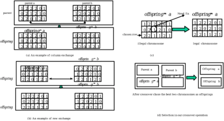
(13) M. selection probability p rwsci is defined as below:. p rwsci = M. ( ). f M ci. ∑ f (M. pop _ size j =1. cj. ). It is obvious that if a chromosome has higher fitness value, then its selection probability is higher. After the selection probability of each chromosome is known, a random number between 0 and 1 is generated for each chromosome. We select the chromosome where the random value falls on and we reproduce this chromosome. We finish this step after pop_size chromosomes are reproduced. 4.6 Perform crossover operation on the selected chromosomes In crossover, we select a pair of chromosomes and do crossover operation on them to exchange information between them. In crossover, a crossover rate p c is first given (the method to determine a proper value of p c will be discussed in detail in Section 5). For each chromosome, a random number between 0 and 1 is generated. If the random number is less than the given crossover rate p c , the chromosome will be marked to indicate that crossover will be executed with it. When all the chromosomes have finished the mark operation, we will in sequence select a marked chromosome and the next marked one to do crossover. Our proposed crossover operation consists of three kinds of actions: column exchange, row exchange, and selection. In column exchange, the two chromosomes will exchange one of their columns. The columns to be exchanged are determined randomly. Figure 4 (a) shows an example of column exchange. Similarly, in row exchange, the two chromosomes will exchange one of their rows. The rows to be exchanged are also determined randomly. Figure 4 (b) shows an example of row exchange. However, the row exchange may generate some errors, which will lead to an illegal slot schedule matrix (See Figure 4(c)). An error happens if there exist consecutive entries with label “1” in the same column. Therefore, each time a row exchange is finished, we must 13.
(14) examine the resulted chromosome to detect if there exist such errors. We will fix such an error by changing the values of entries in the non-selected rows from “1” to “0”. After column exchange and row exchange, two new chromosomes will be generated. Among the four chromosomes (consisting of the two parent chromosomes and the two new chromosomes), we will select the two chromosomes with the higher fitness values as the offspring of the crossover operation and put them into the next generation (see Figure 4(d)). 4.7 Perform mutation operation on the selected genes The purpose of mutation is to generate a variety of chromosomes to avoid the local optimal solution. Given a mutation rate p m (which is decided by simulations). A random number between 0 and 1 is generated for each gene (i.e., each entry) labeled as “0”. If the random number is less than p m , then the corresponding gene will do a mutation, i.e., the value of the entry will be changed into “1”. Like row exchange, mutation may also generate the same errors. Therefore, each time a mutation is executed, we need to do some examinatio ns. To be more specific, we must check both the upper and down adjacent entries of each mutated entry. If they are labeled as 1, then they must be changed 0 to obtain a legal slot schedule matrix (see Figure 5). 5. Computer simulations 5.1. Parameter selection Like other GAs, the performance of our proposed genetic algorithm heavily depends on four important parameters: the number of generations (g), population size (pop_size), crossover rate ( p c ), and mutation rate ( p m ). We will use computer simulations to determine a set of proper values for the four parameters such that our GA may yield the best performance. In our computer simulations, we assume that the length of path is five hops and a frame has sixteen time slots. 14.
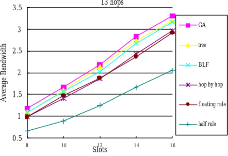
(15) The input of our GA: the free time slots of each node, is generated randomly. Each of the simulation results is obtained through 100 times of simulations. Let us first consider the influence of the number of generations on the finding bandwidth. To determine a best value for p, crossover rate p c is set to 0.1 and mutation rate p m is set to 0.07. Three different values for population sizes pop_size, 100, 75, and 50, are considered. Figure 6 shows the impact of the number of generations g upon the yielded bandwidth. It can be observed that there is almost no any increase in the bandwidth after the number of generations has reached 175. Therefore, we will take 175 as the number of generations in our computer simulations. Next, we will observe the influence of population size pop_size on the yielded bandwidth. Figure 7 shows the results when the number of generation is equal to 175, crossover rate is 0.1, and mutation rate 0.07. From the curve in Figure 7, we can conclude that it cannot lead an apparent increase in the found bandwith to set pop_size to a value larger 100. Under the assumption that the number of generations is, population size is 100, and mutation rate is 0.07, Figure 8 shows the effects of different crossover rates on the bandwidth calculated by our proposed GA. It seems that there exists no any value that is absolutely superior to others. 0.1 is a feasible but not the only choice for crossover rate. Finally, Figure 9 shows the effects of different mutation rates on the bandwidth produced by our proposed GA as the number of generations is 175, population size is 100, and crossover rate is 0.01. From Figure 4.28, we can observe that setting mutation rate to any value between 0.05 and 0.07 performs always well. 5.2 Comparisons between different heuristic algorithms Based on the above discussion on selecting proper values for those four important parameters, in the following, we will examine the efficiency of our GA through computer simulations. Our comparisons will be made among five bandwidth calculation heuristic algorithms. These five heuristic algorithms are the half rule [10] , the floating rule [10], 15.
(16) the hop by hop method [16] , the bottleneck link first algorithm BLF [14], and the tree algorithm [5]. We will evaluate the bandwidth and execution time of each of the six algorithms. In the simulations below, we consider different path lengths and frame sizes. The path length will be increased from 5 hops to 13 hops by a step of 4 hops. The number of slots in a frame will conducted from 8 to 16 by a step of 2. The input to our GA is a common free slot matrix which will be generated randomly. The simulation results of various combinations of path lengths and frame sizes are shown in Figure 10 until Figure 12. It is obvious that the bandwidth generated by our proposed GA is larger than other algorithms. Although both BLF and the tree algorithm consider the whole path in a centralized manner, the tree algorithm has a better performance than BLF. The performance of the hop-by-hop method and the floating rule are almost the same. The half rule performs worse.. 6. Conclusions Unlike in a wired network, where the available bandwidth of a route is simply the minimum bandwidth of the links along the route, the calculation of the available bandwidth of a route in a mobile ad hoc network has been proved to be NP-complete. Based on the principle of genetic algorithms, in this paper, we have designed an efficient heuristic algorithm, which executed in a centralized manner, to solve the bandwidth calculation problem in the CDMA-over-TDMA channel model. Extensive computer simulations have been performed to compare the performance of our proposed GA method and that of other existing heuristic algorithms: the half rule, the floating rule, the hop-by-hop method, the bottleneck link first algorithm, and the tree algorithm. Simulation results verify that our GA can produce larger bandwidth than others.. Reference [1] N. Banerjee and S. K. Das, “MODeRN: multicast on-demand QoS-based routing in wireless networks,” VTC 2001, Vol. 3, pp. 2167-2171, MAY 2001. [2] N. Banerjee and S. K. Das, “Fast determination of QoS-based multicast routes in wireless networks using genetic algorithm,” ICC 2001, Vol. 8, pp. 2588-2592, June 2001. [3] J. Broch, D. B. Johnson, and D. A. Maltz, “The dynamic source routing protocol for mobile ad hoc networks,” Internet-Draft, draft-ietf-manet-dsr-01.txt, Dec. 1998. 16.
(17) [4] S. Chen and K. Nahrstedt, “Distributed quality-of-service routing in ad hoc networks,” IEEE J. Select. Areas Commun., pp. 1488-1505, Aug. 1999. [5] Y. S. Chen, Y. C. Tseng, J. P. Sheu, and P. H. Kuo, “An on-demand, link-state, multi-path QoS routing in a wireless mobile ad hoc network,” to appear in European Wireless, 2002. [6] C. Ferguson, “Routing in a wireless mobile CDMA radio environment,” Ph.D. thesis, University of California , computer science department, Los Angle, 1996. [7] C. M. Fonseca and P. J. Fleming, “Genetic algorithm for multiobjective optimization: formulation, discussion and generalization,” Proc. of the Fifth International Conference on Genetic Algorithms, pp. 416-423, 1993. [8] M. Gen and R. Cheng “Genetic algorithms and engineering design,” JOHN WILEY & SONS, ISBN:0-471-12741-8, 1996. [9] R. H. Hwang, W. Y. Do, and S. C. Yang, “Multicast routing based on genetic algorithms,” Journal of Information Science and Engineering, vol. 16, pp. 885-901, 2000. [10] Y. C. Hsu; T. C. Tsai; and Y. D. Lin, “QoS routing in multihop packet radio environment,” Proc. of IEEE ISCC '98, pp. 582-586, July 1998. [11] C. R. Lin, “On-demand QoS routing in multihop mobile networks,” Proc. of IEEE INFOCOM 2001, vol. 3, pp. 1735-1744, April. 2001. [12] C. R. Lin, “Admission control in time-slotted multihop mobile networks,” IEEE J. Select. Areas Commun., pp. 1974-1983, Oct. 2001. [13] Y. Leung, G. Li, and Z. B. Xu, “A genetic algorithm for the multiple destination routing problems,” IEEE Trans. Evolutionary computation, vol. 2, pp. 150-161, NOV. 1998. [14] H. C. Lin and P. C. Fung, “Finding available bandwidth in multihop mobile wireless networks,” Proc. of IEEE VTC 2000, vol. 2, pp. 912-916, May. 2000. [15] C. R. Lin and M. Gerla, “Asynchronous multimedia multihop wireless networks,” Proc. of IEEE INFCOM’97, vol. 1, pp. 118-125, Aprial 1997. [16] C. R. Lin and J. S. Liu , “QoS routing in ad hoc wireless networks,” IEEE J. Select. Areas Commun., pp. 1426-1438, Aug. 1999. [17] W. H. Liao, Y. C. Tseng, and K. P. Shih, “A TDMA-based bandwidth reservation protocol for QoS routing in a wireless mobile ad hoc network,” to appear in IEEE ICC, 2002. [18] W. H. Liao, Y. C. Tseng, S. L. Wang, and J. P. Sheu, “A Multi-Path QoS Routing Protocol in a Wireless Mobile Ad Hoc Network,” IEEE Int'l Conf. on Networking (ICN), 2001. [19] V. D. Parh and M. S. Corson, “Temporally-Ordered Routing Algorithm (TORA) version 1 functional specification,” Internet-Draft, draft-ietf-manet-tora-spec- 03.txt, Nov. 2000. [20] C. E. Perkins and E. M. Royer, “Ad-hoc on demand distance vector routing,” Proc. of IEEE WMCSA’99, pp. 90-100, Feb. 1999. [21] A. Roy, N. Banerjee, and S. K. Das, “An efficient multi-objective QoS-routing algorithm for wireless multicasting,” IEEE VTC 2002, vol. 3, pp. 1160-1164, May, 2002.. 17.
(18) l 12. l23. {1,5,6}. v1. v2. l34. {1,3,5,6}. {3,4,6}. v3. v1 v2 v3 v4. v4. (a) Common free slots 1 2 3 4 5 6 A. A. A. A. A. F. F F F F. F F. F F F. parent a. A. A A. parent b. 1 2 2 2 0 1 0 2 1 2 1 0 2 2 0 1 2 1. parent. F. offsprin g ′ 1 2 2 2 0 0 2 0 2 1 2 2 1 1 2. A offspring. Aà available. A. A. A. A. A. 0 2 2 2 0 1 1 2 0 2 1 0 2 2 1 1 2 1. offsprin g ′′ a. a 1 0 1. chosen row. 0 2 2 2 0 1 1 2 1 2 1 0 2 2 0 1 2 1. R U. R U R. U. R. R. U R. m1 = 6. 1 2. 2 2. 0 1. 0 2. 1 2. 1 0. 2 2. 0 1. 2 1. 1 2 2 2 0 1 0 2 0 2 1 0 2 2 1 1 2 1. illegal chromosome. legal chromosome. (c). offsprin g ′ b. (c) Common free slot matrix Rà reservable Uà unreservable. offspring. àunavailable (d) A {3*6} slot schedule matrix 0àunreservable 1à reservable 2àunavailable (e) A chromosome. offsprin g ′′ a. Need fix. 1 2 2 2 0 1 0 2 1 2 1 0 2 2 1 1 2 1. offsprin g ′ b. àunavailable. A. m1 = 6. m2 = 3. F. ( a) An example of column exchange. A A. m2 = 3. A. F F F. F. (b) Common free slot vector. m1 = 6 m2 = 3. A. F F. 1 2 3 4 5 6. 1 2 3 4 5 6 A. 1 2 3 4 5 6. offspring. 1offsprin 2 2 2g ′0a 1 0 2 1 2 1 0 2 2 0 1 2 1. 0 2 2 2 0 1 1 2 0 2 1 0 2 2 1 1 2 1. 1 offsprin 2 2 2 g0′ 1a 0 2 1 2 1 0 2 2 1 1 2 1. 0 2 2 2 0 1 1 2 0 2 1 0 2 2 0 1 2 1. Parent a. Parent b. Offspring. a. Offspring. b. offsprin g ′′ b offsprin g ′′ a. offsprin g ′′ b. After crossover chose the best two chromosomes as o f f s p r i n g s. (d) Selection in our crossover operation ( b) An example of row exchange. depicted as a {3*6} matrix. Figure 4. The crossover operation in our GA consisting of Figure 1. Notations column exchange, row exc hange, and selection START Input data( the common free slot matrix of a given path) Generate an initial population of chromosomes from input data. Evaluate chromosome in the initial population. Before mutation. Termination judgment Reproduction. Solution Is it the initial population. no. ?. y e s. replacement. 1 0 2. 2 2 2. 2. 2. 0. 1 0. 2 1. 1 2. After mutation 1 0 1. 1 0. 2 2. 2. 2. 2 1 0. 2 2 1. 0 1 2. After fix 1 1. 1 0. 2 2. 1. 2. 2. 2 1 0. 2 2 1. 0 1 2. 0 1 0. roulette wheel selection method. Need fix. Mutation element. Perform crossover operation on the selected chromosome. After fix. Perform mutation operation on the selected chromosome. Evaluation. Figure 2. The flowchart of pur proposed genetic algorithm. Figure 5. The mutation operation in our GA. Parent chromosomes. The effect of generation number. (pop_size). The next generation (pop_size) Offspring chromosomes generated from a series of genetic operations (pop_size). 5.1 5.05. (a) The replacement action in our reproduction. Mc p o p_ rws. P. size. Mc Prws. 1. 5 Average Bandwidth. The top 50% chromosomes. pop_size=100. 4.95 4.9. pop_size=75. 4.85 4.8. Mc Prws. 2. … Mc Prws. pop_size=50. 4.75 4.7. 3. 25. 50. 75. 100 125 150 175. 200 225. 250 300 350. 400 450 500. Generation. (b) The roulette wheel selection method. Figure 3. The reproduction operation in our GA. Figure 6. The effect of generation number on our proposed GA. 18.
(19) The effect of population size. 5 Hops. 4.5 4 Average Bandwidth. Average Bandwidth. 5.15 5.1 5.05 5 4.95 4.9 4.85 25. 50. 75. 100. 125. 150. 2. hop by hop. 1.5. floating rule half rule 8. 10. 12. Slots. 14. 16. Figure 10. Average bandwidth for path length=5 Hops. The effect of crossover rate. 9 hops. 4. GA. 3.5 Average Bandwidth. 5.1 Average Bandwidth. BLF. 2.5. 0.5. Figure 7. The effect of population size on our proposed GA. 5.05 5 4.95 4.9 4.85. tree. 3 2.5. BLF. 2. hop by hop. 1.5. floating rule. 1 0.1. 0.2. 0.3. 0.4. 0.5. 0.6. 0.7. 0.8. 0.9. half rule. 0.5. Crossover rate. 8. Figure 8. The effect of crossover rate on our proposed GA. 10. 12. Slots. 14. 16. Figure 11. Average bandwidth for path length=9 hops. The effect of mutation rate. 13 hops. 3.5. 5.5. GA. 3. 5. Average Bandwidth. Average bandwidth. tree. 3. 1. Population size. 4.5 4 3.5 3. GA. 3.5. 0.01 0.02 0.03. 0.04 0.05. 0.06 0.07 0.08. 0.09. 0.1. 0.2. 0.3. 0.4. 0.5. 0.6. 0.7. 0.8. 0.9. tree. 2.5. BLF. 2 hop by hop. 1.5 floating rule. 1 half rule. Mutation rate 0.5 8. 10. 12. Slots. 14. 16. Figure 9. The effect of mutation rate on our proposed GA Figure 12. Average bandwidth for path length=13 hops. 19.
(20)
數據
相關文件
Various learning activities such as exp eriments, discussions, building models, searching and presenting information, debates, decision making exercises and project work can help
These learning experiences will form a solid foundation on which students communicate ideas and make informed judgements, develop further in the field of physics, science
The A-Level Biology Curriculum aims to provide learning experiences through which students will acquire or develop the necessary biological knowledge and
The temperature angular power spectrum of the primary CMB from Planck, showing a precise measurement of seven acoustic peaks, that are well fit by a simple six-parameter
Like the proximal point algorithm using D-function [5, 8], we under some mild assumptions es- tablish the global convergence of the algorithm expressed in terms of function values,
Shih, “On Demand QoS Multicast Routing Protocol for Mobile Ad Hoc Networks”, Special Session on Graph Theory and Applications, The 9th International Conference on Computer Science
Microphone and 600 ohm line conduits shall be mechanically and electrically connected to receptacle boxes and electrically grounded to the audio system ground point.. Lines in
“Ad-Hoc On Demand Distance Vector Routing”, Proceedings of the IEEE Workshop on Mobile Computing Systems and Applications (WMCSA), pages 90-100, 1999.. “Ad-Hoc On Demand
