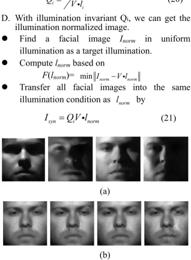
Illumination Normalization of Facial Images for
Face Recognition
Shao-Yung Huang and Chung-Lin Huang
Electrical Engineering Department, National Tsing-Hua University Hsin-Chu, Taiwan, ROC
e-mail: [email protected], [email protected]
However, to solve the illumination problem for face recognition, most of the existing methods either use extracted small-scale features and discard large-scale features, or perform normalization on the whole image. In the latter case, the small-scale features may be distorted, whereas in the former case, large-scale features of facial image are not utilized. Different from previous research, Xie et.al [7] proposed a new framework which uses not only invariant small-scale feature but also considers illumination normalized large-scale feature to reconstruct an illumination normalized facial image for face recognition.
Abstract―In the paper, we focus on how to reconstruct
the illumination normalized facial image which can be used to improve the face recognition. Here, we employ a framework to process large-scale and small-scale features image independently. In this frame work, first, we decompose the facial image into a large-scale feature image and a small-scale feature image. Second, once a facial image is decomposed into a large-scale feature image and a small-scale feature image, normalization is then mainly performed on the large-scale feature image. Then, a smooth operator is applied on the small-scale feature image. Finally, we combine the large- and small- scale feature images to generate an illumination normalized facial image. We test our method using Yale B & Extend Yale B database. The experimental result shows that image processed by our method not only has better visual quality, but also can be used to improve the performance of face recognition.
Since most of the existing methods aim at either small-scale features or the whole facial image, it is hard to get good recognition performance and generate normalized facial image. In this paper, we focus on how to reconstruct the illumination normalized facial image, to improve recognition result and generate good visual quality.
Index Terms― facial image illumination normalization,
face recognition.
I. INTRODUCTION
Face recognition technologies have been widely applied in the areas of intelligent surveillance, identity authentication, human-computer interaction and digital amusement. However, there are many limitations in deploying the face recognition for practical use such as pose, view point and illumination variations. It has been observed that the influence of illumination variations for face verification is more significant than the other effect [1]. Most existing methods for face recognition such as PCA [2], ICA [3] LDA [5] based methods are sensitive to illumination variations [4]. Therefore, Illumination normalization is a major issue in the face recognition process.
To reach our goal, we employ a framework to process large-scale and small-scale features image independently. In this frame work, first, we decompose the facial image into a large-scale feature image and a small-scale feature image. Second, once a facial image is decomposed into a large-scale feature image and a small-scale feature image, normalization is then mainly performed on the large-scale feature image. Then a smooth operator is applied on the small-scale feature image. Finally, we combine the large- and small- scale feature images to generate an illumination normalized facial image.
There are many different illumination variations in the real facial images. If we can normalize the images to a uniform illumination, then we may increase the accuracy of face recognition. The illumination normalization has become a critical issue for facial image processing, and many well-known algorithms have been developed to take this problem.
II. IMAGE DECOMPOSITION USING ADAPTIVE SMOOTHING 2 1 ( , ) ( , ) ( , ) ( , ) ( , ) ( , ) . . ( ) ( )
norm filt norm
filt norm I x y x y S x y I x y x y S x y s t T S T S ρ ρ ρ ρ = ⎧ = ⎪ = ⎨ ⎪ = ⎩ (3) In this section, we describe the system
overview and explain how we can decompose a facial image into small-scale feature and large-scale feature image. Based on the Lambertian model, a
facial image I can be represented by decomposition, smoothing on small-scale feature It consists of four steps, namely facial image image (T2), illumination normalization on large-scale feature image (T1) and reconstruction of normalized images.
I = r nT il = R ⊗ L (1)
where r is the albedo of face, n is the surface normal of face, • is the dot product, l is the illumination and ⊗ is the pointwise product. R indicates the reflectance image and L represents the illumination image. Many proposed researches try to extract the reflectance image for face recognition. Unfortunately, estimating R from I is an ill-posed problem. To solve this problem, Chen et al. [6] proposed a practical methodology. R denotes as the albedo of large-scale skin areas and background. Then, based on Eq. (1), we have the following
A. Algorithm Overview
Doing illumination normalization, first we decompose a facial image into a small-scale image and a large-scale image as shown in Eq.(2). In this paper, we employ recently developed adaptive smoothing [8] for image decomposition. Adaptive smoothing is a weighted smoothing which is based on both iterative convolution and two discontinuity measures. Further more, we also employ some new concepts, which are designed to be suitable especially for facial image. One is the new conduction function for adaptive weighting, and the other is the smoothing constraint for more accurate description of real environments. Compared with
the existing method, adaptive smoothing has the capabilities of edge-preserving and small-scale features extracting. ( , ) ( , ) ( , ) ( ( , ) / ( , ))( ( , ) ( , )) ( , ) ( , ) l l I x y R x y L x y R x y R x y R x y L x y x y S x y ρ = = = (2)
In this framework, the former term ρ(x, y) contains only the smaller intrinsic structure of a facial image, and the later term S(x, y) contains not only the extrinsic illumination and shadows casted by bigger objects, but also the large intrinsic facial structure. In this paper, we regard ρ(x, y) as the small-scale feature image and S(x, y) as the large-scale feature image.
Fig.2. Image decomposition overview. Since, the influence of illumination variation on
large-scale features of a facial image, it is essential to maintain illumination-invariant small-scale features during illumination normalization. From Eq.(2), we notice that an image can be decomposed into a small-scale feature image and a large-scale feature image. Therefore, we do illumination normalization on large-scale feature images; meanwhile keep the small-scale intrinsic facial features in ρ unchanged. The illumination normalization on large-scale feature image needs some necessary processing on ρ, which is independent of the one on S. From Eq(2), we propose a framework for illumination normalization described as follows:
B. Illumination Estimation
The key idea of adaptive smoothing is to convolve the input image iteratively using a 3 × 3 averaging mask whose coefficients repersent the discontinuity level of the input image at each point. Since we estimate illumination L as a smoothed version of input image I, we set the initial value of the estimated illumination (i.e., ) be the same as I(x, y). Therefore, the estimated illumination is represented as at the (t+1)th iteration which is given by
(0)( , ) L x y ( 1)t ( , L + x y) 1 1 ( 1) ( ) ( ) ( ) 1 1 1 ( , ) ( , ) ( , ) t t t t i j L x y L x i y j w x i y j N + =− =− =
∑∑
+ + + + (4)where 1 1 ( ) ( ) 1 1 ( , t t ) N w x i y j − − =
∑∑
+ + ,w x y( )t( , )=g d x y( ( )t ( , )),N(t) represents normalizing factor. A conduction function g is a nonnegative monotonically decreasing function, i.e., g(0)=1 and
as increase.
represents the amount of discontinuity at each pixel (x, y). For more efficient setting of , we will combine two discontinuity measures[9].
( )t →0 ( )t ( )t ( )t ( ( , )) g d x y d ( , )x y d ( , )x y ( , ) w x y C. Discontinuity Measures
We use two measurements of discontinuities, spatial gradient and local in-homogeneity, to determine the level of discontinuity at each pixel. a) Spatial Gradient
The spatial gradient is a common local discontinuity measure. Therefore, we define the spatial gradient of an image I(x, y) at pixel (x, y) as the first partial derivatives of its image intensity function with respect to x and y as.
( , ) ( , ) ( , ) [ x, y] [ , ] I x y I x y I x y G G x y ∂ ∂ ∇ = = ∂ ∂ (5)
The magnitude of the gradient vector in (5), ( , ) 2 2
x y
I x y G G
∇ = + (6) b) Local In-homogeneity
In addition to spatial gradient, Chen [9] proposed a method by using in-homogeneity as another measure of discontinuity. This measure is very efficient, however, it is very time consuming. Therefore, we employ another measure that is just the average of local intensity differences for each pixel (x, y) in the facial image. This measure is called local in-homogeneity, which provides us the level of uniformity for all the pixels in the small neighborhood of current pixel. If local in-homogeneity at pixel (x, y) is large, then we find the discontinuity occurring at pixel (x, y). The average of local intensity differences at pixel (x, y) is described by
τ( , )x y = ( , )m n∈Ω I x y( , )−I m n( , ) Ω
∑∑
(7)
where Ω is a convolution region, and (m, n) indicates the locations of the surrounding pixels.
Then, we normalize the average τ(x, y) at each pixel as min max min ( , ) ˆ( , )x y τ x y τ τ τ τ − = − (8) where τmax and τmin are the maximal and minimal
values of τ across the entire facial image. We apply a nonlinear transformation to emphasize the higher values which are more likely corresponding to cast shadow as ( , ) sin( ˆ( , )),0 ( , ) 1 2 x y π x y x y τ = τ ≤τ ≤ ( , ) ( ( , ), ) (9) Although we calculated this measure of its nearest neighborhood only, the propagation effect of local in-homogeneity many continue by an iterative convolution.
D. Conduction Function and Smoothing Constraint
With two discontinuity measures, we define proper conduction function for our discontinuity measures. Hence, g is nonnegative monotonically decreasing function, because a large weight should be assigned to a pixel that involves low discontinuity. A nonnegative monotonically decreasing function g is employed to both spatial gradient and local in-homogeneity as follows.
α x y =g τ x y h (10) β( , )x y =g(∇I x y S( , ) , ) (11) where h(0<h<1) and S(S>0) are used to determine the level of discontinuities which must be preserved. There are many possible selections of g. Chen [9] has proposed
Hence, we employ a new form of g without edge sharpening effect as 1 ( , ) 1 g z K z K = + (12) The values of S and h (in Eq. (10) and (11)) are e
d termined experimentally. Here, we let S = 1 and h = 0.1 for facial image normalization. Now, we can determine the corresponding weights of the convolution maskw( )t ( , )x y by using α and β as
( )t ( , ) ( , ),
w x y =α( , )x y β x y ∀ (13) t E. Algorithm
e set input image as an illuminated Initialization: w
z Computation of the adaptive smoothing weight as ( , )w x y =α( , ) ( , ),x y β x y ∀ t
z Iteration until t=T, Perform iterative convolution to update L x y as ( )t ( , ) 1 1 ( 1) ( ) ( ( ) 1 1 ( , ) ) t t t t i j L x y L x i y j w N + =− =− =
∑∑
+ + )(x i y j+ , + ) where ( ) 1 1 ( ) 1 1 ( , ) t t i j 1 ( , N w x i y j =− =− =∑ ∑
+ +z Get small-scale features as
( )( , ) ( , ) ( , ) / T R x y =I x y L x y (a) (b) (c)
Fig.3. (a) th original facial image from Yale B face database, (b) the large-s feature images, (c) the small-scale feature imag
FEATURES
illuminati mage by
using Gen 1] which
is
e-scale feature image S(x, y) may also contain the larger intrinsic
fa
we develop ge-scale feature roperty from the ex be hich is t, which is e
cial structures which are illumination invariant. Therefore, different from most illumination normalization algorithm, we apply the illumination-normalization on the large-scale feature images. To remove the illumination effect in large-scale feature images, an effective illumination normalization processing is employed.
A. Generalized Quotient image
Each image contains intrinsic information as will as extrinsic information. In this section,
a representation of an input lar image by separating the intrinsic p
trinsic one. Then, we can eliminate the extrinsic property which contains illumination-variation. 1) Intrinsic and Extrinsic Factorization
A typical Lambertian model can be factorized into two parts. A large-scale feature image can decomposed into the intrinsic part, w illumination invariant, and the extrinsic par illumination variant, described as follow:
( , )S x y = • (14) F L where F donates the intrinsic part in large-scale feature image, and L is the extrinsic part in large- ture image. By separating the two factors, we can recover the extrinsic property. scale fea
cale
es. Fig. 4. General quotient image framework. 2) Illumination Normalization
T wo
main (2)
irst, the extrinsic ated and a
III. ILLUMINATION NORMALIZATION ON
LARGE SCALE he illumination normalization consists of t steps: (1) Illumination estimation Here, we describe how to eliminate the
on effect on large-scale feature i eralized Quotient image [10][1
Illumination effect subtraction. F
factor in large-scale feature image is estim
synthesized image is generated. The synthesized large-scale feature image has the same illumination and 3D shape as the input but different albedo. Then the illumination is normalized by taking the difference between the input and the synthesized images in the logarithms. Since the synthesized image has the same illumination and 3D shape with applied for extracting illumination invariant
representation of the facial image.
Most the extrinsic illumination and shadows cast by bigger objects will appear in the large-scale feature image. However, the larg
the original one, the normalized image is (logρ0 − logρ1), where ρ0 and ρ1 are input and synthesized images.
B. Non-Point Light QI (NPL-QI)
Here, we assume that all the modeled objects have the same 3D shape as the original QI. NPL-QI, of QI from a illumination co
luminated with a light source without shadow.
ages are always ill
extends the illumination estimation single point light source to any type of
nditions, by taking the advantage of the linear relationship between spherical harmonic bases and PCA bases. Instead of explicitly estimating the 3D face shape, we replace the spherical harmonic bases with their linear transformed version, PCA bases. NPL-QI has the same invariant form, albedo ratio of two faces, as the original QI.
1) Analysis
The original QI method works only under the assumption of facial image il
single point
Nevertheless, the common facial im
uminated by non-point light sources in which shadow may exist unless the face is illuminated only by frontal lighting. According to [12~15] spherical harmonic representation, facial image I can be represented by
I =ρH oi (15) where H =[ , ,h h h1 2 3,..., ]hn is the spher harmonic bases and o is the harmonic light. Based on their research, the first 9 h
ical armonic bases can be used to describe the image of diffuse object, such
an face. as hum
Fig. 5. The first nine harmonic images for a model of a face in [15].
not suitable for general According to [13], there is a linear relationship be
Because these bases must be calculated with known 3D geometry, the application range of this
representation is case.
tween PCA eigenvectors and spherical harmonic bases as
U =BT (16)
Where U =[ , , ,..., ]u u u1 2 3 un is the eigenvector matrix of a facial image under all illumination conditions, B represents
ba
ca d to tr
the spherical harmonic ses, and T is n-by-n transformation matrix which n be use rmonic light o into l. Therefore, the Eq.15 can be described as ansform the ha
I =B o U li = i (17) where l T o= −1 .
Since we have densely samp
in Yale B [16], we can obtain U, which is a well a -transferred spherical
ic from PCA
w
led images, such as approxim
harmon bases Replacing these basested for linear.
ith three images in QI, we have the NPL-QI as
y i i y i y y a a i i i h o I Q h o U l ρ ρ ρ ρ = =
∑
=∑
In some extremely illuminated facial images, there are obvious cast shadows. Therefore, th
9 eigenvectors can not carried over
energy. Obviously, more eigenvectors are needed in th
nd M is the cial images under different lighting
global lighting space.
i (18) e first 95 % image e implementation of this algorithm.
2) Algorithm
A. Let D be an N-by-M matrix, where N is the number of pixels of facial image a
number of fa condition.
z We choose the facial images of the same person in Face database with the frontal pose but systemically sampled lighting conditions for building
B. Compress these images by Singular Value Decomposition (SVD), and let V = [v1, v2, ..., vk] be the first K eigenvectors of D.
t
z Let D U V= Σ , find the first k eigenvector of D, therefore, Σ becomes Σ v
z Then we have t v
V U V= Σ
C. Compute li in quotient image, then we have the
quotient image Qi for each faci la image Iiin the li,.
database by the ratio of Iiand V •
z Find li with the characteristic
( ) mini i i
F l = I V l− i (19) z Compute Quotient-Image Qi by
i i i I V l = i
e can get the illumination normalized image.
z Fin facia
Q (20) D. With illumination invariant Qi, w
d a l image Inorm in uniform
illumination as a target illumination. z Compute lnorm based on
F(lnorm)= min Inorm− iV lnorm
z Transfer all facial images into the same illumination condition as lnorm by
Isyn =QVi ilnorm (21)
(a)
(b)
Fig. 6. (a) the original large-scale feature image; (b) the normalized large scale feature image.
IV. MIN-FILTERING SMALL SCALE age
T t
part in facial i eature image, ale ill
linear spatial filtering
age area encompassed by the
spots. To
e filter kernel will
ON FEATURE IMAGE A. Light Spot on Small Scale Feature Im
hough, we try to separate illumination-invarian mage as small scale f
some light spots may appear in the small-sc feature image ρ under some challenging
umination condition. Because some influence caused by extreme illumination might falls on some small-scale feature of face such as the corner of eye, nose or mouse. Although these light spots might not have influence on the result of face recognition, it would have negative effect on the visual of the reconstructed image. Therefore, we have to do some special filtering on small-scale feature image, to reduce these light spots.
B. Threshold Min-filtering on Small Scale Feature Image
Minimum filter is a non
whose response is based on ordering the pixels
contained in the im
filter, and replacing the value of the center pixel with the pixel determined by the ranking result. The best-known example in this category is the median filter, which replaces the value of a pixel by the median of the gray levels in the neighborhood of that pixel. They provide excellent noise-reduction capabilities, with considerably less blurring than linear smoothing filters of similar size.
Most noise in our small-scale feature image appears as light spots. Therefore, we choose minimum filter to eliminate these light
reduce the influence on whole small-scale feature image, we employ the threshold minimum-filtering on small-scale feature images.
Suppose (x, y) is the center point of our convolution region. Then, the threshold minimum filtering performs as follows. Th
convolute only if small-scale feature images ρ(x, y) ≥θ , where θ is an empirical threshold. A 3× 3 mask is applied in our threshold minimum filtering. A small-scale feature image is convolved twice. Some examples of the filtering result is illustrated as follow.
(a)
(b)
Fig.7. (a) Original small-scale feature images after image decomposition, (b) The small-scale feature images after applying m ring.
, ge, which m
in-filte
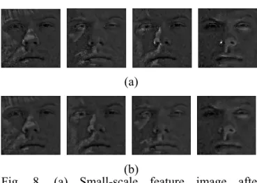
C. Smoothing on Small-Scale feature images After applying min-filtering on small-scale facial images, most light spots are eliminated. However there are still some noise on our facial ima
ight caused by some extreme illumination conditions. To improve visual quality distorted by noise, we do average filtering on small-scale feature image. The average filter can reduce noise, however; too many times of average filtering will blur the small-scale feature. Therefore, we apply the average filtering on small-scale feature image only once. So that we can reduce noise and keep
most small-scale feature at the same time.
(a)
(b)
Fig. 8. (a) Small-scale feature image after min-filterin , (b) Small-scale featur image aft average filtering.
scale feature image are obtain tion facial lized facial im
g e er
D. Reconstructing normalized image
After a normalized large-scale feature image and
the filtered small- ed,
we can reconstruct a uniform-illumina image. Similar to Eq. (3), the norma
age is finally reconstructed by combination of the normalized large-scale feature image Snorm and
the filtered small-scale feature image ρfilt , as
follow.
( , ) ( , ) ( , )
norm filt norm
I x y =
ρ
x y s x y (22)Using the illumination normalization result in previous section and the filtered small-scale feature image, we can reconstruct our final res
simple reconstruction results are shown in Fig. 9.
(a)
(b)
(c)
Fig.9. (a) The normalized large-scale feature images, (b) The filtered small-scale feature image, (c) The reconstruction result from large-sc le
feature and small-scale f re image.
performing
illuminati eature
images outperform age;
(2
s are evaluated by using
s of base are captured under rom 9 different poses of vi
ult. Several
eatu
V. EXPERIMENTAL RESULTS
Here, some experiments are conducted to verify the following two assumptions: (1)
on normalization on large-scale f s that on the whole facial im ) large-scale features discarded in other algorithms are also useful for face recognition and should not be ignored.
To evaluate the visual quality of the reconstructed images, the Yale B and Extend Yale B databases are selected in our experiment. The performances of algorithm
a SVD-Based projection face recognition [17]. A. Yale face B Database
For evaluation our method, Yale B [16], Extend Yale B databases are selected. The facial image each person in Yale B data
64 different illuminations f
ews. We select the frontal facial images in Yale B database for our experiments; therefore, there are 640 images from Yale B. Subjects in Yale B database are shown in Fig.10.
Fig. 10. Ten facial images in Yale B database. More than Yale B database, extended Yale B is also selected for evaluation. In the Extended Yale B
dat d under 64 illum as ethods. In our e fil
abase, there are 28 human subjects capture inations which is the same condition Yale B. In our experiment, only the frontal facial images from these two databases are selected. All images are resized to 150*150.
B. Visual Quality of the Reconstructed Images In this section, we compare the results of our illumination normalization m
a
framework, illumination normalization is applied only on the large-scale feature images, and som
tering is performed on small-scale features. Therefore, we can protect the most small-scale features from being distorted by illumination
normalization. To compare the visual quality between our method and other methods, we apply NPL-QI and LOG-DCT methods on the whole facial image and compare with the results of our method. We also show the visual result of our method and the result in [7].
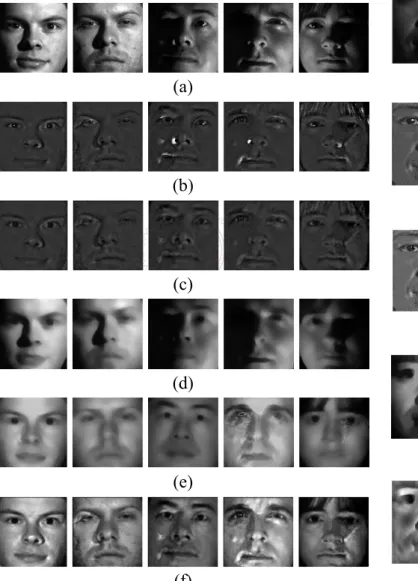
Here, we show image decomposition results in details as shown in Fig.11. Our method preserves the intrinsic facial structures in small-scale feature images well, and most illumination variations are kept in large-scale feature images. Therefore, the illumination in large-scale feature images can be better estimated in our framework.
(a) (b) (c) (d) (e) (f)
Fig. 11. (a) the original facial images, (b) the small-scale feature images, (c) the filtered small-scale feature im , (d) the large-scale feature images, (e) th normalized large-scale
et al. proposed a m
ages e
feature images, (f) the reconstruct facial images. In Fig. 12, we show the image decomposition results, i.e., small-scale and large-scale feature
images and the illumination normalization. Xie. ethod using LTV model [7] to decompose facial image to small- and large- scale features image, and perform illumination normalization on large-scale feature images, and smoothing on small-scale feature images. Finally, a normalized large-scale feature image and a filtered small-scale feature image are used to reconstruct an illumination-normalized facial image. In [7], two methods are applied to do illumination normalization on large-scale feature image, one is LOG-DCT [18], and the other is NPL-QI.
(a) (b) (c) (d) (e) (f)
(g)
(h)
Fig. 12. Illustration of the corresponding processing
lts, we also pe
ages by
Method Recognition Rate (%) on large- and small- scale feature images (a) the original images, (b) the small-scale feature image ρ, (c) the filtered ρ, (d) the large-scale feature image S, (e) the S normalized by LOG-DCT, (f) the S normalized by NPL-QI., (g) the images normalized by RLS(LOG-DCT), (h) the images normalized by RLS(NPL-QI).
Besides showing the visual resu
rform face recognition on normalized facial images, which also provide a measurement of the reconstructed facial image quality. We compare the performance of our method with the others by a SVD-Based projection face recognition algorithm [17]. In our experiment, Yale and extend Yale B face database is selected for face recognition. There are 38 different subjects and 64 illumination variations for each subject in Yale and extend Yale B face database. We choose 6 images which are under normal illumination condition as training set, and other images as testing set.
Having tested the reconstructed facial im
using a SVD-Based projection face recognition algorithm [17], we may show that our algorithm can improve recognition result significantly. The recognition rate of other methods is shown in Table 1, in which our method is called "AS(NPL-QI)”. Table 1. Comparison of different illumination normalization methods on “Yale B & Extend Yale B”.
Original 25.8
HE 43.4 NPL-QI 66.1
As described in Table 1, the histogram equal little impr nt for face re
estimation. However, too much sm tures w he illumination no use small-scale n and discard the lar
[19] is reported for co
used for face
LOG-DCT 75.2
AS(NPL-QI) 84.3
ization makes oveme
cognition performance. Because it is only suitable for processing the entire image which is either too dark or too bright. However, in Yale B database, most facial images are dark in some parts of image. Obviously, histogram equalization is not a good solution to illumination variation. The spatial non-uniformity of illumination variation is not taken into consideration in histogram equalization.
In NPL-QI, it is very important to obtain good illumination
all-scale features on the facial image will make it hard to estimate illumination condition correctly. If we cannot estimate illumination correctly, the performance of illumination normalization will be limited. The result of recognition rate shows that there is something to be improved in NPL-QI.
For LOG-DCT, thought recognition rate is significantly improved, the small-scale fea
hich are very important for face recognition will be distorted as low-frequency coefficient truncated. Distorting small-scale features will decrease the performance of face recognition.
As shown in Table 1, our method preserves the small-scale features when t
rmalization is applied on the large-scale feature images only. Therefore, our method has better performance in face recognition.
C. Using Large-Scale Features Most proposed methods only features image for face recognitio
ge-scale features in facial image. Thought small-scale features are very important for face recognition, some larger intrinsic facial structures are also invariant to illumination may be contained in the large-scale features. In this experiment, we show that using large-scale features can improve the performance of face recognition, and they should not be discarded.
To demonstrate the advantage of our framework, the adaptive smoothing
mparison. The setting of the experiments is the same as the one in previous section. For adaptive smoothing, the iteration number is set to be very small (10 in our experiments). The results of our experiment are tabulated in Table 2.
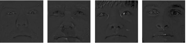
In [19], adaptive smoothing is applied to obtain only small-scale features which are
recognition. Our method performs the illumination normalization on both large- and smoothing on small- scale feature images. Finally a reconstructed image is obtained, which is used for face recognition. In Table 2, we show that our method gives higher recognition rates on “Yale B & Extend Yale B”. It means that the normalized large-scale features can help improving the performance of face recognition.
Fig.13. Small-scale features images from adaptive smoothing.
Fig.14. Rec struct faciaon l images from (NPL-QI). Table 2. Comparisons between using & discarding large-scale features on “Yale B & Extend Yale B”.
Method Recognition Rate (%) Adaptive Smoothing 74.8
AS(NPL-QI) 84.3
VI. CONCLUSIONS
In this paper n algo
for illumination no age.
Ra
fe
REFERENCE
[1] Y. Adini, Y. Ullman. “Face
Recognition: f Compensating
Neurosci, 3, Recognition by Idenependent
ace
vs. Fisherfaces:
, “Total Variation Models for Variable
n Normalization on
estimation/normalization based on
on
e-rendering and , we have introduced a
rmalization on facial imrithm
adaptive smoothing for robust face recognition,” IEEE ICIP, pp 149-152, 2007.
[9] K. Chen, “Adaptive smoothing via contextual
and local discontinuities,” IEEE Trans. ther than doing illumination normalization on
the whole facial image or discarding the large-scale features, the proposed framework can protect small-scale features by doing illumination normalization on large-scale features and smoothing on small-scale features independently.
We may try different method to decompose facial image into small-scale and large-scale
[1
atures. Thought adaptive smoothing has good protection for large discontinuities, there are some discontinuities which cannot be reduced by simple filtering on the small-scale features image. Therefore, if we can find a good method that decomposes facial image without bringing any discontinuities into small-scale feature image, it may help us improve the reconstruction result in
this framework.
Moses and S. The Problem o
for Changes in Illumination Direction,” IEEE TPAMI, 19(7), pp.721-732, 1997.
[2] M.Turk and A.Pentland. “Eigenfaces for
Recognition,” Journal of Cognitive pp.71–86, 1991.
[3] M. S. Bartlett, J. R. Movellan and T. J.
“Sejnowski. Face
Component Analysis,” IEEE Transactions on Neural Networks, 13(6):1450-1464, 2002.
[4] X. D. Xie and K. M. Lam,” An Efficient
Illumination Normalization Method for F Recognition,” Pattern Recognition Letters, 27(6), pp. 609-617, 2006.
[5] P. N. Belhumeur, J. P. Hespanha, and D. J.
Kriegman,“ Eigenfaces
Recognition Using Class Specific Linear Projection,” IEEE TPAMI, 19(7), pp. 711–720, 1997.
[6] T. Chen, X. S. Zhou, D. Comaniciu and T.S.
Huang
Lighting Face Recognition,” TPAMI, 28(9), pp.1519-1524, 2006.
[7] X. Xie1, W.S. Zheng1,3, J. Lai, P. C. Yuen,
“Face Illuminatio
Large and Small Scale Features”, CVPR IEEE 2008.
[8] Y. K. Park, J. K. Kim, “A new methodology of
illumination
Pattern Analysis and Machine Intelligence, vol. 27(10), pp. 1552–1567, 2005.
0] A. Shashua, and T. Riklin-Raviv, “The quotient image: Class-based r
recognition with varying illuminations”, Transactions on Pattern Analysis and Machine Intelligence, Vol. 23, No. 2, pp129-139, 2001.
[11] T. Riklin-Raviv and A. Shashua. “The
Quotient image: Class based recognition and synthesis under varying illumination”. Conference on Computer Vision and Pattern Recognition, pages 566–571, Fort Collins, CO, 1999.
amamoorthi, P. Hanrahan, “On the
lytic PCA Construc
han, “A
D. Jacobs, “Lambertian
-Based nd S. Wu.
ark, J. K. Kim, “A new methodology of
[12] R. R
relationship between radiance and irradiance: determining the illumination from images of a convex Lambertian object”, J. Opt. Soc. Am., Vol. 18, No. 10, 2001.
[13] R. Ramamoorthi, “Ana tion P
for Theoretical Analysis of Lighting Variability in Images of a Lambertian Object”, IEEE Transactions on Pattern Analysis and Machine Intelligence, Vol. 24, No. 10, 2002.
[14] R. Ramamoorthi and P. Hanra n
“ Il Efficient Representation for Irradiance
Environment Maps”, SIGGRAPH 01, pages 497–500, 2001.
[15] R. Basri and
Reflectance and Linear Subspaces”, IEEE Transactions on Pattern Analysis and Machine Intelligence, Vol. 25, No. 2, pp. 218-233, 2003.
[16] A.S.Georghiades, P.N. Belhumeur, and D.J.
Kriegman, "From Few to Many: Illumination Cone Models for Face Recognition under Variable Lighting and Pose", IEEE Trans. Pattern Anal. Mach. Intelligence, 2001.
[17] C.H. Hsu and C.C. Chen, “SVD
rojection for Face Recognition”, IEEE EIT Proceedings, pp. 703-706,2007.
[18] W.L. Chen, E.M. Joo a
lumination Compensation and Normalization for Robust Face Recognition using Discrete Cosine Transform in Logarithm domain. " IEEE Transactions on Systems, Man and Cybernetics, Part B, 36(2):458~466, 2006.
[19] Y. K. P
illumination estimation/normalization based on adaptive smoothing for robust face recognition,” IEEE ICIP 2007, pp 149-152.
![Fig. 5. The first nine harmonic images for a model of a face in [15].](https://thumb-ap.123doks.com/thumbv2/9libinfo/8915569.261275/5.892.117.406.815.914/fig-harmonic-images-model-face.webp)