Performance Analysis of Wireless Multihop Ad Hoc Networks Using IEEE 802.11 DCF Protocol

全文

(1)Performance Analysis of Wireless Multihop Ad Hoc Networks Using IEEE 802.11 DCF Protocol Ting-Chao Hou, Chien-Min Wu, and Ming-Chieh Chan Dept. of Electrical Engineering. National Chung Cheng University Chia-Yi 621, Taiwan, R.O.C. Abstract There has been a growing interest in multihop wireless ad hoc networks in recent years. Previous studies have shown that, in a wireless multihop network using the slotted ALOHA as the medium access control mechanism, the maximum throughput can be achieved if the number of neighbors is six to eight. We show that, when using the IEEE 802.11 DCF protocol in a wireless ad hoc network, the maximum end-to-end goodput is achieved when all nodes are within transmission range of each other. The main reason is that the channel spatial reuse factor gained from the multihop network does not match the increase in additional transmission hops that a packet needs to travel in a multihop network. For a multihop network, its MAC frame delivery capacity is approximately fixed at a value dependent on its spatial reuse factor. If the offered load increases, less capacity will be spent on delivering packets that eventually reach their destinations and hence resulting in lower ene-to-end goodput.. Key words: Hop-put, Goodput, Multihop, IEEE 802.11, DCF. Corresponding Author: Ting-Chao Hou Dept. of Electrical Engineering National Chung Cheng University Chia-Yi 621, Taiwan, R.O.C. Phone: 05-2720411 x33201 E-mail:tch@ee.ccu.edu.tw. 1.

(2) I. Introduction There has been a growing interest in mobile, multihop wireless networks in recent years. Such networks are formed by mobile hosts (or nodes, users) that do not have direct links to all other hosts. They can be rapidly deployed without any established infrastructure or centralized adminstration. In this situation, they are called ad hoc networks [1]. Because of the greater affordability of commercial radios, ad hoc networks are likely to play an important role in computer communications. The applications of ad hoc network are in a building, campus, battlefield or a rescue environment. Research on multihop ad hoc network can be dated back to the early years of the Packet Radio Network (PRN) project. In [2, 3], a number of models have been presented to analyze the performance of transmission strategies in a multihop ad hoc network where each station has adjustable transmission radius and the slotted ALOHA is adopted as the medium access control scheme. The ficus is on finding an optimal transmission radius (or the number of neighbors). A larger transmission radius will increase the probability of finding a receiver in the desired direction and contribute bigger progress if the transmission is successful, but it also has a higher probability of collision with other transmissions. The converse is true for shorter transmission range. It was shown that if the number of neighbors is six to eight, the throughput can be maximized with reduced congestion and collision while ensuring connectivity of the network. In [4], the optimal transmission ranges to maximize the expected progress of packets in the desired directions are determined with a variety of transmission protocols and network configurations. The slotted nonpersistent CSMA only slightly outperforms ALOHA, unlike the single hop case, because of a large area of ”hidden” terminals. Recently, the renewed interests in multihop ad hoc networks have been centered around using the IEEE 802.11 MAC mechanism. In [5], the authors raised the question: Can the IEEE 802.11 work well in multihop wireless ad hoc networks? They concluded 2.

(3) that the protocol was not designed for multihop networks. Although IEEE 802.11 MAC can support some ad hoc network architecture, it is not intended to support the wireless multihop mobile ad hoc networks, in which multihop connectivity is one of the most prominent features. In [6], the authors present a simulation analysis of the backoff mechanism in the IEEE 802.11 standard. The backoff and contention window are closely related, so the selection of contention window will affect the network throughput. This paper shows the effective throughput and the mean packet delay versus offered load for different values of the contention window parameter and the number of contending stations. In [7], the throughput and the mean frame delay as functions of offered load for different RTS threshold values and numbers of stations transmitting frames of a random size are presented. When the number of stations increase then the RTS threshold should be decreased. While transmitting frames of random size, it is recommended to set the RTS/CTS mechanism always on independently of the number of contending stations. The absence of RTS/CTS mechanism brings considerable network performance degradation, especially for large values of offered load and numbers of contending stations. In [8], the authors show the influence of packet size on the network throughput. When the load is fixed and the packet size is increased, the contending numbers will be decreased and the network performance will be degraded. If the hidden terminal problem occurs, the performance becomes worse. When the network load is not heavy, the network performance varies slightly as the packet size changes. When the network load is heavy, the hidden terminal problem becomes worse and the network performance becomes lower for the longer packet size. In [9], under a wide set of network and load conditions, it is shown that multihop networks have lower performance than single hop networks. Data throughput is maximized when all nodes are in range of each other. The performance degradation in multihop. 3.

(4) networks may be explained by the fact that channel contention in mobile ad hoc networks based on the 802.11 standard is not ideal. In [10], the transmission power tradeoff in mobile networks was studied to determine the optimum node density for delivering the maximum number of data packets. Without mobility, the results showed this optimum node density to be around seven or eight neighbors per node. Note that this result somewhat contradicted with the result in [9], where the best performance is achieved when the network is single-hop. Both studies used the GloMoSim Network Simulator developed at UCLA [11], and differed mainly in the routing protocol used (AODV vs. WRP). In this paper we present the results of a simulation study that characterize the packet delivery ratio, goodput, delay, and capacity of multihop ad hoc networks. In particular, we use the average number of neighbors and the CBR connection numbers as the two main varying parameters for the above performance metrics. The results serve to answer the question about whether the IEEE 802.11 can work well in a wireless multihop ad hoc network or what the optimal transmission range in an 802.11 multihop ad hoc network is.. II. IEEE 802.11 Medium Access Schemes IEEE 802.11 is a standard for wireless ad hoc networks and infrastructure LANs [12] and is widely used in many testbeds and simulations for wireless ad hoc networks research. IEEE 802.11 MAC layer has two medium access control methods: the distributed coordination function (DCF) for asynchronous contention-based access, and the point coordination function (PCF) for centralized contention-free access. In this paper we consider the IEEE 802.11 DCF MAC protocol as the medium access control protocol in wireless multihop ad hoc network. The DCF access scheme is based on a carrier sense multiple access with collision avoidance (CSMA/CA) protocol [13]. Before initiating a transmission, a station senses 4.

(5) the channel to determine whether another station is transmitting. If the medium is found to be idle for an interval that exceeds the distributed inter-frame space (DIFS), the station starts its transmission. Otherwise, if the medium is busy, the station continues monitoring the channel until it is found idle for a DIFS. A random backoff interval is then selected and used to initialize the backoff timer. This timer is decreased as long as the channel is sensed idle, stopped when a transmission is detected and reactivated when the channel is idle again for more than a DIFS. When a receiver receives a successful data frame then it sends an acknowledgement frame (ACK) after a time interval called a short inter-frame space (SIFS) to the sender. An optional four way hand-shaking technique, know as the request-to-send/clear-tosend (RTS/CTS) mechanism is also defined for the DCF scheme [14]. Before transmitting a packet, a station operating in the RTS/CTS mode ”reserves” the channel by sending a special RTS short frame. The destination station acknowledges the receipt of an RTS frame by sending back a CTS frame, after which normal packet transmission and ACK response occurs. Since collision may occur only on the RTS frame, and it is detected by the lack of CTS response, the RTS/CTS mechanism allows to increase the system performance by reducing the duration of a collision when long messages are transmitted. The RTS/CTS is designed to combat the hidden terminal problem.. III. Simulation Environment We use simulations to study the multihop ad hoc network using the IEEE 802.11 DCF MAC. The results reported in this paper are based on simulations using the ns2 network simulator [15]. The radio model uses characteristics similar to a commercial radio interface, Lucent’s WaveLAN [16]. WaveLAN is a shared-media radio with a nominal bit-rate of 2 Mb/sec and a nominal radius of 250 meters. The exact range of a transmission varies with the number of simultaneous transmissions since the simulator models the attenuation of transmitted signals with distance and capture effects [17]. The link 5.

(6) layer models the complete distributed coordination function (DCF) MAC protocol of the IEEE 802.11 wireless LAN standard [12]. We place much effort on studying the impact of the number of neighbors on the network performance. The average number of neighbors that a node has is the product of the node density and the transmission coverage area. Given a fixed node density, we can vary the average number of neighbors by adjusting the transmission range. In most simulation runs, we considered 100 nodes randomly distributed over a square area of 670x670m2 , and simulated 900 seconds of real time. To focus on the transmission range study, we did not consider mobility in this paper and all nodes were assumed stationary to eliminate packet loss due to broken routes caused by mobility. Communications between nodes are modelled by using a uniform node-to-node communication pattern with constant bit rate (CBR) UDP traffic sources sending data in 512-byte packets at a rate of 20 packets/sec [18]. Each CBR source corresponds to 94,720 bps bandwidth requirement for data frames (including the 8-byte UDP header, 20-byte IP header, 24-byte MAC header and 28-byte physical layer header) at the radio channel and 81,920 bps useful data throughput. A total of 4, 6, 8, 12, 16, 24, 32 CBR connections were generated to represent different levels of loading, with a node being the source of only one connection. All CBR connections were started at times uniformly distributed during the first one second of simulation and then remained active throughout the entire simulation run. In multihop networks, a routing mechanism is needed for communication between two hosts that are not within wireless transmission range of each other. We chose DSR (Dynamic Source Routing), a commonly used source routing protocol in the wireless multihop ad hoc netorks [17], as the routing protocol in our simulations. Source routing is a routing technique in which the sender of a packet determines the complete sequence of nodes through which to forward the packet; the sender explicitly lists this route in. 6.

(7) the packet’s header, identifying each forwarding ”hop” by the address of the next node to which to transmit the packet on its way to the destination host. The sender knows the complete hop-by-hop route to the destination. The protocol consists of two major phases: route discovery and route maintenance. Route discovery allows any host in the ad hoc network to dynamically discovery a route to any other host in the ad hoc network, whether directly reachable within wireless transmission range or reachable through one or more intermediate network hops through other hosts. Route maintenance is the mechanism by which a packet’s sender detects if the network topology has changed such that it can no longer use its route to the destination because two nodes listed in the route have moved out of range of each other. When route maintenance indicates a source route is broken, the sender is notified with a route error packet. The sender can then use any other route to destination already in its cache or can invoke route discovery again to find a new route. In order to better understand the characteristics of 802.11 multihop networks in scenarios considered for this paper, we evaluated the performance of multihop 802.11 networks based on the following metrics: • Packet delivery ratio: the ratio between the number of packets received by the CBR sinks at the final destination and the number of packets originated at the ”Application layer” of CBR sources. • End-to-end goodput: the actual bandwidth that is obtained by CBR connections. • Fruitful hop-put: the numbers of radio transmission (or hops) for data packets that successfully arrive at their final destinations. • Wasted hop-put: the numbers of radio transmission (or hops) for data packets that cannot successfully arrive at their final destinations. • Total hop-put: the sum of fruitful hop-put and wasted hop-put. This is an indicator 7.

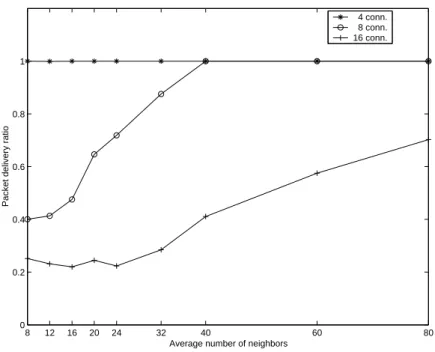
(8) of the work produced by the multihop network. • End-to-end delay: the total delay experienced by a packet that successfully reached the destination node. The end-to-end delay can be further broken down into – MAC delay: the delay due to the 802.11 Medium Access Control procedure. – Routing delay: the delay due to the DSR routing protocol, including the initial route discovery time. – Transmission delay: the time spent in radio transmission.. IV. Performance Evaluations In this section, we evaluate the impact of the number of neighbors on the performance of the wireless multihop ad hoc networks. Since we keep the area and the number of nodes fixed, as the number of neighbors increases, the network becomes less of a multihop network and more of a single-hop network.. Packet delivery ratio and hop-put 4 conn. 8 conn. 16 conn. 1. 0.8 Packet delivery ratio. A.. 0.6. 0.4. 0.2. 0. 8. 12. 16. 20. 24. 32. 40 Average number of neighbors. 60. 80. Figure 1: Packet delivery ratio vs. average number of neighbors. 8.

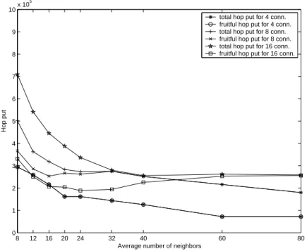
(9) Fig. 1 shows the packet delivery ratio versus the average number of neighbors when there are 4, 8, and 16 CBR connections. The number of neighbors is varied by changing the transmission range. From Fig. 1, we see that the packet delivery ratio is 1 when the traffic load is light (4 CBR connections). As the traffic load is moderate to high (8 to 16 CBR connections), the packet delivery ratio becomes lower when the transmission range is decreased. In the case that the packet delivery ratio is lower than 1, some packets are queued or discarded somewhere in the network. We further looked into the detailed operations and found that packets are lost at the intermediate (or relay) nodes but not at the sources. Since the number of hops that a packet needs to travel is larger when the transmission range becomes smaller, we suspect that the throughput degradation at small transmission range is due to increased radio transmissions. Higher loading at the radio/MAC layer increases the probability of frame collision and decreases the network performance. 5. 10. x 10. total hop put for 4 conn. fruitful hop put for 4 conn. total hop put for 8 conn. fruitful hop put for 8 conn. total hop put for 16 conn. fruitful hop put for 16 conn.. 9. 8. 7. Hop put. 6. 5. 4. 3. 2. 1. 0. 8. 12. 16. 20. 24. 32. 40 Average number of neighbors. 60. 80. Figure 2: Total hop-put and fruitful hop-put vs. average number of neighbors for 4, 8, 16 connections. In Fig. 2, we plot hop-puts (number of radio transmissions) vs. average number of. 9.

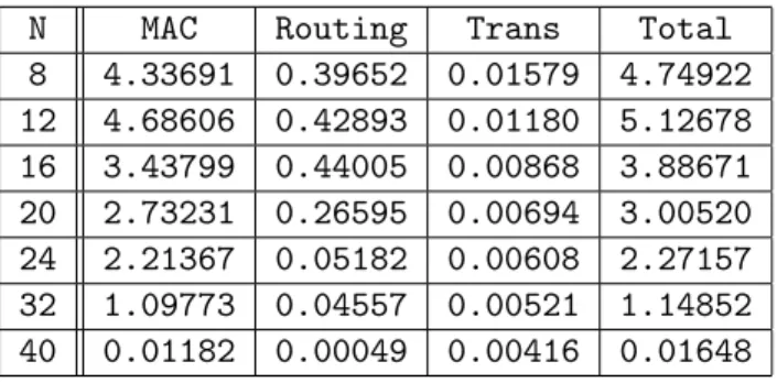
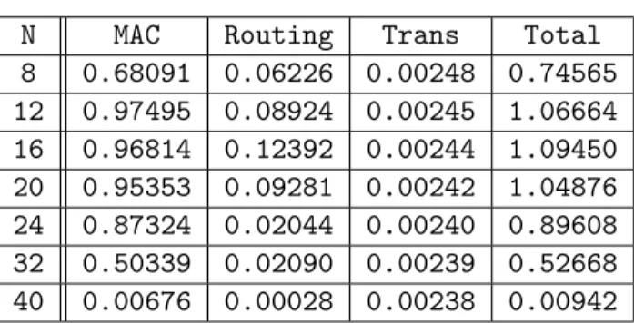
(10) neighbors. Both the fruitful hop-put and the total hop-put are shown. The number of neighbors is increased by increasing the transmission range. We can see that at a smaller transmission range, there is a bigger difference in the fruitful hop-put and the total hopput. In other words, more successful radio transmissions are spent on packets that do not reach their final destinations. The reason that some packets cannot reach their destination is due to the increased traffic loading at the MAC layer when the hop distance between the source and the destination becomes larger (due to shorter transmission range) and also due to the creation of more congested nodes. When the transmission range is high enough (near a single-hop network), a successful radio transmission is a successful CBR packet delivery. The network does not waste the network resource and this will improve the network performance. This shows that a larger transmission range achieves better network performance. When all nodes are in transmission range of each other, the best network performance can be achieved. This result is in agreement with that in [9]. Table 1: Breakdown of end-to-end packet delay N 8 12 16 20 24 32 40. MAC 4.33691 4.68606 3.43799 2.73231 2.21367 1.09773 0.01182. Routing 0.39652 0.42893 0.44005 0.26595 0.05182 0.04557 0.00049. Trans 0.01579 0.01180 0.00868 0.00694 0.00608 0.00521 0.00416. Total 4.74922 5.12678 3.88671 3.00520 2.27157 1.14852 0.01648. Table 1 shows the end-to-end packet delivery delay and its breakdown into MAC delay, routing delay, and transmission delay, at various values of the average number of neighbors. There are 8 CBR connections. Table 2 shows the per-hop packet delivery delay and its breakdown into MAC delay, routing delay, and transmission delay, at various values of the average number of neighbors.. 10.

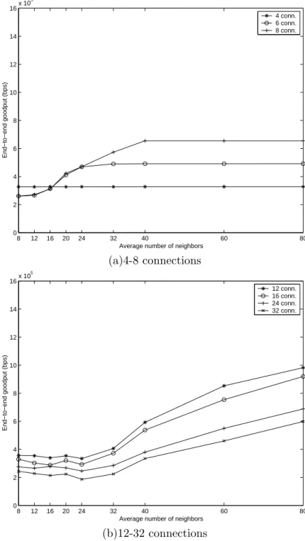
(11) Table 2: Breakdown of per-hop packet delay N 8 12 16 20 24 32 40. MAC 0.68091 0.97495 0.96814 0.95353 0.87324 0.50339 0.00676. Routing 0.06226 0.08924 0.12392 0.09281 0.02044 0.02090 0.00028. Trans 0.00248 0.00245 0.00244 0.00242 0.00240 0.00239 0.00238. Total 0.74565 1.06664 1.09450 1.04876 0.89608 0.52668 0.00942. From Tables 1 and 2, we know that the physical transmission delay and routing delay are small and total packet delivery delay is dominated by the MAC delay. The MAC delay decreases when the traffic load is low. When the transmission range is large, the network approaches the one-hop environment, and the total packet delivery delay will be small because the MAC layer traffic loading is relatively low.. B.. End-to-end goodput. In Fig. 1, we note that at 4 CBR connections, the packet delivery ratio remains at one independent of the transmission range or the number of neighbors. This is because 4 CBR connections offer light load to the network and the network has enough capacity to handle them. However, the packet delivery ratio does not tell us the maximum data rate that the network can deliver. Instead, the goodput is the appropriate metric for the carried data rate. Fig. 3 shows the end-to-end goodput versus the average number of neighbors. We display the results in two parts. • case (a): The offered load is light (4, 6, 8 CBR connections). The end-to-end goodput reaches the highest possible value (the offered load) when the number of neighbors is large. As the number of neighbors decreases, the end-to-end goodput decreases (except for the lightly loading case of 4 CBR connections). Again, the decrease in goodput is due to the increase in MAC loading at a multihop environment. Note that the goodput stays constant when the number of neighbors is 11.

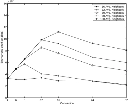
(12) large. This indicates that the network capacity if larger than the traffic load. • case (b): The offered load is moderate to heavy (12, 16, 24, 32 CBR connections). In Fig. 3 (b), as the number of CBR connections increases, the end-to-end goodput decreases. When the average number of neighbors is large, the end-to-end goodput suffers from the traffic increase due to the increased connections. When the average number of neighbors is small, the end-to-end goodput suffers from additional traffic increase due to the multihop transmissions. Note that in this case the goodput could be even lower than when the traffic load is light. Nonetheless, given a particular CBR connection number, the goodput is still higher when the network is closer to a single-hop network. We investigated the effect of routing on the above results by checking the following. In our simulation when the transmission range is 122m, the average number of neighbors is 8, and there is no route broken problem. We also investigated the impact of AODV and DSR routing protocols on the end-to-end goodput. We found that there is little difference in using either DSR or AODV. We redraw Fig. 3 into Fig. 4 to show how the end-to-end goodput changes as the offered load increases. The curve at the top of the figure corresponds to a single-hop network (100 average neighbors). As the number of connections increases from 4 to 12, the goodput increases proportionally to the connection number. The maximum goodput (approximately 1.12 Mbps) is achieved at around 16 connections, then it starts to decay. When the number of neighbors increases (i.e., moving towards a multihop network), the goodput starts to decay at points where the connection numbers are smaller. It clearly indicates that IEEE 802.11 multihop networks deliver lower goodput than single-hop networks. In Fig. 5, we plot the total hop-put vs. the connection number. It can be seen that the total hop-put is increased when the transmission range is decreased. In Table 3, we show, at 8 CBR connections, the spatial reuse factor (defined as the hop-put of a 12.

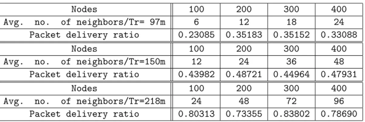
(13) multihop network divided by the hop-put of a single-hop network) and the hop increase factor (the number of hops a received packet has travelled) at different average number of neighbors (N ). It is clear that there does exist a spatial reuse of radio channels in a multihop network. However, this increase in spatial reuse is not high enough to match the increase in MAC layer traffic due to the hop count increase. This explains the goodput degradation as shown in Fig. 3. Table 3: Spatial reuse factor vs. Hop increase factor (8 CBR connections).. Spatial reuse factor Hop increase factor. C.. N=8 3.48 6.36. N=16 2.21 3.56. N=32 1.91 2.18. Effect of node density. We next investigate the effect of the node density. The node density is adjusted by fixing the area and varying the number of nodes. Note that the average number of neighbors is also changed in this way. Table 4 shows the packet delivery ratio versus the number of nodes for 16 CBR connections. Since there are fixed numbers of connections, most nodes function as relay nodes. In other words, as the number of nodes increases, the offered traffic remains the same. Table 4: Packet delivery ratio at different numbers of relay nodes Nodes Avg. no. of neighbors/Tr= 97m Packet delivery ratio Nodes Avg. no. of neighbors/Tr=150m Packet delivery ratio Nodes Avg. no. of neighbors/Tr=218m Packet delivery ratio. 100 6 0.23085 100 12 0.43982 100 24 0.80313. 200 12 0.35183 200 24 0.48721 200 48 0.73355. 300 18 0.35152 300 36 0.44964 300 72 0.83802. 400 24 0.33088 400 48 0.47931 400 96 0.78690. From the results in Table 4 we know that the packet delivery ratio has no significant 13.

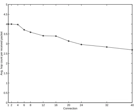
(14) variation when the number of nodes is increased. Therefore we can say that the packet delivery ratio is mainly influenced by the transmission range and the network load and not by the number of neighbors. In other words, it is misleading to say that the network performance depends on the number of neighbors if the variation of the number of neighbors does not reflect the change in the transmission range or the loading.. D.. Network capacity versus loading. Fig. 6 shows the hop-put versus the number of offered connections when the average number of neighbors is 16. When the number of connections is small, the network can carry all offered traffic. When the number of connections exceeds a certain value (say, six in the Fig. 6), the fruitful hop-put starts to decrease and the wasted hop-put is increased, while the total hop-put is increased slowly. We see that the total hop-put has a upper limit, which represents the MAC frame delivery capacity of the network. When the loading is heavy, the network capacity is spent more on carrying packets that fail to reach their destinations. This phenomenon has something to do with the routing mechanism. In DSR, if a packet fails several times in attempting to accessing the medium, it would claim the route broken and report a route error to the source node. The source node would then try another route which is more likely to be a longer route. As the traffic load is heavy, more routes are claimed broken and retried. More routes will be longer than before. All these effects increase the wasted hop-put. Fig. 7 plots the average number of radio transmissions (hop-count) for a successfully received packet versus the number of connections. This hop-count indicates the hop distance that a successfully received packet has travelled. We find that the average hop count decreases as the number of connections increases. Since the average distance between a source-destination node pair is kept constant at different connection numbers, this result indicates that successfully received packets are mainly from connections with shorter hop-counts. 14.

(15) V. Conclusions We have studied the performance of a wireless multihop ad hoc networks which uses the IEEE 802.11 DCF as its MAC mechanism. We found that the end-to-end goodput of the multihop network is in general lower than that of a single-hop network. The main reason is that the channel spatial reuse factor gained from the multihop network does not match the increase in additional transmission hops that a packet needs to travel in a multihop network. We also found that the dominating packet delivery delay is the MAC delay. For a multihop network, its MAC frame delivery capacity is fixed and dependent on its spatial reuse factor. If the offered load increases, less capacity will be spent on delivering packets that eventually reach their destinations and hence resulting in lower ene-to-end goodput. We also show that it is sometimes misleading to characterize the wireless network performance by the average number of neighbors since different numbers of neighbors do not necessarily mean different level of interfering traffic or different source-destination hop counts. There are many other factors (e.g., routing, mobility) that affect the performance of a multihop ad hoc network and they are topics for future research.. 15.

(16) 5. 16. x 10. 4 conn. 6 conn. 8 conn. 14. End−to−end goodput (bps). 12. 10. 8. 6. 4. 2. 0. 8. 12. 16. 20. 24. 32. 40 Average number of neighbors. 60. 80. (a)4-8 connections 5. 16. x 10. 12 conn. 16 conn. 24 conn. 32 conn.. 14. End−to−end goodput (bps). 12. 10. 8. 6. 4. 2. 0. 8. 12. 16. 20. 24. 32. 40 Average number of neighbors. 60. 80. (b)12-32 connections Figure 3: The end-to-end goodput versus different number of neighbors.. 16.

(17) 5. 16. x 10. 16 Avg. Neighbors 32 Avg. Neighbors 60 Avg. Neighbors 80 Avg. Neighbors 100 Avg. Neighbors. 14. End−to−end good put (bps). 12. 10. 8. 6. 4. 2. 0. 4. 6. 8. 12. 16. 24. 32. Connection. Figure 4: The end-to-end goodput versus different loads.. 5. 10. x 10. 16 Avg. Neighbors 32 Avg. Neighbors 60 Avg. Neighbors 80 Avg. Neighbors 100 Avg. Neighbors. 9. 8. 7. Hop put. 6. 5. 4. 3. 2. 1. 0. 4. 6. 8. 12. 16. 24 Connection. Figure 5: The total hop- put versus different loads.. 17. 32.

(18) 5. x 10. 10. total hop put wasted hop put fruitful hop put. 9. 8. 7. Hop put. 6. 5. 4. 3. 2. 1. 0. 1 2. 4. 6. 8. 12. 16. 20 24 Connection. 32. 40. Figure 6: The hop-puts versus different loads.. 5. 4.5. Avg. hop count per received packet. 4. 3.5. 3. 2.5. 2. 1.5. 1. 0.5. 0. 1 2. 4. 6. 8. 12. 16. 20 24 Connection. 32. 40. Figure 7: The average hop count per received packet versus different loads.. 18.

(19) References [1] T-C. Hou and T.J. Tsai, ”An Access-Based Clustering Protocol for Multihop Wireless Ad Hoc Networks,” IEEE Journal on Selected Areas in Communication, Vol. 19, No. 7, pp. 1201-1210, July, 2001. [2] L. Kleinrock and J. Silvester, ”Optimal Transmission Radii for Packet Radio Networks or Why Six is a Magic Number,” Proceedings of the IEEE National Telecommunications Conference, December 1978, pp. 4.3.1-4.3.5. [3] T-C. Hou and V.O.K. Li, ”Transmission Range Control in Multihop Packet Radio Network,” IEEE Transactions on Communication, Vol. Com-34, No. 1, January 1986, pp. 38-44. [4] H. Takagi and L. Kleinrock, ”Optimal Transmission Ranges for Randomly Distributed Distributed Packet Radio Terminals,” IEEE Transactions on Communications, Vol. Com-32, No. 3, March 1984. [5] S. Xu and T. Saadawi, ”Does the IEEE 802.11 MAC Protocol Work Well in Multihop Wireless Ad Hoc Netwoks ?,” IEEE Communication Magazine, June 2001, pp. 130137. [6] M. Natkaniec and A.R. Pach, ”An Analysis of the Backoff Mechanism used in IEEE 802.11 Networks,” Proc. Fifth IEEE Symposium on Computers and Communications, 2000, pp. 444-449. [7] M. Natkaniec and A. R. Pach, ”An Analysis of the Influence of the Threshold Parameter on IEEE 802.11 Network Performance,” Wireless Communications and Networking Conference, WCNC, 2000 IEE, Vol. 2, pp. 819-823. [8] S. Sharma, K. Gopalan and N. Zhu, ”Quality of Service Guarantee on 802.11 Networks,” Hot Interconnects 9, 2001. pp. 99-103. 19.

(20) [9] E. Dutkiewicz, ”Impact of Transmission Range on Throughput Performance in Mobile Ad Hoc Networks,” IEEE International Conference on Communications, Vol. 9, 2001, pp. 2933-2937. [10] E.M. Royer, P.M. Melliar-Smith and L.E. Moser, ”An Analysis of the Optimum Node Density for Ad Hoc Mobile Networks,” Proc. IEEE ICC 2001, Vol. 3, pp. 857-861. [11] L. Bajaj, M. Takai, R. Ahuja, K. Tang, R. Bagrodia and M. Gerla, Glomosim: A Scalable Network Simulation Environment. CSD Technical Report, UCLA, 1997. [12] IEEE Std. 802.11, ”Wireless LAN Media Access Control(MAC) and Physical Layer(PHY) Specifications,” 1999. [13] L. Munoz, M. Garcia, J. Choque, R. Aquero, ”Optimizing Internet Flows over IEEE 802.11b Wireless Local Area Networks: A Performance-Enhancing Proxy Based on Forward Error Correction,” IEEE Communications Magazine, December 2001, pp. 60-67. [14] G. Bianchi, ”Performance Analysis of the IEEE 802.11 Distributed Coordination Function,” IEEE Journal on Selected Areas in Communications, Vol. 18, NO. 3, March 2000, pp. 535-547. [15] K. Fall and K. Varadhan, Eds., ”ns notes and documentation.,” (1998) VINT Project, University California, Berkely, CA, LBL, USC/ISI, and Xerox PARC. [Online]. Available WWW: http://www-mash.cs.berkeley.edu/ns/. [16] B. Tuch, Development of WaveLAN, an ISM band wireless LAN, ATT Technical Journal, 72(4):27-33, July/August 1993. [17] D.B. Johnson and D. Maltz, ”Dynamic Source Routing in Ad Hoc Wireless Networks,” in Mobile Computing, Kluwer Academic Publ. 1996. 20.

(21) [18] D. A Maltz, J. Broch, J. Jetoheva and D. B. Johnson, ”The Effect of On-Demand Behavior in Routing Protocols for Multihop Wireless Ad Hoc Networks,” IEEE Journal on Selected Areas in Communications, Vol. 17. No. 8, August 1999, pp. 1439-1453.. 21.

(22)