郵票問題的研究

全文

(1)國立交通大學應用數學系碩士論文. 郵票問題的研究 A Study of Stamp Problem. 研究生：周俊全指導老師：傅恆霖. 教授. 中華民國九十六年六月.

(2) 郵票問題的研究 A Study of Stamp Problem 研究生：周俊全指導教授：傅恆霖. Student：Chun-Chuan Chou 教授. Advisor：Dr. Hung-Lin Fu. 國立交通大學應用數學系碩士論文. A Thesis Submitted to Department of Applied Mathematics College of Science National Chiao Tung University in Partial Fulfillment of the Requirements for the Degree of Master in Applied Mathematics June 2007 Hsinchu, Taiwan, Republic of China. 中華民國九十六年六月.

(3) 郵票問題的研究研究生：周俊全. 指導教授：傅恆霖教授. 國立交通大學應用數學系. 摘要所謂的郵票問題是出版一套每一張面額皆不同的郵票，使得面額總和以內的每一個數都可以用彼此相連不分散的郵票湊出來。舉例來說，假如我們要發行一套最多三張郵票，面額分別是一元、二元和四元，則我們可以湊出一到七元的郵票，而且每一種組合的郵票彼此都是相連不分散的。由上述的概念，我們可以把郵票問題的想法延伸到 graph labeling 上，用以下的方式：找一個圖 G 的 labeling 函數 ϕ : V (G ) → Ν 使得對於 1 到值和內的每一個值 k，必定存在一個值和為 k 的連通子圖 H。這樣的 labeling 方式就稱為圖 G 的 IC-著色，圖 G 的所有 IC-著色中最大的值和就是圖 G 的 IC-指標。在此篇論文當中，我們主要研究某些圖的 IC-著色和改善圖的指標的上界和下界。還有，我們也考慮當 ϕ [V (G ) ] = ⎡⎣1, V (G ) ⎤⎦ 的情形，並研究是否圖 G 具有 IC-著色；如果有的話，圖 G 就稱為可和飽和的。. i.

(4) A Study of Stamp Problem Student: Chun-Chuan Chou. Advisor: Hung-Lin Fu. Department of Applied Mathematics. Department of Applied Mathematics. National Chiao Tung University. National Chiao Tung University. Hsinchu, Taiwan 30050. Hsinchu, Taiwan 30050. Abstract The so-called stamp problem is to produce a set of stamps with distinct values such that we can obtain consecutive values by using distinct combinations of stamps from the given set. For example, if we are allowed to use at most three stamps from a set of stamps with value set {1, 2, 4}, then we have consecutive values 1, 2, · · · , 7. By way of the notion mentioned above, we can extend the idea of stamp problem to graph labeling in the following way : find a labeling of G, ϕ : V (G) → N , such P that for each valuePk ∈ [1, v∈V (G) ϕ(v)], there exists a connected subgraph H whose total value u∈H(G) ϕ(u) = k. The labeling obtained above is called an IC-coloring of G and the maximum value of an IC-coloring of G is the IC-index of G. In this thesis, we mainly study the IC-coloring of certain graphs and improve their known upper bounds and/or lower bounds, respectively. Moreover, we also consider the case when ϕ[V (G)] = [1, | V (G) |] and study whether the graph G has an IC-coloring, if so, G is said to be sum-saturable.. ii.

(5) Acknowledgement 此篇論文的完成，首先感謝我的指導教授傅恆霖老師，在我撰寫論文這段時間的細心指導與諄諄教誨。因為我ㄧ方面要教書，另一方面又要寫論文，一天二十四小時真的是不夠用，所幸老師的通融，在百忙之中另外安排時間研討我的論文，也協助我解決一些問題，讓我在學習研究的過程中受益良多，在此我由衷地感謝老師。其次我要感謝黃大原老師、陳秋媛老師以及翁志文老師，在我修課期間耐心指導與關心，最要感謝的是黃明輝學長與郭志銘學長在我寫論文時提供諮詢與建議，也要感謝陳宏賓學長、嚴志弘學長、張嘉芬學姊、詹棨丰學長等的幫助，使我在研究的過程中順利不少，以及宗翰、元勳、秋美、景堯、怡菁、書于、冠成這些同學，和他們一同研究課業、一起聚餐和遊玩，情感如同兄弟姐妹般，讓我留下許多美好的回憶。最後要感謝是我的家人，在我讀書的這段時間，老婆身兼嚴父慈母的角色，照顧兩個兒子無微不至，還有我的母親也時時鼓勵我要不斷精進，感謝他們背後的支持，讓我無後顧之憂地朝著求學目標前進，謝謝我摯愛的家人。. iii.

(6) Contents Abstract (in Chinese). i. Abstract (in English). ii. Acknowledgement. iii. Contents. iv. List of Figures. v. 1 Introduction. 1. 1.1. Preliminaries . . . . . . . . . . . . . . . . . . . . . . . . . . . . . . . . . .. 3. 1.2. Known Results . . . . . . . . . . . . . . . . . . . . . . . . . . . . . . . . .. 4. 1.2.1. Saturating labeling . . . . . . . . . . . . . . . . . . . . . . . . .. 4. 1.2.2. IC-coloring. 5. . . . . . . . . . . . . . . . . . . . . . . . . . . . . . .. 2 Saturating labelings of certain graphs. 7. 2.1. Constructive proofs of some graphs . . . . . . . . . . . . . . . . . . . . . .. 2.2. Palmerworm P W (n) . . . . . . . . . . . . . . . . . . . . . . . . . . . . . . 12. 3 Improved bounds of IC-index of some graphs. 7. 15. 3.1. Path Pn . . . . . . . . . . . . . . . . . . . . . . . . . . . . . . . . . . . . . 15. 3.2. Cycle Cn . . . . . . . . . . . . . . . . . . . . . . . . . . . . . . . . . . . . . 18. 3.3. Double-stars DS(m, n) . . . . . . . . . . . . . . . . . . . . . . . . . . . . . 21. 3.4. Corollaries of known results . . . . . . . . . . . . . . . . . . . . . . . . . . 23. 3.5. Improved lower bounds of some Graphs . . . . . . . . . . . . . . . . . . . . 24. 4 Conclusion. 27. iv.

(7) List of Figures 1. Stamp problem. . . . . . . . . . . . . . . . . . . . . . . . . . . . . . . . . .. 1. 2. Two distinct maximum IC-colorings of C4 . . . . . . . . . . . . . . . . . . .. 2. 3. An example of G and G + v with M (G + v) 6= 2M (G) + 1 . . . . . . . . . .. 6. 4. λ-label of vertices of Petersen graph. . . . . . . . . . . . . . . . . . . . . . 10. 5. λ-labelings of DS(2, 3), and DS(3, 3). . . . . . . . . . . . . . . . . . . . . . 12. 6. Palmerworm P W (8) containing a path P8 . . . . . . . . . . . . . . . . . . . 12. 7. Labeling of Palmerworm P W (n). . . . . . . . . . . . . . . . . . . . . . . . 13. 8. Labeling of Palmerworm P W (9). . . . . . . . . . . . . . . . . . . . . . . . 14. 9. Label 1 and 2 assigned to the end-vertices of Pn . . . . . . . . . . . . . . . 15. 10. The IC-coloring of the path Pn. 11. The improved lower bound of path P9 . . . . . . . . . . . . . . . . . . . . . 17. 12. Maximal IC-colorings of C3 , C4 , C5 and C6 . . . . . . . . . . . . . . . . . . . 18. 13. The IC-colorings of the cycle Cn . . . . . . . . . . . . . . . . . . . . . . . . 19. 14. Double-star DS(2, n) . . . . . . . . . . . . . . . . . . . . . . . . . . . . . . 21. 15. Lower bound of double-star DS(m, n) . . . . . . . . . . . . . . . . . . . . . 21. 16. IC-coloring of K(m, n) . . . . . . . . . . . . . . . . . . . . . . . . . . . . . 24. 17. IC-coloring of the complete tripartite K(a, b, c) . . . . . . . . . . . . . . . . 25. 18. The central labels are 1 when n ≤ 6 and 6 when n ≥ 7. . . . . . . . . . . . 26. . . . . . . . . . . . . . . . . . . . . . . . . 17. v.

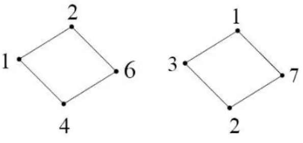
(8) 1. Introduction. Consider the following simple mathematical puzzle from Bolt’s book [2] : A country wishes to issue a block of four stamps, each with the shape of an equilateral triangle of unit side length. (illustrated in Figure 1) How should the values a, b, c and d be assigned so that one could get a connected group of stamps of total value k for each k = 1, 2, · · · , 10 ? This is the well-known Stamp Problem.. Figure 1: Stamp problem. It is easily verified that the set {a, b, c, d} must equal {1, 2, 3, 4}. And, it is equivalent to the problem of assigning positive integer labels to the vertices of K(1, 3) in such a way that for each integer k = 1, 2, · · · , 10, there is a connected subgraph whose labels sum to k. Moreover, we can think about this question for various classes of graphs in such a way to assign integer labels to the vertices. For example, the complete graph Kn , the cycle Cn , the path Pn , · · ·, and so on, and each leads to a graph labeling problem of the following type (Fink [3]).. Given a connected graph G having p vertices, is it possible to assign labels 1, 2, · · · , p to the vertices in such a way that for each k = 1, 2, · · · , p(p + 1)/2, G contains a connected subgraph whose labels sum to k ?. We find out that not every graph could label vertices in such a way. A labeling of a graph G of order p is a bijection λ : V (G) → [1, p], the integer λ(v) is called the λ-label P of v, and for each subgraph H of G, the sum v∈V (H) λ(v) will be denoted by λ(H) and P called the λ-value of H. We will use the notation ∆p to represent pj=1 j. If λ is a labeling 1.

(9) of a connected graph G of order p, and if, for each k ∈ [1, ∆p ], G has a connected subgraph H of λ-value k, then we say λ is a saturating labeling of G, or G has a λ − labeling. Any graph for which a saturating labeling exists will be called a sum-saturable graph. However, let’s consider another coloring type to the vertices of a graph G. Given a function f : V (G) → N is called a coloring of G. Let H be a subgraph of G. We define P fs (H) = v∈V (H) f (v). In particular, we denote fs (G) by S(f ) if H = G. A function f : V (G) → N is called an IC-coloring of G if for any integer k ∈ [1, S(f )], there is a connected subgraph H of G such that fs (H) = k. Note that any connected graph admits IC-coloring. For example, the function f : V (G) → N defined by f (v) = 1 for all v ∈ V (G) is an IC-coloring with the sum S(f ) = n. Here, for any integer k ∈ [1, n], a connected subgraph H of G with exactly k vertices will satisfy the condition fs (H) = k. The IC-index of a graph G, denoted by M (G), is defined to be M (G) = max{S(f ) | f is an IC-coloring of G}. Any IC-coloring f : V (G) → N for which S(f ) = M (G) will be called a maximum ICcoloring of G. A maximum IC-coloring of a graph is not necessarily unique, as illustrated in Figure 2.. Figure 2: Two distinct maximum IC-colorings of C4 . However, in any IC-coloring of a graph G, one has to assign 1 to the vertices which is not cut-vertices; otherwise, the number S(f ) − 1 can not be obtained from any connected subgraph of G. The problem of finding IC-coloring of finite graphs is related to the postage stamp problem in the number theory, which has been extensively studied in the literature [1, 4, 5, 6, 7] 2.

(10) 1.1. Preliminaries. In this section, we first introduce the terminologies and definitions of graphs. For details, the readers may refer to the book “Introduction to Graph Theory” by D. B. West [10]. A graph G is a triple consisting of a vertex set V (G), an edge set E(G), and a relation that associates with each edge two vertices called its endpoints. A loop is an edge whose endpoints are equal. Multiedges are edges having the same pair of endpoints. A simple graph is a graph without loops or multiedges. In this thesis, all the graphs we consider are simple. The cardinality of the vertex set V (G), |V (G)|, is called the order of G, and the cardinality of the edge set E(G), |E(G)|, is called the size of G. If e = (u, v) (uv in short) is an edge of G, then e is said to be incident to u and v. We also say that u and v are adjacent to each other. For every v ∈ V (G), N (v) denotes the neighborhood of v, that is, all vertices of N (v) are adjacent to v. The degree of v, deg(v) = |N (v)|, is the number of neighbors of v. A cut-vertex of a graph G is a vertex whose deletion will disconnect G. An induced subgraph of a graph G is a subgraph obtained by deleting a set of vertices. A spanning subgraph of G is a subgraph H with V (H) = V (G). A matching of size k in G is a subgraph of k pairwise vertex disjoint edges. If a matching covers all vertices of G, then it is a perfect matching. A factor of a graph G is a spanning subgraph of G. A k-factor is a spanning subgraph with each degree equal to k. Then a 1-factor and a perfect matching are almost the same thing. A path is a simple graph whose vertices can be ordered so that two vertices are adjacent if and only if they are consecutive in the list. And a path of order n is denoted by Pn . A cycle is a graph with an equal number of vertices and edges whose vertices can be placed around a circle so that two vertices are adjacent if and only if they appear consecutively along the circle. A cycle with n vertices is denoted by Cn . A Hamiltonian graph is a graph with a spanning cycle, also called a Hamiltonian cycle. A wheel with n spokes is obtained by the join operation Cn + K1 . It is denoted by Wn . If G has a u, v-path, then the distance from u to v, written by d(u, v), is the least 3.

(11) length of a u, v-path. The diameter of G is maxu,v∈V (G) d(u, v). A graph with no cycle is acyclic. A tree is a connected acyclic graph. A spanning tree is a spanning subgraph that is a tree. Trees of diameter three are called double-star. These graphs have two central vertices plus leaves. We will use DS(m, n) to denote the double-star whose two central vertices have degrees m and n, respectively. (defined by [9]) A complete graph is a simple graph whose vertices are pairwise adjacent; the complete graph with n vertices is denoted by Kn . A graph G is bipartite if V (G) is the union of two disjoint independent sets called partite sets of G. A graph G is m-partite if V (G) can be expressed as the union of m independent sets. A complete bipartite graph is a bipartite graph such that two vertices are adjacent if and only if they are in different partite sets. When the sets have the sizes m and n, the complete bipartite graph is denoted by K(m, n). Similarly, the complete n-partite graph is denoted by K(m1 , m2 , ..., mn ) when the n partite sets have the sizes m1 , m2 , · · · , mn . In particular, the complete bipartite graph K(1, n) is called star and is denoted by ST (n) for any n ≥ 1.. 1.2 1.2.1. Known Results Saturating labeling. Fink showed that for any n ≥ 4, the path Pn is not sum-saturable[3] . However, all cycles, Hamiltonian graphs, and complete bipartite graphs are sum-saturable according to the following two results (Fink [3]). Theorem 1.1. [3] If G is a 2-connected graph having either a 1-factor or a near-onefactor, then G is sum-saturable.. 4.

(12) Theorem 1.2. [3] A connected graph G of order p is sum-saturable if it has a vertex v for which (1) deg(v) ≥ 1 + dlog2 (p − 1)e, and (2) there is a (proper) subset S of N (v) such that |S| = dlog2 (p − 1)e and G − S is connected.. 1.2.2. IC-coloring. In 1995, Penrice [8] introduced the concept of stamp covering of G as follows : for an integer k > 0, a labeling f : V (G) → N is called a k-labeling if for any integer j, 1 ≤ j ≤ k, there exists a connected induced subgraph H of G with fs (H) = j. Then, M (G), the stamp covering number of G, is the largest k ∈ N such that G has a k-labeling. He also showed that (1) M (Kn ) = 2n − 1. (2) M (K(1, n)) = M (ST (n)) = 2n + 2, for all n ≥ 2. (3) For positive integer n ≥ 4, (n2 + 6n − 4)/4 ≤ M (Pn ) ≤ n(n + 1)/2 − 1. Around 10 years later, this notion was rediscovered by Salehi et al. [9] and the names IC-coloring and IC-index take place of stamp covering and stamp covering number, respectively. We list some of the results obtained so far. Theorem 1.3. [9] For any integer n ≥ 2, the IC-index of the complete bipartite graph K(2, n) is 3 · 2n + 1. Theorem 1.4. [9] For any integer n ≥ 3, the IC-index of the wheel Wn satisfies the following inequalities : 2n + 2 ≤ M (Wn ) ≤ 2n + n(n − 1) + 1 for n ≥ 3. Theorem 1.5. [3, 8, 9] For any n ≥ 3, n(n + 1)/2 ≤ M (Cn ) ≤ n(n − 1) + 1. And M (Cn ) = n(n − 1) + 1 when n = 3, 4, 5, 6, 8, 9. 5.

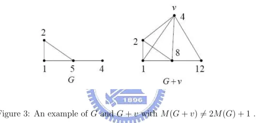
(13) Observation 1.6. [9] If H is a subgraph of G, then M (H) ≤ M (G). Observation 1.7. [9] If v(G) is the number of connected induced subgraphs of G, then M (G) ≤ v(G). Observation 1.8. [9] If M (G) = µ and v ∈ / V (G), then M (G + v) ≥ 2µ + 1. The inequality is sharp when G is the complete graph. That is, M (Kn+1 ) = 2M (Kn ) + 1. However, there are cases when equality does not hold. Consider the graph G in Figure 3. The graph has exactly 12 non-empty connected induced subgraphs with M (G) = 12. But, M (G + v) ≥ 27.. Figure 3: An example of G and G + v with M (G + v) 6= 2M (G) + 1 . In this thesis, we shall first study the saturating labelings in Chapter 2. Mainly, constructive labelings are given for those graphs which have good structures, for example, complete multipartite graphs. Then, in Chapter 3, focus our effort in improving the upper and/or lower bounds of the IC-index of some graphs obtained in an earlier paper by Salehi et al.[9]. 6.

(14) 2. Saturating labelings of certain graphs. Though the complete graphs Kn , the complete bipartite graphs K(m, n), the complete multipartite K(m1 , m2 , ...mn ) and Petersen graph satisfy with the conditions mentioned in Theorem 1.1 and Theorem 1.2, we provide constructive proofs.. 2.1. Constructive proofs of some graphs. Theorem 2.1. For any complete graph Kn , Kn is sum-saturable. Proof. Let V (Kn ) = {v1 , v2 , · · · , vn }, and define a labeling λ : V (Kn ) → N by λ(vi ) = i, P for each i ∈ [1, n]. Let k ∈ [1, ∆n ], where ∆n = ni=1 i = n(n+1) . It remains to show that 2 λ is a saturating labeling. (1) When 1 ≤ k ≤ n : The subgraph hλ−1 (k)i of Kn is a single vertex. (2) When k = n + i for 1 ≤ i ≤ n − 1 : The subgraph of Kn is consisted of two vertices, which are λ−1 (n), and λ−1 (i) such that the λ-value of the subgraph is k. (3) When k = n + (n − 1) + i for 1 ≤ i ≤ n − 2 : The subgraph of Kn is consisted of three vertices, which are λ−1 (n), λ−1 (n − 1), and λ−1 (i) such that the λ-value of the subgraph is k. We keep going on by this way: (n-1) When k = n + (n − 1) + (n − 2) + · · · + 3 + i for 1 ≤ i ≤ 2 : The subgraph of Kn is consisted of n − 1 vertices, which are λ−1 (n), λ−1 (n − 1), λ−1 (n − 2), · · · , λ−1 (3), and λ−1 (i) such that the λ-value of the subgraph is k. (n) When k = n + (n − 1) + (n − 2) + · · · + 3 + 2 + 1 : The subgraph of Kn is Kn itself. Since Kn is complete, any subgraph H induced by the vertices of Kn is also connected. Hence, Kn is sum-saturable.. 7.

(15) Theorem 2.2. For all positive integers m and n, the complete bipartite graph K(m, n) is sum-saturable. Proof. Assume that m ≥ n, and let Vm = {v1 , v2 , · · · , vm } and Vn = {vm+1 , vm+2 , · · · , vm+n } be the two partite sets of K(m, n), with |Vm | = m and |Vn | = n. Then we define a labeling P m+n λ : V (K(m, n)) → N by λ(vi ) = i, for each i ∈ [1, m + n]. Let ∆m+n = i=1 i = (m+n)(m+n+1) . 2. We proceed by induction on n. If |V1 | = 1, V1 = {vm+1 } and λ(vm+1 ) = m + 1, and P m+1 (m+1)(m+2) . We claim that K(m, 1) is sum-saturable. ∆m+1 = i=1 i = 2 (1) When k ∈ [1, m + 1] : The subgraph hλ−1 (k)i of K(m, 1) is a single vertex. (2) When k = (m + 1) + i, for 1 ≤ i ≤ m : The subgraph of K(m, 1) is consisted of two vertices, which are λ−1 (m + 1), and λ−1 (i) such that the λ-value of the subgraph is k. (3) When k = (m + 1) + m + i, for 1 ≤ i ≤ m − 1 : The subgraph of K(m, 1) is consisted of three vertices, which are λ−1 (m + 1), λ−1 (m), and λ−1 (i)} such that the λ-value of the subgraph is k. We keep going on by the same way: (m) When k = (m + 1) + m + (m − 1) + · · · + 3 + i for 1 ≤ i ≤ 2 : The subgraph of K( m, 1) is consisted of m vertices, which are λ−1 (m + 1), λ−1 (m), λ−1 (m − 1), · · · , λ−1 (3), and λ−1 (i) such that the λ-value of the subgraph is k. (m+1) When k = (m + 1) + m + · · · + 3 + 2 + 1 = ∆m+1 =. Pm+1 i=1. i=. (m+1)(m+2) 2. : The. subgraph is K(m, 1) itself. And we can easily check that any subgraph listed above is connected since every subgraph listed above has two partite sets except subgraphs with only one vertex. Hence, K(m, 1) is sum-saturable. Suppose K(m, k) is sum-saturable, then there exists a labeling λ of G such that λ(vi ) = i, for each i ∈ [1, m + k]. Suppose |Vm | = m and |Vn | = k, and we use ∆m+k to denote P m+k (m+k)(m+k+1) . i=1 i = 2 8.

(16) Consider the case when |Vn | = k + 1. We assign a label m + k + 1 to the vertex vm+k+1 . Since K(m, k) is sum-saturable, the subgraphs of K(m, k) with labels 1 to ∆m+k exist, and the subgraphs of K(m, k) are connected. When k = ∆m+k + i, for 1 ≤ i ≤ m + k, we can find the subgraph Hi of K(m, n) is consisted of a set of m + k vertices, which is {vm+k+1 , vm+k , vm+k−1 , · · · vm+1 , vm , vm−1 , · · ·, v2 , v1 } \ {v(m+k+1)−i } such that the λvalue of the subgraph is k. It is trivial that when k is equal to ∆m+k+1 , the subgraph is G itself. And we can easily check that the subgraphs mentioned above are connected since every subgraph Hi has also two partite sets . Thus, we know that the complete bipartite graph K(m, n) is sum-saturable. Corollary 2.3. For any n ≥ 2, the star ST (n) is sum-saturable. Proof. ST (n) is K(1, n). Corollary 2.4. For any n≥ 3, the wheel Wn is sum-saturable. Proof. Consider K(1, n) in Theorem 2.2. Theorem 2.5. For all positive integers m1 , m2 , · · · , mn , the complete multipartite graph K(m1 , m2 , · · · , mn ) is sum-saturable. Proof. Assume that m1 ≥ m2 ≥, · · ·, ≥ mn , and use Vm1 , V m2 , · · ·, Vmn to denote the partite sets of the complete multipartite graph G = K(m1 , m2 , · · · , mn ) with |Vm1 | = m1 , |Vm2 | = m2 , · · ·, |Vmn | = mn , and m1 + m2 + · · · + mn = p. Let λ be the labeling that assigns the labels 1, 2, · · ·, m1 to the vertices of Vm1 , and (m1 + 1), (m1 + 2), · · ·, (m1 + m2 ) to the vertices of Vm2 , and [(m1 + m2 ) + 1], [(m1 + m2 ) + 2], · · ·, [(m1 + m2 ) + m3 ] to the vertices of Vm3 , · · ·, and [(m1 + m2 + · · · + mn−1 ) + 1], [(m1 + m2 + · · · + mn−1 ) + 2], · · · [(m1 + m2 + · · · + mn−1 ) + mn ] to the vertices of Vmn . First, we only focus on the two partite sets Vm1 and Vm2 . Aided by the preceding proof of Theorem 2.2, we can easily check that G has a connected subgraph with λ-value S 1 +m2 +1) ]. Then, we regard Vm1 Vm2 as a new partite set U1 . Then, k ∈ [1, (m1 +m2 )(m 2 proceeding to do another two partite sets U1 and Vm3 , we can also check that G has a 1 +m2 +m3 +1) connected subgraph with λ-value k ∈ [1, (m1 +m2 +m3 )(m ]. 2. 9.

(17) Keeping going on by this technique mentioned above. Finally, we view the union of Vm1 , Vm2 , · · ·, Vmn−1 as a new partite set Umn −2 , and, consider the two partite sets Umn −2 and Vmn , we can still easily check that G has a connected subgraph of λ-value k ∈ [1, ∆p =. p(p+1) ]. 2. Hence, we conclude that the complete multipartite graph K(m1 , m2 , ...mn ) is sumsaturable. Proposition 2.6. The Petersen graph is sum-saturable.. Figure 4: λ-label of vertices of Petersen graph. Proof. Let V (G) = {v1 , v2 , · · · , v10 }. and F = {e1 , e2 , e3 , e4 , e5 }. Let λ be a labeling of G satisfying the condition that for each i ∈ [1, 5], one of the two vertices adjacent with the edge ei has label i and the other has 11 − i. Let k ∈ [1, ∆10 ], and let q and r be the nonnegative integers satisfying k = 11q + r, and 0 ≤ r ≤ 10. (1) If q = 0, there exists a single vertex vi such that λ(vi ) = i, for each i ∈ [1, 10]. (2) If q ≥ 1 and r ≥ 1, let λ(vj ) = r, we can find the subgraph H1 of G containing q edges {ej+1 , ej+2 , · · · , ej+q } of F plus vertex vj when 1 ≤ j ≤ 5, where j + q (mod 5). Also, when 6 ≤ j ≤ 10, we can find the subgraph H10 of G containing q edges {e11−j+2 , e11−j+4 , · · · , e11−j+2q } of F plus vertex vj , where 11 − j + 2q (mod 5) for q ∈ [1, 4]. One can check that H1 and H10 are both connected subgraphs of G.. 10.

(18) (3) If q ≥ 1 and r = 0, the subgraph H2 of G containing q edges {e1 , e2 , · · · , eq } of F such that λ(H2 ) = 11q. And we can easily check that H2 is a connected subgraph of G since G is 2-connected. Thus, the Petersen graph is sum-saturable. Fink [3] provided two sufficient conditions to check if a graph of order p is sumsaturable; such as the followings : (1) There exists v such that deg(v) ≥ 1 + dlog2 (p − 1)e, and (2) There is a (proper) subset S of N (v) such that |S| = dlog2 (p − 1)e and G − S is connected. In what follows, we shall check whether the double-star DS(m, n) is sum-saturable using the two conditions. Proposition 2.7. For 2 ≤ m ≤ n, the double-star DS(m, n) is sum-saturable except DS(2, 2), which is a path P4 . Proof. Let u and v be the central vertices of DS(m, n) with degree m and n, respectively. We first check the vertex v because it is the vertex with maximum degree in the double-star DS(m, n). For n ≥ m, we have 2n − 1 ≥ m + n − 1. One can check that 2n−1 ≥ 2n − 1 for n ≥ 4. Hence, we get the inequality : 2n−1 ≥ m+n−1. So, we have n−1 ≥ log2 (m+n−1). It is equivalent that n − 1 ≥ dlog2 (m + n − 1)e. Hence, the double-star DS(m, n) fits the condition (1). That is, n ≥ 1 + dlog2 (m + n − 1)e, when n ≥ 4. Now we check the condition (2). When we let S ⊆ N (v)\{u} with |S| = dlog2 (m + n − 1)e, DS(m, n) − S leads deg(v) to be at least 1. Hence, DS(m, n) − S is also connected. So, DS(m, n) is sum-saturable when n ≥ 4 and n ≥ m. Now, we check the double-star DS(2, 3) (see the left graph in Figure 5). It also satisfies the sufficient condition (1) when we check vertex v. Now, let S = {y | deg(y) = 1 for any. 11.

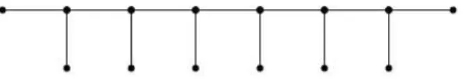
(19) vertex y ∈ N (v)}. Then, G − S is connected satisfying condition (2) because |S| = 2 and deg(v) = 3. For DS(3, 3), it follows by using the labelings in Figure 5.. Figure 5: λ-labelings of DS(2, 3), and DS(3, 3).. 2.2. Palmerworm P W (n). It is worth of noting that we can not use Fink’s conditions to show that DS(3, 3) is sum-saturable. Hence, it seems that there exists some sum-saturable graphs in which deg(v) ≤ dlog2 (|V (G)| − 1)e for any v ∈ V (G). Fortunately, we find a graph called palmerworm is sum-saturable, which is illustrated in Figure 6 . It is consisted with a path Pn and n − 2 vertices which are adjacent with the cut-vertices of Pn . We can check that deg(v) ≤ dlog2 (|V (G)| − 1)e for any v. Here, we denote the palmerworm by P W (n).. Figure 6: Palmerworm P W (8) containing a path P8 .. 12.

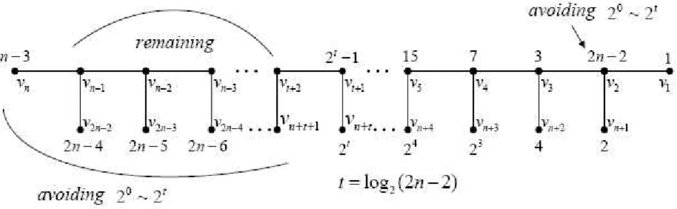
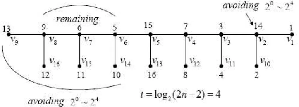
(20) Figure 7: Labeling of Palmerworm P W (n).. Theorem 2.8. A graph G = P W (n) is sum-saturable. Proof. Let V (G) = {v1 , v2 , v3 , · · · , v2n−2 } be the vertices of P W (n), and t = blog2 (2n − 2)c. Then there exists a λ labeling of P W (n) such as Figure 7. First, we label 1, 2, 4, · · · , 2t to the vertices v1 , vn+1 , vn+2 , · · · , vn+t , and λ(v3 ) = 1 + 2 = 3, λ(v4 ) = 1 + 2 + 4 = 7, · · ·, λ(vt+1 ) = 1 + 2 + · · · + 2t−1 = 2t − 1, respectively.. Secondly, the vertices. v2 , vn , v2n−2 , v2n−3 , · · · , vn+t+1 are respectively labeled with 2n − 2, 2n − 3, 2n − 4, 2n − 5, · · ·, until vertex vn+t+1 has been labeled; but avoiding 20 , 21 , · · · , 2t and the values given previously, i.e. if the same label of some vertex is w, then we give w − 1 to it and then going on. At last, the others are labeled with the remaining values randomly. Then we can easily check that P W (n) is sum-saturable.. 13.

(21) Figure 8: Labeling of Palmerworm P W (9).. Example 2.9. A graph G = P W (9) is sum-saturable, in which deg(v) ≤ dlog2 16e = 4 for any v ∈ G. Let V (P W (9)) = {v1 , v2 , · · · , v16 }. There exists a λ labeling as illustrated in Figure 8. It is necessary to check for any k ∈ [1, ∆9 = 136], there exists a connected subgraph H such that λ(H) = k. When k ∈ [1, 16], the subgraph is a single vertex. Next, when k ∈ [14, 17], [17, 24], [24, 39], [39, 70], [44, 85], [50, 102]and[59, 136], there still exists a connected subgraph H such that λ(H) = k. Hence, P W (9) is sum-saturable. Therefore, to find a necessary and sufficient condition for a graph to be sum-saturable is an interesting open problem.. 14.

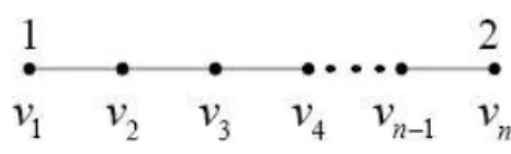
(22) 3. Improved bounds of IC-index of some graphs. First, we consider the IC-index of the path Pn . Since v(Pn ) = n(n + 1)/2 , the IC-index of Pn is less or equal to n(n + 1)/2. And M (Pn ) has a lower bound (2 + bn/2c)(n − bn/2c) + bn/2c − 1 [9]. The more n becomes, the more difficult it is to find out the bounds of IC-index of path Pn . Hence, we will search for the labels of vertices by using computer. Finally, we have a formulated type of the IC-coloring of path Pn .. 3.1. Path Pn. Lemma 3.1. For any n ∈ N, M (Pn ) ≤ n(n + 1)/2 − 1. Proof. Since Pn is a path of order n, let V (Pn ) = {v1 , v2 , · · · , vn }, where the vertices v1 , v2 , · · · , vn are sorted in order. Observe that v1 and vn are the only two end-vertices of Pn , and every vertex other than v1 , vn is a cut-vertex. Suppose f is a maximum ICcoloring of Pn such that M (Pn ) = µ. In order to produce µ − 1, we have to let f (v1 ) = 1 or f (vn ) = 1. Without loss of generality, we let f (v1 ) = 1. And to produced µ − 2, we have three cases : f (v2 ) = 1, f (vn ) = 1 or f (vn ) = 2. If f (v2 ) = 1 or f (vn ) = 1, 1 is repeated, and hence M (Pn ) ≤ n(n + 1)/2 − 1. If f (vn ) = 2, we can also produce µ − 3. To cover 3, 4, 5 and µ − 4, µ − 5, we consider the following cases :. Figure 9: Label 1 and 2 assigned to the end-vertices of Pn Case 1. f (v2 ) = 3 : We can produce 3, 4, and µ − 4. In order to produce µ − 5, we have to let f (vn−1 ) = 3 or f (v3 ) = 1. Since either 3 or 1 is repeated, we have the upper bound n(n + 1)/2 − 1. Case 2. f (vn−1 ) = 3 : 15.

(23) We can produce 3, 5 and µ − 5. To cover 4 and µ − 4, we will have f (v2 ) = 3, which is again repeated. Hence, M (Pn ) ≤ n(n + 1)/2 − 1. Case 3. f (vj ) = 3 for j 6= 1 and n : We can only produce the value 3. To cover 4, µ − 4 and µ − 5, we will have three choices for the pair v2 and vn−1 , which are (3, 3), (2, 2), (4, 2). Thus, number 1, 2, or 3 will be repeated in the three choices. Hence, we have improved the upper bound of M (Pn ). Aided by using computer, we have the following results. Without loss of generality, let V (Pn ) = {v1 , v2 , · · · , vn } and let the vertices are sorted from the left to the right. And the IC-indices of Pn are at least the sum of the vertices of Pn . (1) n = 3 : M (P3 ) = 1 + 3 + 2 = 6 (2) n = 4 : M (P4 ) ≥ 9 = 1 + 1 + 4 + 3 = 1 + 3 + 3 + 2 (3) n = 5 : M (P5 ) ≥ 13 = 1 + 1 + 4 + 4 + 3 = 1 + 3 + 1 + 6 + 2 = 1 + 5 + 3 + 2 + 2 (4) n = 6 : M (P6 ) ≥ 17 = 1 + 1 + 1 + 5 + 5 + 4 = 1 + 1 + 4 + 4 + 4 + 3 = 1 + 1 + 6+4+3+2 (5) n = 7 : M (P7 ) ≥ 23 = 1 + 1 + 9 + 4 + 3 + 3 + 2 = 1 + 3 + 6 + 6 + 2 + 3 + 2 (6) n = 8 : M (P8 ) ≥ 29 = 1 + 4 + 4 + 7 + 7 + 3 + 2 + 1 (7) n = 9 : M (P9 ) ≥ 36 = 1 + 4 + 4 + 7 + 7 + 7 + 3 + 2 + 1 (8) n = 10 : M (P10 ) ≥ 43 = 1 + 4 + 4 + 7 + 7 + 7 + 7 + 3 + 2 + 1 (9) n = 11 : M (P11 ) ≥ 50 = 1 + 4 + 4 + 7 + 7 + 7 + 7 + 7 + 3 + 2 + 1 (10) n = 12 : M (P12 ) ≥ 56 = 1 + 1 + 5 + 5 + 9 + 9 + 9 + 9 + 4 + 2 + 1 + 1 (11) n = 13 : M (P13 ) ≥ 65 = 1 + 1 + 5 + 5 + 9 + 9 + 9 + 9 + 9 + 4 + 2 + 1 + 1 (12) n = 14 : M (P14 ) ≥ 74 = 1 + 1 + 5 + 5 + 9 + 9 + 9 + 9 + 9 + 9 + 4 + 2 + 1 + 1 (13) n = 15 : M (P15 ) ≥ 83 = 1 + 1 + 5 + 5 + 9 + 9 + 9 + 9 + 9 + 9 + 9 + 4 + 2 + 1+1 16.

(24) (14) n = 16 : M (P16 ) ≥ 91 = 1 + 1 + 1 + 6 + 6 + 11 + 11 + 11 + 11 + 11 + 11 + 5 +2+1+1+1 (15) n = 17 : M (P17 ) ≥ 102 = 1 + 1 + 1 + 6 + 6 + 11 + 11 + 11 + 11 + 11 + 11 + 11 + 5 + 2 + 1 + 1 + 1 Hence, the lower bounds of the IC-index of a path Pn are M (P3 ) = 6, M (P4 ) ≥ 9, M (P5 ) ≥ 13, M (P6 ) ≥ 17, M (P7 ) ≥ 23 for 4 ≤ n ≤ 7. We see the lower bounds of M (Pn ) for n ≥ 7 in this thesis is better than that of in paper [9]. From Lemma 3.1 and the results of IC-coloring of Pn presented above, we have the theorem below.. Figure 10: The IC-coloring of the path Pn. Figure 11: The improved lower bound of path P9. Theorem 3.2. For any integer n ≥ 8, if n = 4a + b, 0 ≤ b ≤ 3, where a, b ∈ N , then 4a2 + 7a + 2ab + 3b − 1 ≤ M (Pn ) ≤ n(n + 1)/2 − 1. Proof. The type of the IC-coloring of the path Pn is illustrated in Figure 10. Suppose f is a labeling function that from the left to the right side, the labels are 1, 1, · · · , 1, a + 2, a + 2, 2a + 3, 2a + 3, · · · , 2a + 3, a + 1, 2, 1, 1, · · · , 1, respectively, where both sides of 1s occur a − 1 times, respectively, and 2a + 3 repeats 2a + b − 2 times. One can easily check that f is an IC-coloring of Pn . And this is a better and improved lower bound when n ≥ 8 17.

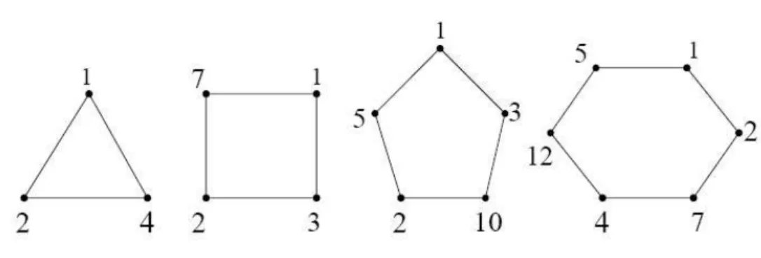
(25) since (4a2 + 7a + 2ab + 3b − 1) − (n2 + 6n − 4)/4 = a + b(6 − b)/4 ≥ a ≥ 2. For example(see Figure 11), M (P9 ) ≥ 33 in [9]. But we have M (P9 ) ≥ 36 here.. 3.2. Cycle Cn. Figure 12: Maximal IC-colorings of C3 , C4 , C5 and C6 . Let’s refer to [8], we know that M (Cn ) = n(n − 1) + 1 for n = 3, 4, 5, 6, 8, 9. And we also find M (C7 ) ≥ 39 by using computer. We also come up with a systematic way of finding an IC-coloring of Cn . Since the graph Cn has n(n − 1) + 1 connected subgraphs, M (Cn ) ≤ n(n−1)+1 by Observation 1.7. Also, Fink[3] has presented a saturating labeling of Cn with sum n(n+1)/2 as the lower bound of M (Cn ). Again, with the help of computer, we have the following improved bounds about the cycles Cn for n ≥ 10. Without loss of generality, let V (Cn ) = {v1 , v2 , · · · , vn } and let the vertices are sorted clockwise. And suppose that there exists an IC-coloring f of Cn such that S(f ) = f (v1 )+f (v2 )+· · ·+f (vn ). (1) n = 3 : M (C3 ) = 7. (2) n = 4 : M (C4 ) = 13. (3) n = 5 : M (C5 ) = 21. (4) n = 6 : M (C6 ) = 31. (5) n = 7 : 43 ≥ M (C7 ) ≥ 39 = 1 + 1 + 7 + 11 + 6 + 10 + 3 = 1 + 3 + 2 + 7 + 8 + 8 + 10 = 1 + 2 + 13 + 7 + 7 + 4 + 5 = 1 + 3 + 14 + 6 + 5 + 2 + 8 = 1 + 4 + 2 + 7 + 3 + 8 + 14 ≥ 28. Note that 43 and 28 are the known upper and lower bounds of IC-index of M (C7 ). 18.

(26) (6) n = 8 : M (C8 ) = 57 (7) n = 9 : M (C9 ) = 73 (8) n = 10 : 91 ≥ M (C10 ) ≥ 62 = 1 + 3 + 2 + 10 + 13 + 13 + 13 + 1 + 3 + 3 ≥ 10(10 + 1)/2. Note that 91 and 55 are the known upper and lower bounds of IC-index of M (C10 ). (9) n = 11 : 111 ≥ M (C11 ) ≥ 79 = 1+3+2+11+14+14+14+14+1+3+2 ≥ 11(11+1)/2. Note that 111 and 66 are the known upper and lower bounds of IC-index of M (C11 ). (10) n = 12 : 133 ≥ M (C12 ) ≥ 87 = 1 + 3 + 2 + 12 + 15 + 15 + 15 + 15 + 1 + 3 + 3 + 2 ≥ 12(12 + 1)/2. Note that 133 and 78 are the known upper and lower bounds of IC-index of M (C12 ). From the results listed above, we improve the lower bounds of IC-indices of Cn . For example, the lower bound 87 of M (C12 ) is better than 78 which is the trivial lower bound.. Figure 13: The IC-colorings of the cycle Cn. 19.

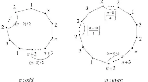
(27) Theorem 3.3. For n ≥ 10, the lower bound of M (Cn ) is : (1) If n is odd, M (Cn ) ≥ (n2 + 4n − 7)/2. (2) If n is even, M (Cn ) ≥ (n2 + n + 14)/2 + 2b(n − 9)/2c. Proof. Case 1. If n is odd, M (Cn ) ≥ (n2 + 4n − 7)/2, which is obtained by labeling V (Cn ) with 1, 3, 2, n, (n + 3), (n + 3), · · · , (n + 3), 1, 3, 2, 2, · · · , 2 in circular order, where (n + 3) repeated (n − 3)/2 times and 2 repeated (n − 9)/2 times. Case 2. If n is even, M (Cn ) ≥ (n2 + n + 14)/2 + 2b(n − 9)/2c, which is obtained by labeling V (Cn ) with 1, 3, 2, n, (n+3), (n+3), · · · , (n+3), 1, 3, 2, 2, · · · , 2, 3, 2, 2, · · · , 2 in circular order, where (n + 3) repeated (n − 4)/2 times and 2 repeated b(n − 10)/4c and b(n − 8)/4c times, respectively. We can easily check that they are satisfied with the property of IC-coloring. Hence, we have an improved lower bound of IC-coloring of cycle Cn . Though we could not decide the IC-index of Cn , we improve the lower bound of M (Cn ) which are better than the trivial lower bounds [9] : M (Cn ) ≥ n(n + 1)/2.. 20.

(28) 3.3. Double-stars DS(m, n). Review that a double-star has two central vertices plus leaves.(Figure 14 is an example.) These graphs are trees of diameter three. For convenience, we use DS(m, n) to denote a double-star whose two central vertices have degrees m and n, respectively. The following result deserved to be mentioned first.. Figure 14: Double-star DS(2, n). Lemma 3.4. [9] For 2 ≤ m ≤ n, the IC-index of DS(m, n) is at least (2m−1 +1)(2n−1 +1).. Figure 15: Lower bound of double-star DS(m, n). 21.

(29) Lemma 3.5. If f is an IC-coloring of DS(m, n), then the value of any central vertex must be the sum of some leaves. Proof. Let u and v be the only two central vertices of DS(m, n), respectively; f (u) and f (v) be the labels of them. If f (u) = a is not the sum of some leaves, then the subgraph H which satisfies fs (H) = S(f ) − a must be a disconnected subgraph since u is a cut-vertex. Vertex v is the same case. Hence, we finish the lemma. Proposition 3.6. For 2 ≤ m ≤ n, G = DS(m, n) has left and right central vertices, u and v, which are the cut-vertices, and the others are the leaves. Let L = {u1 , u2 , · · · , um−1 } and R = {v1 , v2 , · · · , vn−1 } be the set of left and right leaves, respectively. Without loss of generality, we assume f (u1 ) ≤ f (u2 ) ≤ · · · ≤ f (um−1 ) and f (v1 ) ≤ f (v2 ) ≤ · · · ≤ f (vn−1 ). If f is a maximum IC-coloring of DS(m, n), then there does not exist (1) f (uj ) = (2) f (vl ) =. P i∈{1,2,···,j−1}. f (ui ) for 1 ≤ i < j ≤ m − 1, and. k∈{1,2,···,l−1}. f (vk ) for 1 ≤ l < k ≤ n − 1.. P. Proof. (1) By Lemma 3.4, M (DS(m, n)) ≥ (2m−1 + 1)(2n−1 + 1). One can easily check that G has (2m−1 + 1)(2n−1 + 1) + m + n − 3 subgraphs. First, we consider the left leaves. If j = m − 1, and i = 1, 2, · · · , m − 2. So, P f (um−1 ) = i∈{1,2,···,m−2} f (ui ) = f (u1 ) + f (u2 ) + · · · + f (um−2 ) , then there are at least 2n−1 + 2 subgraphs of the same sums. Observe that when we choose less ui for ui ∈ {u1 , u2 , · · · , um−2 }, it produces more subgraphs of the same sums. For example, if P f (um−1 ) = i∈{1,2,···,m−2} f (ui ) = f (um−2 ), it produces 1 + 2m−3 2n subgraphs of the same sums. Hence, it reduces the known lower bound (2m−1 + 1)(2n−1 + 1) since 2 ≤ m ≤ n. Thus, f is not a maximum IC-coloring of DS(m, n). The same interpretion for j = 2, 3, · · · , m − 2 (2) The right leaves has the same result like the left ones .. 22.

(30) 3.4. Corollaries of known results. We can decide the lower bounds of certain graphs by the results of the IC-index of star ST (n) (proved by Penrice [8]) and the lower bound of the IC-index of double-star DS(m, n) (proposed by [9]). The following two corollaries were proposed by Ebrahim Salehi, Sin-Min Lee and Mahdad Khatirinejad [9], but did not give proper proofs yet. Hence, we will give the proofs of them. Then, we will have a general lower bounds of IC-index of the certain graphs. Corollary 3.7. [9] If ∆ = ∆(G) is the maximum degree of a connected graph G, then M (G) ≥ 2∆ + 2. Proof. Let u be the vertex with the maximum degree ∆ of a connected graph G. Also, we use N (u) to denote the set of the neighbors of vertex u. Hence, we have |N (u)| = ∆. Observe that the subgraph H induced by u and N (u) contains a star ST (∆). So, we get M (H) = 2∆ + 2 showed in Penrice [8]. And by Observation 1.7, we have M (G) ≥ M (H) = 2∆ + 2.. Corollary 3.8. For any triangle-free graph G with more than two vertices, we have M (G) ≥ (2∆−1 + 1)(2δ−1 + 1), where ∆ and δ denote the maximum and minimum degrees of G, respectively. Proof. Let u and v be the vertices with the maximum degree ∆ and the minimum degree δ, respectively. According to the adjacency of vertex u and v, we consider the following two cases : Case 1. u and v are adjacent : Observe the subgraph induced by the vertices set N (u). S. N (v) is the double-star. DS(∆, δ). Hence, it satisfies the inequality : M (G) ≥ (2∆−1 + 1)(2δ−1 + 1). The bound is very sharp. For example, a graph ST (n) can be viewed as a double-star DS(1, n). And they have the same IC-index 2n + 2. Case 2. u and v are not adjacent : 23.

(31) Since the vertex v with the minimum degree δ is not adjacent with the vertex u, then vertex u must be adjacent with a vertex z such that deg(z) ≥ δ. When we consider the double-star DS(∆, deg(z)), it will fit the inequality : M (G) ≥ (2∆−1 + 1)(2deg(z)−1 + 1). And since deg(z) ≥ δ, we get the inequality : M (G) ≥ (2∆−1 + 1)(2δ−1 + 1).. 3.5. Improved lower bounds of some Graphs. The IC-index of complete bipartite graph K(m, n) is not decided yet so far. But [9] has shown that for any integer n ≥ 2, the IC-index of the complete bipartite graph K(2, n) is 3 · 2n + 1. It may give some information to prove M (K(m, n)). Here, we obtain a lower bound of M (K(m, n)). Note that when m = 2, it is equal to M (K(2, n)) = 3 · 2n + 1. When m = n = 2, K(2, 2) is a C4 , and we know M (K(2, 2)) is equal to M (C4 ) = 13. Lemma 3.9. For any two integers 2 ≤ m ≤ n, the IC-index of K(m, n) is at least 1 + 2n−2 (m + 1)(m + 2). Proof. Let A and B be the two partite sets of K(m, n), where A = {u1 , u2 , · · · , um } and B = {v1 , v2 , · · · , vn }. There exists an IC-coloring f such that f (ui ) = 2i for 1 ≤ i ≤ m, and f (v1 ) = 1, f (v2 ) = 2m + 2, f (vj ) = 2j−3 α for 3 ≤ j ≤ n, where α = f (u1 ) + f (u2 ) + · · · + f (um ) + f (v2 ) = (m + 1)(m + 2). Hence, we can easily check that f is an IC-coloring. And the IC-index of K(m, n) is at least 1 + 2n−2 (m + 1)(m + 2).. Figure 16: IC-coloring of K(m, n). 24.

(32) Lemma 3.10. For any integer a ≤ b ≤ c, the IC-index of the complete tripartite K(a, b, c) is at least 2c (1 + 2b−2 (a + 1)(a + 2)). Proof. Let A, B and C be the three partite sets of K(a, b, c), where A = {u1 , u2 , · · · , ua } and B = {v1 , v2 , · · · , vb } and C = {w1 , w2 , · · · , wc }. Let f be a labeling such that f (ui ) = 2i for 1 ≤ i ≤ a, and f (v1 ) = 1, f (v2 ) = 2a + 2, f (vj ) = 2j−3 M for 3 ≤ j ≤ b, and f (wk ) = 2k−1 N for 1 ≤ k ≤ c, where M = f (u1 )+f (u2 )+· · ·+f (um )+f (v2 ) = (a+1)(a+2) and N = f (u1 ) + f (u2 ) + · · · + f (ua ) + f (v1 ) + f (v2 ) + · · · + f (vb ) = 1 + 2b−2 (a + 1)(a + 2). Hence, we can easily check that f is an IC-coloring. And the IC-index of the complete tripartite M (K(a, b, c)) is at least 2c (1 + 2b−2 (a + 1)(a + 2)).. Figure 17: IC-coloring of the complete tripartite K(a, b, c). Proposition 3.11. For any integer m1 ≤ m2 ≤ · · · ≤ mn , the IC-index of the complete multipartite K(m1 , m2 , · · · , mn ) is at least 2mn 2mn−1 · · · 2m3 (1 + 2m2 −2 (m1 + 1)(m1 + 2)).. 25.

(33) Wheels with n spokes, denoted by Wn , are obtained by the join operator Cn +K1 . It is shown that the IC-index of Wn satisfies the following inequalities [9] : 2n + 2 ≤ M (Wn ) ≤ 2n + n(n − 1) + 1 for n ≥ 3. Here, we have an improved lower bound of Wn . Theorem 3.12. For any integer n ≥ 3, M (Wn ) ≥ 2n + 5. Proof. Observe that if n = 3, W3 is K4 . Hence, M (W3 ) is equal to 15, which fits the upper bound of M (Wn ) tightly. Thus, we consider the case when n ≥ 4. Let V (Wn ) = {v0 , v1 , v2 , · · · , vn } for n ≥ 4. Let v0 be the central vertex, and vertices v1 , v2 , · · · , vn are ordered clockwise. Then there exists an IC-coloring f such that f (v0 ) = 6, f (v1 ) = 2, f (v2 ) = 1 and f (vi ) = 2i−1 for 3 ≤ i ≤ n. Thus, we can easily check that f is an IC-coloring, and the IC-index of Wn is at least 2n + 5. Note that when n = 3, W3 is K4 . So M (W3 ) = 24 − 1 = 15, which fits the upper bound 2n + n(n − 1) + 1. But we have M (W4 ) ≥ 27, M (W5 ) ≥ 46, and M (W6 ) ≥ 76, which are the better lower bounds than the results obtained in [9] and Theorem 3.12. Note that the values of central vertices of Wn for n ≤ 6 are different from that of central vertices of Wn when n ≥ 7.. Figure 18: The central labels are 1 when n ≤ 6 and 6 when n ≥ 7.. 26.

(34) 4. Conclusion. From the study of the Stamp Problem, we have noticed that the most difficulty part of obtaining M (G), the IC-index, is knowing the exact upper bound. Even we can figure out the number of distinct connected subgraphs of G, we have no idea whether some distinct connected subgraphs will come out with the same value from a labeling due to the structure of the graph G. Double-star is one of such graphs. So, to determine the IC-index of a general graph is not going to be an easy work. It’s left a lot of works to do. But, certainly, we should be able to do a better job in the near future after knowing more inside of this topic.. 27.

(35) References [1] R. Alter and J. A. Barnett, A postage stamp problem, Amer. Math. monthly 87(1980), 206-210. [2] B. Bolt, Mathematical Cavalcade, Cambridge University Press, Cambridge, 1992. [3] J. F. Fink, Labelings that realize connected subgraphs of all conceivable values, Congressus Numerantium 132 (1998), 29-37. [4] J. A. Gallian, A survey : recent results, conjectures, and open problems in labeling graphs, J. Graph Theory 13 (1989), 491-504. [5] R. Guy, The postage Stamp Problem, Unsolved Problems in Number Theory, second ed., Springer, New York 1994, 123-127. [6] R. L. Heimer and H. Langenbach, The Stamp Problem, J. Recreational Math. 7 (1974), 235-250. [7] W. F. Lunnon, A postage stamp problem, Comput. J. 12 (1969), 377-380. [8] S. G. Penrice, Some new graph labeling problems: a preliminary report, DIMACS Tech. Rep. 95-26m (1995), 1-9. [9] E. Salehi, Sin-Min Lee and M. Khatirinejad, IC-Colorings and IC-Indices of graphs, Discrete Mathematics 299 (2005), 297-310. [10] Douglas. B. West (2001), Introduction to graph theory, Upper Saddle River, NJ : Prentice Hall.. 28.

(36)