全域性無線數位家庭多媒體網路管理

(1)

行政院國家科學委員會專題研究計畫成果報告

全域性無線數位家庭多媒體網路管理

計畫類別：個別型計畫

計畫編號： NSC94-2213-E-004-011-

執行期間： 94 年 08 月 01 日至 95 年 07 月 31 日

執行單位：國立政治大學資訊科學系

計畫主持人：蔡子傑

計畫參與人員：蔡子傑、江啟宏、&#63969；政霖、&#63988；建圻、張碩瀚、

王川耘、&#63943；姿吟

報告類型：精簡報告

報告附件：出席國際會議研究心得報告及發表論文

處理方式：本計畫可公開查詢

中華民國 95 年 10 月 18 日

(2)

行政院國家科學委員會補助專題研究計畫成果報告

全域性無線數位家庭多媒體網路管理

計畫類別：■ 個別型計畫 □ 整合型計畫

計畫編號：NSC 94－2213－E－004－011

執行期間： 94 年 8 月 1 日至 95 年 7 月 31 日

計畫主持人：蔡子傑

共同主持人：

計畫參與人員：江啟宏、李政霖、林建圻、張碩瀚、王川耘、劉姿吟

成果報告類型(依經費核定清單規定繳交)：■精簡報告 □完整報告

本成果報告包括以下應繳交之附件：

□赴國外出差或研習心得報告一份

□赴大陸地區出差或研習心得報告一份

■出席國際學術會議心得報告及發表之論文各一份

□國際合作研究計畫國外研究報告書一份

處理方式：除產學合作研究計畫、提升產業技術及人才培育研究計畫、

列管計畫及下列情形者外，得立即公開查詢

□涉及專利或其他智慧財產權，□一年□二年後可公開查詢

執行單位：國立政治大學資訊科學系

中華民國 95 年 10 月 17 日

(3)

行政院國家科學委員會專題研究計畫成果報告

全域性無線數位家庭多媒體網路管理

計畫編號：NSC 94-2213-E-004-011

執行期限：94 年 8 月 1 日至 95 年 7 月 31 日

主持人：蔡子傑國立政治大學資訊科學系

計畫參與人員：江啟宏、李政霖、林建圻、張碩瀚、王川

耘、劉姿吟

此成果報告為五篇論文的集節：

[1] Tzu-Chieh Tsai, Cheng-Lin Li, Tsung-Ming Lin, "Reducing Calibration Effort for WLAN Location and Tracking System using Segment Technique" in The IEEE International Workshop on Ad Hoc and Ubiquitous Computing (AHUC2006), Taichung, T a i w a n , J u n e 5 - 7 , 2 0 0 6 . [2] Tzu-Chieh Tsai, Tzu-Yin Liu, "Bandwidth Routing Support for Wireless Multihop Networks", in IEE Mobility Conference 2005: The Second International Conference on Mobile Technology, Applications and Systems, Nov 15-17, 2005, G u a n g z h o u , C h i n a . ( E I ) [3] Tsai Tzu-Chieh, Lin Chien-Chi, "Efficient Routing Path Selection Algorithm based on Pricing Mechanism in Ad Hoc Networks", in International Computer Symposium (ICS 2006), Taipei, Taiwan, D e c 0 4 - 0 6 , 2 0 0 6 . [4] Chi-Hong Jiang, and Tzu-Chieh Tsai, "Token Bucket Based CAC and Packet Scheduling for I E E E 8 0 2 . 1 6 B r o a d b a n d W i r e l e s s A c c e s s Networks", in IEEE Consumer Communications and Networking Conference 2006 (CCNC2006), Special Session on Multimedia and QoS in Wireless Networks, MP1-02-3, Jan 8-10, 2006, Las Vegas,

U S A .

[5] Tzu-Chieh Tsai, Sol-Han Chang, “The Streaming Service Platform based on EATCP for Heterogeneous Wireless networks”, submitted to IEEE Wireless Communications & Networking Conference (WCNC 2007), Hong Kong, Mar 11-15,

2 0 0 7 . 首先我們先整理摘錄此五篇論文在本計畫中的關聯度與重要成果，後附上完整論文內容供參考。其中第五篇在審查中，基於智慧財產權，暫不附全文，請見諒。一、Abstract 近年來數位家庭與無線網路硬體技術的逐漸發展，使得建置一個smart home environment 的願景

逐步呈現。這樣一個環境必須能夠感知個人情境，隨時隨地能透過周邊的智慧型數位家電，擷取多媒體個人資訊，並隨著行動過程，藉由週遭感知設備，自主追蹤及定位相關個人或數位家電位置，而能提供具一定服務品質的資訊遞送。

我們假設家中有一個 Media & Network server來統一控管整個家的網路環境設備與系統。使用UPnP(Universal Plug and Play)的概念，讓所有的intelligent devices一旦啟動之後，便會自動接合上整個智慧型家庭環境網路，並同時向 Media & Network server註冊。在資料傳輸的協定上，在室內，我們使用IEEE 802.11無線區域網路提供穩定的網路服務品質；在室外WLAN無法涵蓋的區域，則是需要涵蓋範圍較大的802.16都會型區域網路來加強WLAN涵蓋範圍不足的缺陷。本研究的主要目的，是希望由網路的各種技術為基礎，提供一個完整而具前瞻性的新數位家庭生活環境，並透過中央的Media & Network server來對整個家庭成員及設備作一整體性的管理，以期對人類的生活作突破性的進步。我們研究的主要關鍵技術將包括:（1）室內無線定位暨追蹤預測技術，（2）WLAN 與 Mobile Ad hoc Networks 的具服務品質的通訊協定改良，（3）即時性多媒體串流應用的遞送品質

(4)

Keywords: 自主定位追蹤、 Mobile Ad Hoc Networks、網路服務品質、智慧型家庭、多媒體串流應用 二、緣由與目的、結果與討論 在數位家庭的成員中攜帶著各式各樣的行動裝置，特別是多媒體或具上網能力的裝置，我們希望家中的 Media & Network Server，可以隨時隨地掌控到他們的位置，如此才方便管理網路的資源配置，與內容的遞送與交替，達到智慧型家庭的體貼式的服務。因此，這個部份我們研究了利用 IEEE 802.11 RF 的特性，來分析與實作出定位系統，成果為論文[1]。其次無線區域網路在佈建數位家庭可能含蓋率會有所不足，既然家電視聽設備都有網路介面，因此自然可以形成多跳接隨意型網路，以增加其彈性與無線網路含蓋率，並降低佈建成本。但是，也衍生出管理與控制問題，如何有效管理與維持一定服務品質與效能就是成果報名論文[2][3]的內容。如果採用 802.16 網路來增加 WiFi 含蓋率不足的話，怎樣來管理多媒體應用的服務分級，是成果報告論文[4]。最後，在異質性網路的多媒體遞送的協定研究，則是論文[5]。

1. "Reducing Calibration Effort for WLAN Location

and Tracking System using Segment Technique" 1.1 Abstract

As mobile computing technology becomes more and more mature, people feel great interest on context-aware applications and services. Referring to context, location-aware system is one of the most important components. This paper presents a precise indoor RF-based (IEEE 802.11) locating system named Precise Indoor Locating System (PILS). In order to acquire high level of location estimation result, a large number of training samples should be collected in offline phase. As a result, the system becomes impractical and huge number of man-power is needed. In this paper, we aim to reduce the manual effort in constructing radio map and maintain high accuracy in our system. We propose models for data calibration, interpolating, location estimation, and tracking in PILS. Wireless Channel Propagation model is also in our concern. Large scale and small scale fading are involved in the wireless channel propagation.

1.2 Main Results

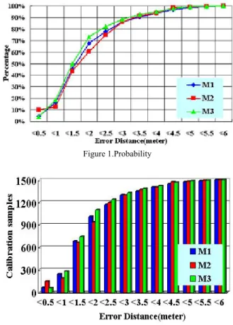
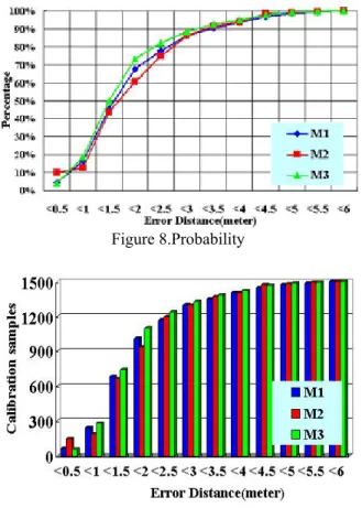
In figure 1 and figure 2, the calibrated point rate is 9.7%, and data of other grid points are interpolated.

We integrate all experiments data in these two figures. As we can see, Figure 1 shows the accuracy probability on each model and figure 2 illustrates the accuracy distribution. In figure 1, M3 owns the highest probability when error distance is within 2 meters, and it reaches about 73.40%. M1 performs better than M2 within 2 meters of error distances and they all exceed 60% on 2 meters. Figure 2 illustrates the distribution of all 1500 experiment samples. Within 2 meters of error distances, 1101 samples are eligible in M3, 935 samples in M2, and 1013 in M1. The result shows high accuracy since the calibrated point rate is 9.7%.

In figure 3 we compare our models with well-known WLAN location system RADAR which is designed by Microsoft. Two experiments were held, one calibrated data on 9.7% greed points and calculated the rest 90.3%, and the other calibrated data on 100% points. The result shows that average error distances in our model are 1.5968 m with 9.7% points and 0.9076 m with 100% points. The average error distances in RADAR are 2.4368 m with 9.7% points and 1.7588 m with 100% points. It’s obvious that our system owns better location estimation result than RADAR because more information are acquired with the Segment Process and novel location estimation models are presented by us.

Figure 1.Probability

(5)

Figure 3.Comparison between (M1+M2) and RADAR

2. "Bandwidth Routing Support for Wireless

Multihop Networks" 2.1 Abstract

The idea of mobile computing service is to provide a ubiquitous information environment. However, the present mobile ad hoc networks still can’t support real-time transmission very effectively. In other words, the capability of supporting QoS guarantee has become a very important issue. IEEE 802.11 PCF adopts the polling scheme to provide time-bounded traffic services, which is not suitable in multi-hop networks. Moreover, due to mobility and traffic dynamics, the network resource management is more difficult. Thus, QoS support in such an environment is a challenge. Specifically, path bandwidth calculation is the first key element. All the bandwidth routing papers we referred to were using TDMA. However, they are restricted in TDMA systems and somehow complicated in path bandwidth calculation. We propose a simple path bandwidth calculation solution that can be used for any kinds of MAC protocols. It is also easy to implement call admission control and to combine with bandwidth routing algorithms. The simulation results illustrate that the statistical error rates of our path bandwidth calculation are within an acceptable range. By path bandwidth calculation, bandwidth routing algorithm is also developed to achieve the objective of supporting QoS in wireless multihop networks effectively.

2.2 Main Results

We the maximal available remaining bandwidth between the estimation and real network traffic through the throughput information we obtained. Fig. 4 depicts the comparison of CBR and VBR traffic.

Fig. 4. Available Bandwidth Comparison

Finally, we evaluate our bandwidth calculation in a more typical wireless multi-hop topology as shown in Fig. 5.

Fig. 5. Integrated Scenario

Fig. 6 is the simulation result that depicts the average achieved throughput ratio. The ATR decreases slightly while the background traffic loading increases. Overall, the average ATR are acceptable which are almost above 85%. Although there exists statistical inaccuracy in our solution, our proposed estimate still get stable results even we ignore the IEEE 802.11 MAC overhead.

Fig. 6. Average Achieved Throughput Ratio

Fig. 7 shows the normalized delay time of the simulation. The mean normalized delay time jumps with the increase of traffic load. The VBR traffic delay time ascends more obviously than CBR traffic delay time when traffic load is high. This result might be caused by IEEE 802.11 overhead or our inaccuracy.

(6)

Fig. 7. Mean Normalized Delay Time

3. "Efficient Routing Path Selection Algorithm based

on Pricing Mechanism in Ad Hoc Networks" 3.1 Abstract

In military and rescue applications of mobile ad hoc networks, all the nodes belong to the same authority； therefore, they are motivated to cooperate in order to support the basic functions of the network. However, the nodes are not willing to forward packets for the benefit of other nodes in civilian applications on mobile ad hoc networks. In this research, we adopt the “pay for service” model of cooperation, and propose a pricing mechanism combined with routing protocol. The scheme considers user’s benefits and interference effect in wireless network, and can distribute traffic load averagely to improve network performance. The simulation results show that our algorithm outperforms than other routing protocols.

3.2 Main Results

In this section, we present the simulation results and analysis. AOP-L is the method which chooses the longest expected connection time from efficient routing paths. AOP-P is the method which chooses the lowest price from efficient routing paths.

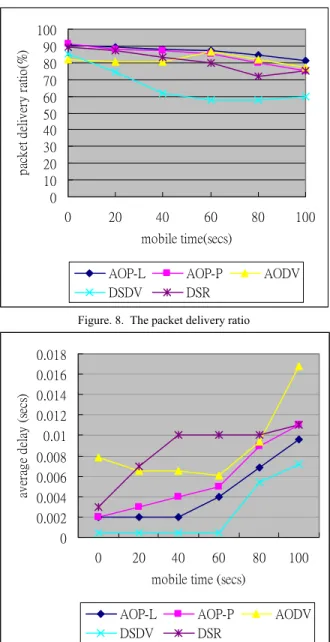
From figure 8 we can find that on-demand routing protocols delivery over 70% of the data packets regardless of mobility rate, and outperform the table-driven routing protocol, DSDV.

Figure 9 shows the average end to end delay. The average end-to-end delay of packet delivery is lower in AOP-L and AOP-P as compared to other on-demand routing protocols.

From figure 10 we can find AOP-L and AOP-P are more efficient than other routing protocols. Using AOP routing protocol, users can transfer packets with the less payment. 0 10 20 30 40 50 60 70 80 90 100 0 20 40 60 80 100 mobile time(secs) pa ck et d el iv er y ra tio( % )

AOP-L AOP-P AODV DSDV DSR

Figure. 8. The packet delivery ratio

0 0.002 0.004 0.006 0.008 0.01 0.012 0.014 0.016 0.018 0 20 40 60 80 100 mobile time (secs)

av er ag e de la y (s ec s)

(7)

0 1 2 3 4 5 6 7 8 9 10 0 20 40 60 80 100

mobile time (secs)

PD

R * 1

00 / p

ayme

nt

Figure. 10. Efficiency

The simulation results bring out some important characteristic differences between the routing protocols. The presence of high mobility implies frequent link failures and each routing protocol reacts differently during link failures. The different basic working mechanisms of these protocols lead to the differences in the performance. The results show that our routing protocols (AOP-L and AOP-P) outperform than other routing protocols. Although the packet delivery of AOP is almost the same with others, the end-to-end delay is lower and the efficiency is highest.

4. "Token Bucket Based CAC and Packet Scheduling

for IEEE 802.16 Broadband Wireless Access Networks"

4.1 Abstract

The IEEE 802.16 standard was designed for Wireless Metropolitan Area Network (WMAN). It supports QoS and has very high transmission rate. The key part of 802.16 – packet scheduling, was undefined and is an open issue. We first proposed a token-bucket based uplink packet scheduling combined with call admission control (CAC) of 802.16. Then a model of characterizing traffic flows by token bucket is presented. The simulation results show that our CAC and uplink packet scheduling can promise the delay requirement of rtPS flows and our model can predict the delay and loss of a traffic flow precisely.

4.2 Main Results

We show the simulation results for CAC and uplink packet scheduling.

Two methods of CAC and uplink packet scheduling are compared here. Method 2 was proposed in the

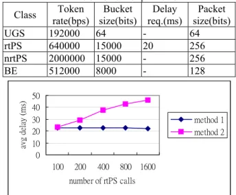
literature and method 1 was proposed by us. The parameters of four classes are listed in Table 1.

The begin time of each flow is Poisson distribution. All flows send data during each frame in full speed. Frame duration f is 1ms and simulation time is 150ms.

Table 1. Simulation parameters

Class _rate(bps)Token _size(bits)Bucket _req.(ms)Delay _size(bits)Packet UGS 192000 64 - 64 rtPS 640000 15000 20 256 nrtPS 2000000 15000 - 256 BE 512000 8000 - 128 0 10 20 30 40 50 100 200 400 800 1600 number of rtPS calls avg de la y (ms) method 1 method 2

Figure 11. Average delay v.s. number of rtPS calls

From Figure 11 we can find that the average delay of rtPS used by our method is almost constant no matter how many rtPS calls exist.

5. “The Streaming Service Platform based on EATCP for Heterogeneous Wireless networks”

5.1 Abstract

With the growth of broadband access networks, the demand of streaming service increased. In tradition, UDP is the only option for streaming service. UDP will suffer the various losses in heterogeneous wireless network. In our work, we develop an Error-Adaptive TCP for the purpose of streaming service in heterogeneous wireless network. EATCP-Assisted Module could collect the information of MAC layer such as wirelessRTT, and Link utilization. After the sender receive the information that from MAC layer and from itself, it can estimate the wiredBW and wirelessBW. Based on the estimation the sender adjusts the congestion window in a proper heuristic manner. EATCP could also adjust the congestion window based on the bandwidth demand of application. Under the help of simulator, we will prove the EATCP could have better performance under heterogeneous wireless networks.

5.2 Main Results

Fig.12 shows the total throughput. In this kind of Scenario, our total throughput is a little bit higher than

(8)

other versions of TCP. Fig.13 shows the average delay of the topology, as the Figure shows our average delay is lower than other versions of TCP. The reason is that our congestion control mechanism can adjust the congestion window accordingly.

Total throughput 1000 1100 1200 1300 1400 1500 2 3 5 10 20 number of flow throughput KBps EATCP Reno Newreno Vegas JTCP

Fig 12. Total Throughput Delay 0.0135 0.014 0.0145 0.015 0.0155 0.016 2 3 5 10 20 number of flow Delay (sec) EATCP Reno Newreno Vegas JTCP

Fig 13. Average Delay

Fig 14 presents the result of the streaming service platform build on UDP or EATCP. After transmission over heterogeneous wireless networks, we will

compute the average PSNR of two films. The PSNR of two films has shown in Fig.14.

AVGPSNR 0 10 20 30 40 0 0.1 0.2 0.3 0.4 0.5 lost rate psnr (db) udp EATCP

Fig. 14. PSNR of Streaming service

三、計畫成果自評本計畫原先提出為三年期整合型計畫之子計畫之一。原本第三年要將整個系統實作作整合與展示，但可惜整合型計畫總計畫未獲推薦，所以被拆成個別型計畫，而且未有預核。因此，我們只好實作個別系統，待未來計畫再作完整整合。即便如此，我們有實際的定位系統可供進一步技轉或申請專利，同樣地 MANET QoS 管理與繞路法則，以及 WiMAX、EATCP 雖沒有實作系統，不過也可考慮技轉或專利。未來無線數位家庭的建置，如果有這些模組的整合，相信一定可以作到全域性且智慧型的無線多媒體網路管理。這也就是這篇報告最大的貢獻。

(9)

Reducing Calibration Effort for WLAN Location and Tracking System using

Segment Technique

Tzu-Chieh Tsai, Cheng-Lin Li, Tsung-Ming Lin

Department of Computer Science

National Cheng Chi University

Taipei, Taiwan

{ttsai, g9303, s9109}@cs.nccu.edu.tw

Abstract

As mobile computing technology becomes more and more mature, people feel great interest on context-aware applications and services. Referring to context, location-aware system is one of the most important components. This paper presents a precise indoor RF-based (IEEE 802.11) locating system named Precise Indoor Locating System (PILS). In order to acquire high level of location estimation result, a large number of training samples should be collected in offline phase. As a result, the system becomes impractical and huge number of man-power is needed. In this paper, we aim to reduce the manual effort in constructing radio map and maintain high accuracy in our system. We propose models for data calibration, interpolating, location estimation, and tracking in PILS. Wireless Channel Propagation model is also in our concern. Large scale and small scale fading are involved in the wireless channel propagation.

1. Introduction

In wireless network research, context-aware applications and mobile computing are interested by investigators in recent years. To establish an intelligent environment with context-aware applications is significant for human life. A key feature of context-aware applications and mobile computing is the location information. Via location information, a number of geographical and commercial applications are derived. For example, the museum guiding system does.

It’s critical to develop a locating system indoors with high accuracy. Several studies have been conducted to offer some locating theorems. Many of above implement based on signal strength(SS) and access point(AP) information and supply a model for

their location calculation. Although regarding signal strength is somehow sufficiently to obtain location of mobile terminal with low deviation, it’s more workable to consider with physical architecture property. Real world wireless channel can be decomposed into two parts: large-scale model and small-scale fading model. Large-scale model considers the path loss which represents the local mean of the channel gain and is therefore dependent on the distance between the transmitter and receiver. Small-scale fading is a characteristic of radio propagation resulting from the presence reflectors and scatters that cause multiple versions of the transmitted signal to arrive at the receiver, each distorted in amplitude, phase and angle of arrival.

Most RF-based location systems are operated in two phases: offline calibration phase and online estimation phase. In offline calibration phase, location system calibrates a great deal of data on specific location and stores these data which is labeled with location information into database, which is called radio map. In online estimation phase, system calibrates some data in real time and substitutes them into radio map for estimating people’s location. The greater part of RF-based location system described above demand large amount of calibration data. It’s manpower-wasted to calibrate a lot of data for each building. Reducing offline calibration effort and making estimation result acceptable are our goals in this paper. We expect to train data on one location in small room and to train less than three locations in bigger ones.

We propose a methodology called Segment Process. Both offline and online phases refer to the concept of Segment Process. In offline phase we use Segment Process to gain more useful data in radio map, and in online we use it for making estimation result more accurate. Segment Process only consumes computer calculation frequency but needn’t more manual effort. The detail of Segment Process will introduce below.

(10)

The result of PILS is very useful regarding context-aware applications. PILS is able to evaluate mobile terminals’ location within few meters to their actual location. It’s also remarkable that PILS decreases large amount of manual effort when calibrating data. PILS is more practical than other location system and is with fine estimation accuracy.

The remainder of this paper is organized as follows. In Section 3, we lay out our concept in estimating user’s location and present our locating system in Section 4. Experiment results are described in Section 5. In Section6, we summarized the conclusion of this paper.

2. Location Estimation Concept

2.1 Segment Process

Figure 1.Segment Process

As described above, wireless channel signal strengths are changeful. Even immovable calibrating, the signal strengths still pulse up and down. Inconstant signal strengths on one position make estimating location difficult and inaccurate. Most research adopts mean value to solve this problem, but we think it’s insufficient through inexact location estimating result. Using one mean value to stand for one position’s wireless channel information is not enough. We present a Segment Process to make some improvement.

Assume one training process gains 100 signal strengths, we divide up these 100 signal strengths into 10 parts, each has 10 signal strengths. Then calculate mean value of each part and store them into radio map to substitute for original one mean value. Now we acquire 10 slices of mean values and have more information to estimate location. We call the divide procedure as Segment Process. Not only in offline calibration phase we do Segment Process, but in online estimation phase we execute it, as will introduce below.

In our opinion, mean value is used for expressing proper wireless channel characteristic. Using Segment Process to obtain more slices of mean values denotes more information to refer to and more accurate location estimation result.

2.2 Reducing Training Location Numbers

A lot of proposed research show high accuracy of location estimation. But they are all unpractical due to high manual effort. We are incapable to train radio map for all buildings with high manual effort. Construct a location system that only requires little offline training effort is significant. These kinds of methods are called reducing calibration effort. Recent research which achieve high accuracy within 1 meter error distance calibrate data on all grid points. In our model we train data on one grid point in small room and within three grid points in bigger one, and then interpolate data for all the other grid points. We will describe it in section 3.3.

2.3 Reducing Calibration Time

Reducing calibration time is one of the methods to decrease manual effort. In recent years, most research with high accuracy calibrate large amount of data on fixed location. It normally requires tens or even hundreds of samples to stabilize signal strength distributions. With constant calibration frequency, the ratio between calibration samples and time is linear. Therefore, reducing calibration time to half of the origin means that only 50% of samples can be collected. Our experiments shows that amount of calibration samples can be reduced to 50% and the accuracy could be maintained above 80%. As a consequence, decreasing calibration time descends the manual effort and makes the system more practical.

3. Location Estimation Model

3.1

Variable Definitions

Assume in one calibration we gain n data, and detect i APs. Let bi be ith AP, ssi be signal strengths

received from bi.

Si = {(ss1,bi),(ss2,bi),(ss3,bi),…,(ssn,bi)}.

Assume there are j positions in radio map. Let lj be jth

location.

Xj = {(S1,lj),(S2,lj) ,(S3,lj),…,(Si,lj)}.

We use Segment Process to divide up n data into m parts, then we get mean, 2nd_{moment, and variance for}

each part. Μij={(µi1,Xj),(µi2,Xj),(µi3, ,Xj),…,(µim,Xj)}, Μ2 ij={(µ2i1,Xj),(µ2i2,Xj),(µ2i3,Xj),…,(µ2im,Xj)}, Σij={(σi1,Xj),(σi2,Xj),(σi3,Xj),…, (σim,Xj)}. 3.2 Probability Model

As small-scale fading investigates signal fluctuation in short period of time, our Segment Process divide

(11)

calibration into small pieces of time. Definitely Segment Process matches the claim of small-scale fading. Therefore, we adopt Rayleigh-like fading probability density function as our probability model. Let Probability Model be

⎪⎭ ⎪ ⎬ ⎫ ⎪⎩ ⎪ ⎨ ⎧ Μ Μ Μ = m ij 2 2 ij 2 1 ij 2 ) ) | , ( ( ,..., ) ) | , ( ( , ) ) | , ( ( ) | ( N X S R N X S R N X S R X S P i j i j i j j i (1) where

0 S

},

2 S

exp{

S

)

X

|

,

S

(

_i ij 2 2 i ij 2 i j ij 2 i

Μ

=

_Μ

×

−

_Μ

≥

R

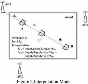
(2) 3.3 Interpolation Model

For reducing calibration number of locations, most of the data of grid points on the radio map are gained by interpolating. Large-scale fading represents the relationship between path loss and signal attenuation. Equation 3 and 4 are our interpolating models and we use them to calculate data for un-calibrated grid points on radio map. An illustration is shown in figure 2, location A and B have been calibrated and location C need to be calculated. When only location A is observable to location C, we use equation 3 to infer signal strength on location C, and when both location A and B are visible, we use equation 4. All the other un-calibrating grid points are computed with the same way. Ai Ci

S

d

S

×

+

=

)

(

log

1 0 0 (3) Bi Ai Ci

_d

S

d

S

d

S

×

+

×

+

=

)

(

log

)

(

log

2 1 1 2 1 2 (4)

Once we calculate all the signal strengths of un-calibrated grid points on radio map, we use Segment Process to divide data of each point into m parts. Meanwhile, system computes mean, second moment, variance value for each location and substitutes these values into probability model. All the details have been introduced above. After interpolating step, we establish a complete radio map for location system.

Figure 2.Interpolation Model

3.4 Location Deterministic Model 3.4.1 Pre-operation

In location deterministic model, location system estimates locations of mobile devices. We make use of Segment Process to improve the accuracy of estimation results. Assume system produces one estimation consequence every time period t. Now we separate t into m portions, and then calculate one brief result for each portion. Finally, we combine these m brief results for ultimate outcome. After pre-operation, we propose two location methodologies, which will introduce below.

3.4.2 Weighted Triangulation Model

After combining m brief results, system produces a sequence of P(Si | Xj), which form the radio map. The

radio map is defined as following:

} ) X , P(S ..., ), X , P(S ), X , P(S { )} P(X ,..., ) P(X ), {P(X RM j a i 1 a 2 a i 1 a 1 a i 1 a j 2 1 = = = Π Π Π = = (5)

Let k/m probability radio map(t=k*m, k=1,2,3…) be RMk/m. Then we multiply all RMk/m as following:

∏

= ≤ ≤ = m 1 k/m,1 k t k final RM RM (6)

Finally take the max P(Si|Xj) of RMfinal as the output

result.

Then we choose three locations XA, XB, XC, which

own the max probability values, and use weighted triangulation to determine the outcoming location. Figure 3 illustrates weighted triangulation. Being normalized, PA equals to 0.5, PB equals to 0.3, PC

(12)

equals to 0.2. As a consequence, the order of distance to estimation location from far to near is C,B,A, respectively. The equations are as follows:

C B A C C B B A A P P P P X P X P X x + + × + × + × = (7) C B A C C B B A A P P P P Y P Y P Y y + + × + × + × = (8)

Figure 3.weighted triangulation

3.4.3 Time Correlation-based Model

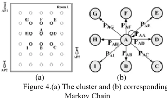
The location system is more appropriately to be implemented on the dynamic environment. We consider referring the correlation between locations. For one estimation, we form a cluster which consists with eight gird points surrounding the prior location and calculate correlation between prior location and all the other grid points in the cluster. The cluster is shown as figure 4(a), and corresponding Markov Chain is illustrated as figure 5(b).

(a) (b)

Figure 4.(a) The cluster and (b) corresponding Markov Chain

As presenting in section 3.4.1, we use Segment Process to divide one estimation into m slices of brief results and combine them for ultimate output. In all

brief calculation, system computes the correlation between prior estimation result and other gird points in the cluster. As figure 4(b) showing, assume prior result is location A, then PAA, PAB,…, PAI are calculated. Let

prior result, state A be πk_{, π}k _{= P(X}

A) = Πia=1P(Sa,XA).

Let all grid points in cluster be πk+1_{, (P}

AA,PAB ,…, PAI)

be state transition probability distribution A.

k 1 k

_A

_π

π

+

=

η πk m 1 k max arg output ₌ Π= , η is a normalizer 3.5 Tracking Model

User tracking is another issue in indoor technology. We try to analyze user’s heuristic orbit for predicting his next step. In logical thinking, the average walking velocity of human beings is 1.36 m/s. In PILS, system will record user’s locations that have passed. Then calculate his next location with these heuristic paths and judge the conformity of human average velocity.

In our tracking model, the concept of time flow is considered. When system behaves tracking, continuous calculations is operated and fore-computing is performed. With a sequence of heuristic paths, we use time correlation-based location model introduced in section 3.4.3 to implement user tracking. As imagining, a sequence of Markov Chain will be exercised. Since correlation of estimation results of each time t are calculated, we make system fore-computing twice, and backward verify the result which will be outputted.

4. Experimental Evaluation

In this section we discuss the experimental testbed and evaluate the performance of PILS with all the models in this paper.

4.1 Testbed

We performed our experiment in the second floor of the Dept of CS, National Cheng-Chi University. This building has a dimension of 11 × 52 meters. The building is equipped with 802.11b wireless LAN environment. Our experiment devices are IBM X21, six PCI GW-APIIT and six BLW-04G APs. To form the radio map, the environment was modeled as a space of 235 locations, 215 locations inside the rooms and 20 along the corridors, each representing a 1.5×1.5 meter square grid cell.

(13)

4.2 Data Collection

Since we deem that train data on too many locations on offline phase is impractical, we attempt to calibrate in few locations and interpolate all the other data on grid points by our model. In our experiment environment, we collected 1 point in small rooms, 2 points in bigger ones, and 2 points in corridor. Totally, we selected 23 locations, 9.7% in whole environment locations. On the other hand, system calculates 90.3% locations. In our opinion, newly computer owns high performance and can sustain vast data calculation. Figure

We collected 30 samples at each calibrating locations and expected an error of about 10~15 cm due to the inaccuracies when clicking the radio map.

4.3 Experimental Result

Figure 5.Performance at calibrated and interpolated locations with varying sampling data(M1) Define M1 as weighted triangulation model, M2 as time correlation-based model, and M3 as M1+M2. Figure 5 illustrates the effect of reducing the number of calibrated locations. And it also shows the factor of reducing the calibrated data on each point. The X axis represents number of training samples at one location, and the Y axis shows the accuracy whose probability of error distance is within 2 meters.

For a fixed number of training samples, for example 30 data, three measurements were held. The first experiment was taken at calibrated position, whose signal strength distributions were calculated directly from the sampled data. The second experiment was measured at interpolated positions, whose distributions were interpolated from the calibrated locations. The last one was taken at locations which are combined calibrated locations with interpolated ones. As we can see, experiments held at calibrated locations achieve best consequence. It proves that experiments with real

data produce better result. Experiments taken at overall locations own second results and have worst outputs at interpolated locations.

Figure 6 and 7 illustrate the same idea with figure 5, but they are different at that figure 5 operates with M1, and figure 6 and 7 operate with M2 and M3. We analysis these three figures together. In general, M3 has the best performance, and M2 is worst. M1 is better than M2 and worse than M3.

Figure 6.Performance at calibrated and interpolated locations with varying sampling data(M2)

Figure 7.Performance at calibrated and interpolated locations with varying sampling data(M3) In figure 8 and figure 9, the calibrated point rate is 9.7%, and data of other grid points are interpolated. We integrate all experiments data in these two figures. As we can see, Figure 8 shows the accuracy probability on each model and figure 9 illustrates the accuracy distribution. In figure 8, M3 owns the highest probability when error distance is within 2 meters, and it reaches about 73.40%. M1 performs better than M2 within 2 meters of error distances and they all exceed 60% on 2 meters. Figure 9 illustrates the distribution of all 1500 experiment samples. Within 2 meters of error distances, 1101 samples are eligible in M3, 935 samples in M2, and 1013 in M1. The result shows high accuracy since the calibrated point rate is 9.7%.

(14)

In figure 10 we compare our models with well-known WLAN location system RADAR which is designed by Microsoft. Two experiments were held, one calibrated data on 9.7% greed points and calculated the rest 90.3%, and the other calibrated data on 100% points. The result shows that average error distances in our model are 1.5968 m with 9.7% points and 0.9076 m with 100% points. The average error distances in RADAR are 2.4368 m with 9.7% points and 1.7588 m with 100% points. It’s obvious that our system owns better location estimation result than RADAR because more information are acquired with the Segment Process and novel location estimation models are presented by us.

5. Conclusions

In this paper, we proposed our RF-based WLAN location and tracking system named PILS. We analyze the variations of wireless channel propagation and develop models to solve them. Most variations of wireless channel propagation are caused by wireless channel fading which can be categorized into large-scale fading and small-large-scale fading.

Figure 8.Probability

Figure 9.Distribution

The main idea of this paper is to reduce the calibration effort and keeps the result won’t decline too much. We proposed a methodology called Segment Process. Both offline and online phases refer to the concept of Segment Process. In location deterministic model, we proposed weighted triangulation model and time correlation-based model. In online phase, weighted triangulation model chooses three deterministic locations which own higher probabilities and triangulate them for final output. Time correlation-based model considers the correlation of former output location for each determination and a Markov Chain is operated for calculating the correlation. We had taken a lot of experiments for each model and combination of them. Details of experiments are shown in section 4.3, and the result is well enough for constructing a really impractical location deterministic system.

Finally we compare our system with famed location system RADAR and demonstrate that better accuracy is presented by our system.

Figure 10.Comparison between (M1+M2) and RADAR

6. Related Work

To date, a lot of research has made effort in determining and tracking user location. Location and tracking methodologies in wireless communication area can roughly fall into the following broad categories: in-building IR networks, wide area cellular networks, global positioning system, RF-based indoor locating system [1,2,3,4,5,6,7,10,11,12,13] and ultrasonic-based system.

In general, location estimation can be classified into two categories: deterministic model and probabilistic model. Deterministic models [1,2,3,4,5] use deterministic inference methods to estimate a user’s location, such as K-nearest neighbor averaging (KNN) and Triangulation. The RADAR system [1,2] is based on KNN to infer a user’s location. It uses the RF signal strength as an indication of the distance between the transmitter and receiver. During an offline

(15)

phase, the system constructs a radio map for the RF signal strength from a fixed number of APs. When estimating a user’s location, the system operates KNN or Triangulation with radio map to figure out the best fits of the collected signal strength information. [4] and [5] propose their own deterministic modes which differ from KNN and Triangulation. Cricket is another well-known in-door location system, but it is ultrasonic-based system. Cricket uses ultrasonic signal to infer distance and concept of AOA (Angle of Arrival) to judge a user’s position.

Probabilistic models [6,7,10,12,13] form the second category. They are also called distribution-based techniques since they store the signal strength distributions from the APs as the information for the radio map. The Horus system[6,7] defines the possible causes of variations in the received signal strength vector and devising techniques to overcome them. Horus achieves a significant performance gain, both in terms of accuracy as well as computation cost. In [20], locations in the area are pre-clustered into groups so as to reduce the computational cost of searching the radio map. In [13], correlation among consecutive samples from the APs is introduced to enhance the system performance. The essence to all these techniques is the use of Bayesian inversion to return the location that maximizes the probability of the received signal strength vector.

Other systems, [3,11], intend to reduce the calibration effort for economizing manpower. Our main notion is in the same way, and we purpose to achieve high level of accuracy with great deal of reducing manual effort.

7. References

[1] Paramvir Bahl and Venkata N.Padmanabhan, ”RADAR: An In-Building RF-based User Location and Tracking System”, in IEEE INFOCOM 2000, Mar 2000, pp. 775-784.

[2] P. Bahl, A. Balachandran, and V. Padmanabhan , “Enhancements to the RADAR user location and tracking system” ,Technical report, Microsoft Research, February 2000.

[3] J. Krumm and J. C. Platt, “Minimizing calibration effort for an indoor 802.11 device location measurement system”, Technical report, Microsoft Research, 2003.

[4] Ming-Hui Jin, Eric Hsiao-Kuang Wu, Yu-Ting Wang, Chin-Hua Hsu, “802.11-based Positioning System for Context Aware Applications”, Globecom2003

[5] Ming-Hui Jin, Eric Hsiao-Kuang Wu, Yu-Ting Wang, Chin-Hua Hsu, “An 802.11-based Positioning System for Indoor Applications”, ACTA Press Proceeding (422) Communication Systems and Applications - 2004

[6] Moustafa A. Youssef, Ashok Agrawala, A. Udaya Shankar, “WLAN Location Determination via

Clustering and Probability Distributions”, in IEEE PerCom’03.

[7] Moustafa Youssef and Ashok Agrawala, “The Horus WLAN Location Determination ference On Mobile Systems, Applications And Services Proceedings of the 3rd international conference on Mobile systems, applications, and services.

[8] Asim Smailagic and David Kogan, “Locating Sensing and Privacy In a Context-Aware Computing Environment”, in IEEE Wireless Communications, no. 5, Oct 2002, pp.10-17.

[9] H. Hashemi, “The indoor radio propagation channel. In Proceedings of the IEEE”, volume 81, pages 943– 968, 1993.

[10] T. Roos, P. Myllymaki, H. Tirri, P. Misikangas, and J. Sievanen, “A probabilistic approach to WLAN user location estimation”, International Journal of Wireless Information Networks, 9(3):155–164, July 2002.

[11] Xiaoyong Chai and Qiang Yang, “Reducing the calibration Effort for Location Estimation Using Unlabeled Samples”, Proceedings of the 3rd IEEE Int’l Conf. on Pervasive Computing and Communications (PerCom 2005).

[12] Ankur Agiwal, Parakram Khandpur, Huzur Saran, “LOCATOR - Location Estimation System For Wireless LANs”, WMASH’04, October 1, 2004, Philadelphia, Pennsylvania, USA.

[13] Andreas Haeberlen, Eliot Flannery, Andrew M. Ladd, Algis Rudys, Dan S. Wallach, Lydia E. Kavraki, “Practical Robust Localization over Large-Scale 802.11 Wireless Networks”, MobiCom’04, Sept. 26-Oct. 1, 2004, Philadelphia, Pennsylvania, USA.

(16)

Bandwidth Routing Support for Wireless

Multihop Networks

Tzu-Chieh Tsai, Tzu-Yin Liu Department of Computer Science National Chengchi University, Taipei, Taiwan

[email protected], [email protected]

Abstract-The idea of mobile computing service is to

provide a ubiquitous information environment. However, the present mobile ad hoc networks still can’t support real-time transmission very effectively. In other words, the capability of supporting QoS guarantee has become a very important issue. IEEE 802.11 PCF adopts the polling scheme to provide time-bounded traffic services, which is not suitable in multi-hop networks. Moreover, due to mobility and traffic dynamics, the network resource management is more difficult. Thus, QoS support in such an environment is a challenge. Specifically, path bandwidth calculation is the first key element. All the bandwidth routing papers we referred to were using TDMA. However, they are restricted in TDMA systems and somehow complicated in path bandwidth calculation. We propose a simple path bandwidth calculation solution that can be used for any kinds of MAC protocols. It is also easy to implement call admission control and to combine with bandwidth routing algorithms. The simulation results illustrate that the statistical error rates of our path bandwidth calculation are within an acceptable range. By path bandwidth calculation, bandwidth routing algorithm is also developed to achieve the objective of supporting QoS in wireless multihop networks effectively.

Keywords - QoS, IEEE 802.11, Ad Hoc networks,

Bandwidth routing, QoS routing, Bandwidth calculation.

I. INTRODUCTION AND RELATED WORK

In personal communications and mobile computing environment, wireless networks can be multihop, and fast deployable. The wireless network environment can also be connected to wired infrastructure, or just be a stand alone one. However, it is getting more and more important to have the capability of multimedia service support. The key to QoS support is bandwidth routing, which provides bandwidth information along the path. Thus, it can easily enforce call admission control, and QoS guarantee.

In IEEE 802.11 networks, PCF [6][7] adopts the polling scheme to provide time-bounded traffic service, which requires an infrastructure and is not suitable in multi-hop wireless networks. Moreover, due to mobility and traffic dynamics, the network resource

management is more difficult in mobile ad hoc networks, than in static wired networks. Thus, QoS support in such an environment is a challenge. The problem of interconnecting the multi-hop wireless network to the wired backbone requires a QoS guarantee not only over a single hop, but also over an entire wireless multi-hop path. Among the elements of QoS, such as delay, bandwidth, signal quality, etc., the bandwidth is the most important to perform a broadband multimedia mobile ad hoc network. Specifically, bandwidth calculation is the first key element to support this. It is not easy to choose a guaranteed bandwidth routing path to support bounded delay service because bandwidth is very dynamic. The reasons are as followed: (i) Changes of network topology make link bandwidth down to zero in a very short time. (ii) The increase of a link load not only decreases its own remaining bandwidth, but also increases interference the link bandwidth around it.

A. Bandwidth Reservation

We consider bandwidth as the QoS since bandwidth guarantee is the most critical requirement for real time applications [2]. “Bandwidth” in time-slotted network systems is measured in terms of the amount of “free” slot. The goal of the QoS routing algorithm is to find a shortest path such that the available bandwidth on the path is above the minimal requirement. Bandwidth reservation and calculation are the first step for a network to achieve QoS guarantees. To set up a connection with QoS constraints, a routing path with sufficient resources must be found first [3]. Then the resource allocation can make the reservation along the path. In this scheme, the rest is the slot assignment problem, which can be reduced to the graph coloring problem that is NP complete.

B. Bandwidth Calculation Using Link/Path Bandwidth Information

To do bandwidth calculation, every node has to broadcast its own slot condition (reserved, idle) [4][5]. When a node receives slot conditions from neighbors, it will do some modification on the slot conditions by

(17)

comparing with its own, and forwards to neighbors with the calculation result. If the routing table has no more space to store the information or the result of bandwidth calculation is not better than the existing ones, then the received message will stop its traveling in this multi-hop packet radio network. This feature prevents the message from traveling in the multi-hop packet radio network endlessly and from wasting valuable bandwidth.

Here the bandwidth information is embedded in the routing table. By exchanging the routing table, the end-to-end bandwidth of the shortest hop-distance pair can be calculated [1]. The transmission time scale is organized in frames, each containing a fixed number of time slots. Time is divided into slots which are grouped into frames.

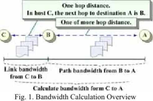
Because only adjacent nodes can hear the reservation information, and the network is multi-hop, the free slots recorded at every node may be different. Here the link bandwidth is defined to be the set of the common free slots between two adjacent nodes. And the path bandwidth between source and destination nodes is the set of available slots on each links along the path. Fig. 1 depicts the bandwidth information/calculation overview.

Fig. 1. Bandwidth Calculation Overview

Fig. 2 illustrates an example for calculating the path bandwidth in more details. The number of data slots in the data frame is 10, and “–” means a reserved slot by the other connections. From this example, path_BW (0,1) = link_BW (0,1) = free_slot(0) ∩ free_slot(1) = {0,7,8}. path_BW(0,2) is calculated from path_BW(0,1) and link_BW(1,2), which is equal to {1,8}. Then

path_BW(0,9) is recursively calculated from path_BW(0,8) and link_BW(8,9) which is equal to

{2,5}. As a result, maximum available bandwidth is two data slots per frame for each link along the entire path. After calculating the end-to-end bandwidth, the data slots need to be reserved from the destination (Node 9) hop-by-hop backward to the source (Node 0). And the reservation wouldn’t be released until the end of the session. In the end, Node 0 begins transmitting datagram on completing the reservation.

Fig. 2. Path Bandwidth Calculation Example

In general, to compute the available bandwidth for a path in a time-slotted network, one not only needs to know the available bandwidth on the links along the path, but also has to determine the scheduling of the free slots. To resolve slot scheduling at the same time as available bandwidth is searched on the entire path is equivalent to solving the SAT problem, which is known to be NP-complete [13].

In this paper, we utilize load statistics to estimate current network remaining bandwidth. Previous papers regarding bandwidth routing focused on TDMA to do bandwidth reservation. It is very complicated both in bandwidth calculation and in reservation. Our solution can estimate bandwidth easily and quickly not only in TDMA networks, but also in IEEE 802.11 networks. We propose a method of bandwidth calculation that is robust to node mobility and traffic dynamics with sacrifice of little statistical errors.

II. THE PROPOSED CALL ADMISSION CONTROL SCHEME

AND BANDWIDTH CALCULATION

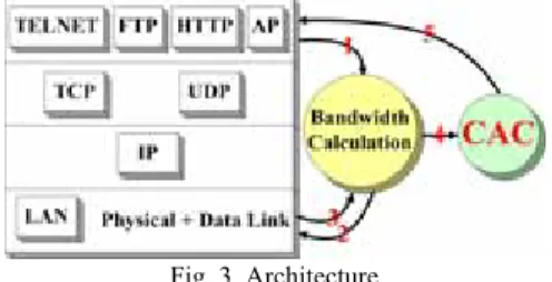
Because the wireless medium resource is scarce, so we want to calculate the present bandwidth and know about if there is enough bandwidth to allow a new flow to achieve the QoS guarantee. So bandwidth calculation is the most important part we want to stress in this paper. According to the information about the bandwidth, we can implement the call admission control scheme. Our objective is to investigate QoS in wireless multi-hop environment. The infrastructure is in Fig. 3 as follows. We plan to add a CAC (Call Admission Control) control procedure into the framework above TCP/UDP layer. Before admitting a new flow entering the network, we have to check if the remaining bandwidth along the path is enough to handle the new request. So when a new application (AP) requests to enter the network (Procedure 1 in Fig. 3), we have to do “bandwidth calculation” first. We

(18)

inquire physical layer about the current channel usage statistics (Procedure 2), and employ the bandwidth calculation method that we proposed to calculate the current bandwidth usage “percentage” (Procedure 3). Then we pass the result to CAC (Procedure 4) to decide if we are going to accept or reject the new flow (Procedure 5).

Fig. 3. Architecture

In bandwidth calculation, we don’t require detailed information such as every slot idle condition. For simplicity, we still think there are slots on a frame basis, although our calculation doesn’t assume TDMA system. We need only information of the average idle percentage during the frame. Assuming that the average idle percentage is equal to the idle percentage for each slot. After getting the idle percentage from each neighbor, we can calculate the common idle percentage of the links, that is, the bandwidth condition we want to know about. With our scheme, even though that there are a large number of slots in a frame, the additional bits (overhead) for transmitting information about the channel condition is fixed. Below, we will discuss the different situations of bandwidth calculation scheme, namely, single-hop, two-hop and multi-hop respectively.

A. Single Hop Path Bandwidth Calculation

A slot is indicated to be busy if the mobile node is transmitting or receiving packets on that slot. In the case of one-hop path, the common idle slots of two adjacent nodes are the slots when they can transmit and receive packets each other. This means the percentage of the common idle slots equal the path bandwidth.

In Fig. 4 as shown, suppose that every slot is independent, x and y indicates the idle percentage (probability) of Node1, and Node2, respectively. n is the (virtual) number of time slots in a frame.

Fig. 4. Single-Hop Induction

Then the common idle probability for each slot is

p=xy, and busy probability is q=1-p. Of n slots, the

probability for having i common idle slots is binomial distribution as follows: n i q p C p n i b n i n i i , 0,1,2,..., ) , ; ( = − = (1)

It is known that mean of the distribution is µ=np, and variance is σ2_{=npq. In other words, of n slots, the}

mean number of common idle slots are nxy, and variance is nxy(1-xy). That is, mean common idle percentage is

n

nxy_{, which equals to xy.}

Fig. 5. Case Description of Single Hop

In more details, we need to know how accuracy of the above estimation for different scenarios. We use Fig. 5 to illustrate the available bandwidth analysis. In the figure, node pairs (i), (ii), and (iii) are interferers. O1 and O2 and observers that represent the one-hop

source/destination pair we want to estimate the path bandwidth. First, if interfering pairs (i), (ii), and (iii) all exists, i.e. hidden terminal problem exists, then the idle percentage is approximately xy (worse case). Secondly, if the two observers sense all the same interfering pairs, for example, only (i) exists in this topology, then the idle percentage is approximately

min(x,y) (best case). Third, if either (i)(ii) or (i)(iii)

exist, then the idle percentage is approximately between xy and min(x,y) (in-between case).

We can also conclude min(x,y) and xy as the upper and lower bounds of one-hop path bandwidth estimation, respectively. It will depend on whether routing protocols can provide the information to choose the appropriate calculation. If there is no information about the topology, then we just choose the lower bound, namely xy.

B. Two Hop Path Bandwidth Calculation

Similarly, assume in Fig. 6 x, y, and z indicates channel idle probability of Node1, Node2 and Node3 respectively. The key point is that the relaying node (Node 2 in the Fig. 6) can’t transmit and receive data at the same slots.

(19)

Fig. 6. Induction of Two-Hop

Assume A (B) is the mean common idle percentage between Node 1 & 2 (2 & 3). Assume C is the mean common idle percentage among all nodes (1, 2, 3). Then we have A=xy, B=yz, C=xyz. Then we can use (A-C) + half of C percentage of bandwidth to transmit data between Node 1 & 2, and use (B-C) + half of C percentage to transmit data between Node 2 & 3. Therefore, the mean idle percentage of the 2-hop path

bandwidth (Node1-Node2-Node3) is _min[ ₍₁ _), ₍₁ _)]

2 xy z yz x

xyz ₊ ₋ ₋ _.

Variance A=xy(1-xy), B=zy(1-yz), C=xyz(1-xyz). The variance of idle percentage of the path Node1-Node2-Node3 is )] 1 )( 1 ( ), 1 )( 1 ( min[ 2 ) 1 ( xyz yz x yz xyz xy z xy xyz xyz − ₊ ₋ ₋ ₋ ₋ ₋ ₋

Similar to single-hop, the two-hop available bandwidth analysis is as follows. If the transmitting pairs around the observers are not all the same to them, then the idle percentage of this two-hop link is _min[ ₍₁ _), ₍₁ _)]

2 xy z yz x

xyz ₊ ₋ ₋ _{(lower bound).}

If Node 1 and Node 2 sense the same traffic flows around them, or Node 2 and Node 3 sense the same traffic flows, then the idle percentage of the link is

min(x,y,z) (upper bound). And we also have the

in-between case here.

C. Multi Hop Path Bandwidth Calculation

In the multi-hop case, the proposed solution is to extend the solution of the above two-hop bandwidth calculation. As in Fig. 7, i, j, k indicate the idle percentage of A to C, B to D, C to E (all two-hop distance) respectively. And the idle percentage of the whole path from A to E is min(i,j,k).

Fig. 7. Induction of Multi-Hop

D. Bandwidth Routing and Call Admission Control Policy

There are many routing protocols for ad hoc mobile wireless networks. Here we choose DSDV as our starting point since it is simple. We extend the DSDV routing protocol to further include the bandwidth information in the routing table.

Our call admission control policy does not need to reserve any bandwidth at call set up time. When a new flow requests to enter the network, it is admitted if the path bandwidth calculation has enough available bandwidth for the request. We are assuming that the path bandwidth calculation is performed every time the routing information exchange. The call admission control policy is performed only at the source node.

III. SIMULATION RESULTS

We use the SimReal Inc. NCTUns 1.0 network simulator [8] and simulate on IEEE 802.11b wireless unslotted system. We also take in account different interfering pairs to simulate several kinds of situation in single-hop, two-hop and multi-hop cases to evaluate our proposed bandwidth calculation scheme. We compare the error percentage between the estimated (our proposed formula) and real (according to log files) bandwidth percentage to see if the error percentage is acceptable. The below figures are the topologies we simulate, Node O1 (or O2, O3) are the observers which

sense the channel activity (busy or idle). Interfering pairs, Node IS transmits data flow to ID through

UDP/CBR/VBR.

A. Single Hop Path Bandwidth Evaluation

Fig. 8 are several single-hop network topologies we simulate to evaluate our proposed bandwidth estimation. We change different external traffic load (IS to ID) during the simulation. Node O1 and O2 are

the observers, and don’t have data flow between them at this time being.

Case 1-1 is the simplest case that O1 and O2 only

observe one transmitting pair (IS to ID). O1 and O2 are

both in the transmission ranges of IS and ID. We

change different loading through IS to ID. Both CBR

and VBR traffic, we use the bandwidth information observed from O1 and O2 to calculate the bandwidth

utilization percentage between them. We also calculate the real idle percentage from the log file, and compare with the estimated value.

(20)

1-1 _1-2

1-3 1-4

1-5

Fig. 8. Single Hop Topologies

Fig. 9 shows the comparison of the link O1-O2

bandwidth between estimated idle percentage and the real idle percentage in the single-hop case 1-1.

Fig. 9. Case 1-1 in Single Hop Topology

In Fig. 8 case 1-2, there are two interfering pairs, and O1 and O2 are in the ranges of two external traffic

flows. There is no hidden terminal to either observer in this case. O1 and O2 both observe the same traffic

flows, so our estimated idle percentage here is the minimal value of O1 and O2 idle percentage. The

following Fig. 10 is the comparison result.

Next, we see 1-3, which has two interferers but they are totally independent to the two observers O1 and O2.

That is, O1 is only affected by IS1 to ID1, and O2 is only

influenced by IS2 to ID2. IS1 and ID1 are the hidden

terminals to O2. The idle percentage between O1 and

O2 is xy (explained before), and Fig. 11 is the result.

Case 1-4 is a little more complicated than 1-3. We add another interfering pair (IS3 to ID3). That means,

each O1 and O2 has one independent interfering pair,

and they also observe the same traffic flow IS3 to ID3.

In this case, the idle percentage of link O1 to O2 is the

lower bound xy.

Mostly, the result of VBR traffic flows has the better accuracy than CBR traffic, and we can see that CBR

(21)

curve in Fig. 12 is a little more irregular.

Case 1-5 is the last case we simulate in single-hop topologies. In the case, O1 is affected by two external

traffic flows IS1 to ID1 and IS2 to ID2, but O2 is only

terminals to O2. So we derive from the previous

inference that the idle percentage in this case is xy. Fig. 13 is the simulation result.

B. Two Hop Path Bandwidth Evaluation

2-1

2-2 2-3

Fig. 14. Two-Hop Topologies

Fig. 14 are the two-hop network topologies we simulate to evaluate our bandwidth calculation scheme. Here we still change different external traffic load (IS

to ID) in each topology. O1, O2 and O3 are the

observers, and don’t’ have data flow between them at this time being. O1 to O3 are two hop distances, and we

use these three different scenarios to compare the accuracy.

Case 2-1 is the simplest case that O1, O2 and O3 all

observe the same transmitting pair (IS to ID). O1, O2

and O3 are all in the transmission ranges of IS and ID,

and the link O1 to O3 is two-hop distances. We change

different loading through IS to ID. For both CBR and

VBR traffic, we use the bandwidth information observed from O1, O2 and O3 to calculate the

bandwidth utilization percentage between them. We also calculate the real idle percentage from the log file, and compare with the estimated value.

Fig. 15 shows the comparison of the O1 to O3 path

bandwidth between estimated idle percentage and the real idle percentage in the two-hop case 2-1.

Fig. 15. Case 2-1 in Two Hop Topology

Next, in Case 2-2, there are two interfering pairs that are totally independent to the two observers O1 and O3.

That is, O1 is only affected by IS1 to ID1, and O3 is only

terminals to O2. O3 here is out of the range of the two

external traffic flows. The idle percentage between O1

and O3 is the lower bound case, and Fig. 16 is the

result.

Case 2-3 is more complicated than 2-2. We add another interfering pair (IS3 to ID3). That means, O1

and O3 has one independent interfering pair, and also

observe the same traffic flow IS3 to ID3. The idle

percentage of link O1 to O3 here is using the lower

bound.

(22)

see that the result of 2-3 has larger error percentage than all the other scenarios. It might be due that this case is in-between case, while we use lower bound to calculate.

C. Multi Hop Path Bandwidth Evaluation

3-1 3-2

Fig. 18. Multi-Hop Topologies

Fig. 18 are the multi-hop network topologies we simulate to evaluate our bandwidth calculation scheme. Here we still change different external traffic load (IS

to ID) in each topology. O1, O2, O3 and O4 are the

observers again don’t have data flow between them at the time being. O1 to O3 and O2 to O4 are two hop

distances, and we use these two different scenarios to observe the accuracy of the estimation in multi-hop cases.

Fig. 19. Case 3-1 in Multi Hop Topology

In Case 3-1, O1 is only in the transmission range of

IS1 and ID1. O2 and O3 are out of the transmission

ranges of all the interferers, and O4 is in the

transmission range of IS2 and ID2. We change different

loading through IS1 to ID1 and IS2 to ID2 with both CBR

and VBR traffic. Then we use the bandwidth information observed from O1, O2, O3 and O4 to

calculate the bandwidth utilization percentage between them. We also calculate the real idle percentage from the log file, and compare with the estimated value. Fig. 19 shows the comparison of the O1 to O4 link between

estimated idle percentage and the real idle percentage in the multi-hop cases.

Fig. 20. Case 3-2 in Multi Hop Topology

In Case 3-2, O1 is only in the transmission range of

IS1 and ID1. O2 is out of the transmission ranges of all

the interferers. O3 is in the transmission range of both

IS2 to ID2 and IS3 to ID3, and O4 is only in the

transmission range of IS3 and ID3. Again, we change

different loading through IS1 to ID1, IS2 to ID2, and IS3 to

ID3. For both CBR and VBR traffic, we use the

bandwidth information observed from O1, O2, O3 and

O4 to calculate the bandwidth utilization percentage of

whole path from O1 to O4 through this topology. We

also calculate the real idle percentage from the log file, and compare with the estimated value. Fig. 20 is the result.

(23)

Moreover, we also try to put real traffic in the observer pairs to verify if the bandwidth estimation is correct enough. Here we add additionally different CBR and VBR traffic loading in the original 1-1 scenario. We compare the maximal available remaining bandwidth between the estimation and real network traffic through the throughput information we obtained. Fig. 21 indicates the available bandwidth comparison of both CBR and VBR traffic cases.

Similarly, we also experiment different CBR and VBR traffic load (O1 to O3) in the original 2-1 scenario.

Then we can compare the maximal available remaining bandwidth between the estimation and real network traffic through the throughput information we obtained. Fig. 22 depicts the comparison of CBR and VBR traffic.

Same thing here, we also add different CBR and VBR traffic load (O1 to O4) in the original 3-1 scenario.

Then we can compare the maximal available remaining bandwidth between the estimation and real network traffic through the throughput information we obtained. Fig. 23 depicts the comparison of CBR and VBR traffic.

D. Integrated Scenario

Finally, we evaluate our bandwidth calculation in a more typical wireless multi-hop topology as shown in

Fig. 24. Here we fix three interfering pairs {F,G}, {C,D}, and {E,K} as background traffic and vary the total traffic loads. Then we choose several S/D (Source/Destination) pairs randomly which might be single-hop, two-hop or multi-hop in different time scales. We evaluate their efficiency for supporting QoS. We define ATR (Achieved Throughput Ratio) for S/D pairs as one of the efficiency metrics.

) ( EstimatedBandwidth d OfferedLoa Throughput ATR = = (2)

100% of ATR is the perfect situation, which means that we could efficiently use the available bandwidth as we estimated. Normalized one-hop average delay represents another efficiency metrics. Because S/D pair is randomly chosen, so we normalize the delay time to one-hop distance delay time and get the average.

Fig. 24. Integrated Scenario

Fig. 25 is the simulation result that depicts the average achieved throughput ratio. The ATR decreases slightly while the background traffic loading increases. Overall, the average ATR are acceptable which are almost above 85%. Although there exists statistical inaccuracy in our solution, our proposed estimate still get stable results even we ignore the IEEE 802.11 MAC overhead.

Fig. 25. Average Achieved Throughput Ratio

Fig. 26 shows the normalized delay time of the simulation. The mean normalized delay time jumps with the increase of traffic load. The VBR traffic delay time ascends more obviously than CBR traffic

全域性無線數位家庭多媒體網路管理

行政院國家科學委員會專題研究計畫 成果報告