決策球模式之建構與應用

國

立

交

通

大

學

資訊管理研究所

博

士

論

文

決策球模式之建構與應用

Decision Ball Models: Methods and Applications

研 究 生：馬麗菁

指導教授：黎漢林 教授

決策球模式之建構與應用

Decision Ball Models: Methods and Applications

研 究 生：馬麗菁 Student：Li-Ching Ma

指導教授：黎漢林 Advisor：Han-Lin Li

國 立 交 通 大 學

資 訊 管 理 研 究 所

博 士 論 文

Submitted to Institute of Information Management College of Management

National Chiao Tung University in partial Fulfillment of the Requirements

for the Degree of Doctor of Philosophy

in

Information Management

June 2006

Hsinchu, Taiwan, Republic of China

決策球模式之建構與應用

學生：馬麗菁 指導教授

黎漢林

國立交通大學資訊管理研究所博士班

摘 要

Decision Ball Models: Methods and Applications

Student：Li-Ching Ma Advisor: Han-Lin Li

Institute of Information Management National Chiao Tung University

ABSTRACT

Decision makers’ preferences are often influenced by background information. This

study develops a Decision Ball system to provide visual context and similarity analysis to

help decision makers to reach a better decision. The proposed Decision Ball system includes

four types of Decision Ball models: Franklin’s Moral Algebra models, Even Swap models,

Pairwise Comparison models, and Classification models. Franklin’s Moral Algebra Decision

Ball models solve “Yes” or “No” decision problem. Even Swap and Pairwise Comparison

Decision Ball models are for ranking problems with multiple alternatives. Classification

Decision Ball models treat group problem. The proposed approach can be applied in a variety

of decision problems. For instance, a Decision Ball system can assist decision makers in

personal decision-making problem, operational and managerial decision problems, and

financial decision problems, etc.

誌 謝

終於，我做到了! 博士論文的完成，首先要感謝的是指導教授黎漢林老

師，他除了教導我專業知識外，更讓我學習到如何成為一位受人尊敬的老

師與學者。同時，也要感謝論文口試委員溫于平教授、蘇朝墩教授、陳安

斌教授及林妙聰教授於口試時提供了許多寶貴的意見與建議，使本論文更

趨完善。

在研究室共同奮鬥的日子是令人懷念的，芸珊、昶瑞、明賢、宇謙、志

信、嘉輝、治華、俊慶和玉雯，有幸和你們共渡這段特別的時光，有你們

相伴，讓我在交大的日子總是充實且快樂的。感謝榮發及曜輝，在系統開

發上的協助與支援。此外，也要感謝國立聯合大學同事們的支持與勉勵。

求學期間，感謝公公、婆婆的協助, 讓我無後顧之憂。感謝父母親的教

誨與鼓勵，雖然敬愛的母親已於我博二時往生，她的關愛永遠伴隨著我。

最後，感謝我親愛的老公，一路陪伴著我，分擔我的情緒與壓力，在我脆

弱的時候，給我依靠與鼓勵，讓我有足夠的勇氣繼續往前。也謝謝兩個淘

氣可愛的兒子，沒為我找太多的麻煩，讓我能安心求學，家人的支持是我

最大的力量。

Contents

1.1 Research Motivation and Purposes……….. 1

1.2 Advantages of Decision Balls……….. 3

1.3 Framework of the Proposed Decision Ball System……….. 5

1.4 Structure of the Dissertation………10

Chapter 2 Review of Visualization Tools………..12

2.1 Review of Multidimensional Scaling (MDS) Techniques……….. 12

2.2 Review of Gower Plots……….. 15

2.3 Summary……….19

3.1 Properties of Additive Score Functions……….. 20

3.2 Properties of Multiplicative Score Functions………. 22

3.3 Display Techniques………. 24

3.4 An Illustrative Example – Visualization on Decision Balls………25

3.5 Summary………. 28

Chapter 4 Model 1: Moral Algebra Decision Ball Models……….. 29

4.1 Introduction to Franklin’s Moral Algebra………... 29

4.2 Construction of Moral Algebra Decision Ball Models………32

4.3 An Illustrative example – A CEO’s dilemma………. 34

4.4 Summary………..43

Chapter 5 Model 2: Even Swap Decision Ball Models……….45

5.1 Introduction to Even Swaps……… 45

5.2 Construction of Even Swap Decision Ball Models……… 48

5.3 An Illustrative Example – An Office-Renting Problem…………. 54

5.4 Summary……… 61

Chapter 6 Model 3: Pairwise Comparison Decision Ball Models……… 62

6.1 Introduction to Pairwise Comparisons……… 63

6.2 Construction of Pairwise Comparison Decision Ball Models…… 67

Selection of Universities………. 72

6.4 Summary………. 78

Chapter 7 Model 4: Classification Decision Ball Models……… 81

7.1 Introduction to DEA-DA Analysis………. 81

7.2 Constructions of Classification Decision Ball Models………….. 86

7.3 Illustrative Examples – A Corporate Bankruptcy Example……… 91

and Japanese Banks 7.4 Summary……… 101

Chapter 8 Concluding Remarks……… 103

References……… 105

Tables

Table 3.1 Data matrix of Example 3.1……… 26

Table 3.2 Results of Example 3.1 with an additive score function ……… 26

Table 3.3 Results of Example 3.1 with a multiplicative score function………..27

Table 4.1 The relationship between two options……….32

Table 4.2 The mapping table of relationship type and distance………..33

Table 4.3 David’s list of pros and cons for accepting the new position……….. 37

Table 5.1 The consequence table of Example 1……….. 55

Table 6.1 Improvements in inconsistency measured by consistency ratio (CR)…….80

Table 7.1 Financial performance of 83 firms in US electric power industry……….. 92

Figures

Figure 1.1 Visual background in decision environment……….. 2

Figure 1.2 Advantages of Decision Balls………. 4

Figure 1.3 Framework of the proposed Decision Ball System………. 6

Figure 1.4 Structure of the dissertation……….. 11

Figure 2.1 Displaying a distance matrix R1 by non-metric MDS techniques……….15

Figure 2.2 Gower Plots of R2………..18

Figure 3.1 The Decision Ball of Example 3.1 with an additive score function……..27

Figure 3.2 The Decision Ball of Example 3.1 with a multiplicative score function.. 28

Figure 4.1 Pro Ball of Example 4.1……… 38

Figure 4.2 Con Ball of Example 4.1………... 39

Figure 4.3 Pro-Con Ball of Example 4.1……….42

Figure 5.1 Moving trajectory of concurrent points………. 52

Figure 5.2 The decision ball and even swaps after Iteration 1……… 59

Figure 5.3 The decision ball and even swaps after Iteration 2………59

Figure 5.4 The decision ball and even swaps after Iteration 3……… 59

Figure 5.5 The decision ball and even swaps after Iteration 4………60

Figure 5.7 The moving trajectories of A3 and A4 after even swaps………. 60

Figure 6.1 Solution procedure of Pairwise Comparison Decision Ball models……..66

Figure 6.2 Decision Process of Example 6.1……….. 75

Figure 6.3 Decision Process of Example 6.2……….. 78

Figure 7.1 The visual structure of the standard MIP approach………85

Figure 7.2 The visual structure of the two-stage MIP approach………..85

Figure 7.3 The conceptual diagram of the multi-layer Classification Decision Ball models……… 88

Figure 7.4 The multi-stage classifying processes of the proposed Classification Decision Ball models………. 90

Figure 7.5 The Decision Ball of 10 target observations………..94

Figure 7.6 The Decision Ball of observation 62 based on the target observations… 95 Figure 7.7 The first layer Decision Ball of Example 7.2……… 98

Figure 7.8 The second layer Decision Ball of Example 7.2……… 100

Chapter 1 Introduction

Ranking and grouping alternatives are two of major challenges in decision-making. The

more decision alternatives and criteria are being considered, the more difficulties the decision

maker (DM) has to face. Therefore, how to assist the decision maker make a more reliable

and knowledgeable decision is a very important issue.

1.1 Research Motivation and Purposes

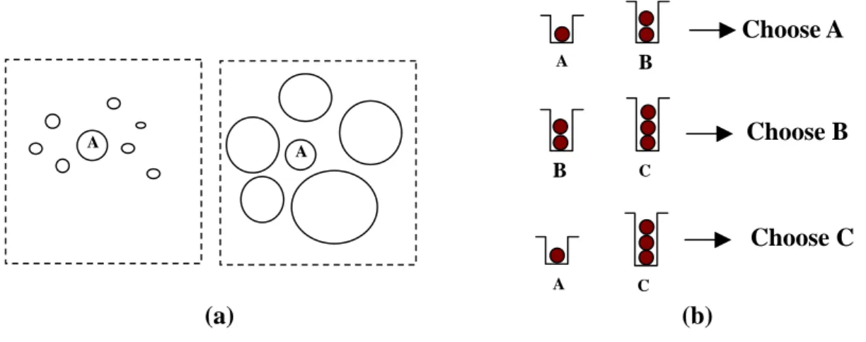
Consumer choice theories show that consumer choice is often affected by context

(Seiford and Zhu, 2003). For instance, a circle appears large when surrounded by small circles

and small when surrounded by larger ones, as shown in Figure 1.1(a). Similarly, a product

may appear attractive against a background of less attractive alternatives and unattractive

when compared to more attractive alternatives (Simonson and Tversky, 1992). Tversky and

Simonson (1993) showed the relative attractiveness of x compared to y often depends on the

presence or absence of a third option z. In addition, Keeney (2002) identified 12 important

mistakes frequently made that limit one’s ability to determine useful value trade-offs, in

which “not understanding the Decision Context” is the first critical mistake.

Even animals’ choice is heavily affected by what visual background they have seen. In

in Figure 1.1(b). There are three options: A, B and C. A is for one raisin in a short tube. B is

for two raisins in a medium length tube, and C is for three raisins in a long tube. When

displaying A and B to a jay, it will choose A. When displaying B and C to a jay, it prefers B.

However, by displaying A and C to a jay, it prefers C. If the choices, A, B and C could be

displayed to the gray jay simultaneously, it might make a better decision. Therefore, how to

assist decision makers visualize the background information is an important issue in

decision-making.

Ranking alternatives is one of the most important challenges in decision-making,

especially when involving inconsistencies. If a decision maker’s judgment is highly

inconsistent, different ranking methods may produce wildly different priorities. That is, the

decision maker may not make a reliable decision. Hence, how to assist the decision makers

detect and improve these inconsistencies is another important issue in decision-making.

This study proposes Decision Ball models to provide visual representation of ranks of

and similarities among alternatives, thus to help the decision makers make a more

Figure 1.1 Visual background in decision environment (a) Influence of visual background (b) Gray jay’s choice

A C A _B B C Choose A Choose B A Choose C A (a) (b)

knowledgeable decision. Four types of Decision Ball models are constructed to meet the

decision makers with different decision preferences and requirements. In addition, this study

tries to help a decision maker improve the quality of his/her decision-making by reducing

serious inconsistencies in judgment.

The major advantages of the proposed approach for a decision maker are summarized as

below:

(i) Make a more knowledgeable decision through visualizing background information and

decision processes.

(ii) Make a more reliable decision by improving inconsistencies iteratively.

(iii) Select a type of Decision Ball models based on his/her decision preferences and

requirements.

(iv) Observe the ranks of and similarities among alternatives on Decision Balls directly.

(v) See the grouping relationships among alternatives layer-by-layer on Decision Balls, and

perceive the benchmark alternatives if the DM would like to upgrade the performance of

an alternative from one group to another.

1.2 Advantages of Decision Balls

Decision Ball models display alternatives on the surface of a ball. The arc length

difference, the longer the arc length. In addition, the alternative with a higher score is

designed to be closer to the North Pole so that alternatives will be located on the concentric

circles in the order of rank from top view.

The advantages of Decision Balls are illustrated as follows:

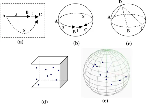
(i) Comparing with 2-Dimensional plane models, Decision Balls can depict three points that

do not obey the triangular inequality (i.e. the total length of any two edges must be larger

than the length of the third edge). For instance, given three options A, B, and C. Suppose

the distance between A and B is 3; the distance between B and C is 1; the distance

between A and C is 6. We cannot draw three lines to connect A, B and C (Figure

Figure 1.2 Advantages of Decision Balls (a) Display line segments on a 2-D plane (b) Display curves on a ball (c) Display four points that are not

on the same plane (d) Display points in a 3-D cube (e) Display points on the surface of a ball

A 3 B 1 C 6 A B C 6 1 3 A B C D (a) _{(b) (c)} (e) (d)

1.2(a)). However, it is convenient to draw three arcs on the surface of a ball to illustrate

their relationships (Figure 1.2(b)).

(ii) Decision Ball models are better than 2-Dimensional plane models because the former

can show four points which are not on the same plane, as shown in Figure 1.2(c).

(iii) Comparing with 3-Dimensional cube models (Figure 1.2(d)), Decision Ball models are

easier for a decision maker to observe the relationship among alternatives than

3-Dimensional cube models because the former can exhibit points on the surface of a

ball, as shown in Figure1.2 (d) and (e).

(iv) Decision Ball models can depict inconsistencies in the decision makers’ judgments.

(Discussed in Chapter 5 and 6).

(v) A Decision Ball can display both ranks of and similarities among alternatives.

(vi) A Decision Ball involves no edges.

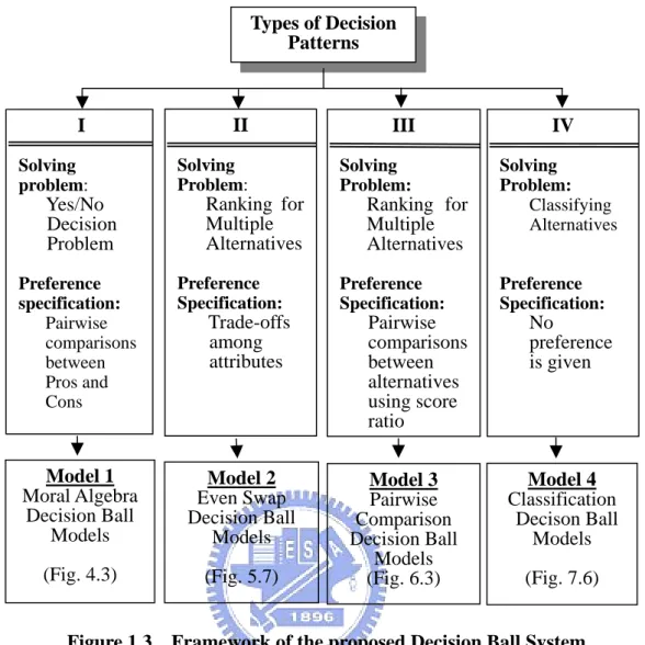
1.3 Framework of the Proposed Decision Ball System

Different decision makers may have various decision preferences and requirements

because of personality of a decision maker, complexity of a decision problem, availability of

decision data, …etc. This study summarizes four popular types of decision patterns and

proposes corresponding Decision Ball models as follows: (Figure 1.3)

Types of Decision Patterns

The decision makers are assumed to make a binary choice, or a “Yes or No” decision

problem. This is the simplest decision pattern because the decision makers have not to

estimate the value of each criterion for each alternative in advance.

Franklin (1956) proposed a process to help a decision maker make a rational choice under

this decision pattern, called Franklin’s Moral or Prudential Algebra. Franklin’s Moral Algebra

for making choices was first to divide a sheet of paper into two columns; one for pro, and

another for con. Then, write down the various motives, for or against the choice. If a reason

pro equaled a reason con, then both would be crossed out. If a reason pro equaled two reasons I Solving problem: Yes/No Decision Problem Preference specification: Pairwise comparisons between Pros and Cons Model 1 Moral Algebra Decision Ball Models (Fig. 4.3) Model 2 Even Swap Decision Ball Models (Fig. 5.7) Model 3 Pairwise Comparison Decision Ball Models (Fig. 6.3) Model 4 Classification Decison Ball Models (Fig. 7.6) II Solving Problem: Ranking for Multiple Alternatives Preference Specification: Trade-offs among attributes III Solving Problem: Ranking for Multiple Alternatives Preference Specification: Pairwise comparisons between alternatives using score ratio IV Solving Problem: Classifying Alternatives Preference Specification: No preference is given

con, the three were crossed out. After a day or two of consideration, if nothing new came to

mind for either side, the decision maker could then come to a determination.

Franklin’s Moral Algebra is an intelligent way of simplifying the complexity of a

decision. However, it is not easy for a decision maker to tell explicitly which pro(s) and con(s)

can be eliminated simultaneously.

This study proposes Moral Algebra Decision Ball models to improve the insufficiencies

of Franklin’s Moral Algebra. Decision makers are assumed to be able to make pairwise

comparisons between pro and con reasons with words such as “equally important”, “slightly

more important”, “more important” and “significantly more important”. By visualizing the

relationships between pros and cons on Decision Balls, the decision makers can make a more

knowledgeable decision.

(ii) Type II Pattern

Ranking for multiple alternatives is the major type of decision problem considered here.

This pattern is sophisticated because the decision makers must be capable of making clear

trade-offs among a range of criteria across a range of alternatives.

Hammond et al. (1998) developed a mechanism of Even Swaps to provide a useful way

of making trade-offs. “Even” implies equivalence and “Swap” represents exchange. An even

swap increases the value of one criterion while decreasing the value by an equivalent amount

number of criteria, the most preferred alternative could be found.

Even swap approach is a rational and practically useful way in finding the best

alternative. However, the ranks of rest of alternatives are not known, and there may exist large

inconsistencies among even swaps that the DM could not know.

This study presents Even Swap Decision Ball models to assist the DM observe the ranks

of and similarities among alternatives on the Decision Ball. The superiority relationship

between alternatives can be observed by checking the longitude of alternatives. The

inconsistencies between even swaps can also be known by checking the latitude of

alternatives.

(iii) Type III Pattern

Ranking for multiple alternatives is the type of decision problem solved in this pattern

too. However, instead of making trade-offs explicitly among values of criteria in Type II

pattern, the decision makers of this decision pattern make pairwise comparisons between

alternatives using score ratios.

The analytic hierarchy process (AHP)(Saaty, 1977, 1980; Saaty and Vargas, 1984, 1994)

has been used widely to determine relative ranking of the decision alternatives through the

pairwise comparison of alternatives at each level of the hierarchy. However, if perturbations

from consistency are large, the information available cannot be used to derive a reliable

priorities if a preference matrix is highly inconsistent. Hence, how to help the decision makers

detect and adjust these inconsistencies becomes an important issue in this decision pattern.

This study illustrates Pairwise Comparison Decision Ball models to help the DM make a

more reliable decision by detecting and improving inconsistencies in judgments. In addition

to the ranks of and similarities among alternatives, the DM can observe the suggestions for

effectively reducing inconsistencies on Decision Balls.

(iv) Type IV pattern

In this decision pattern, the decision makers do not have personal preferences about

alternatives. They are interested in classifying alternatives more than ranking alternatives.

Discriminant Analysis (DA) is a statistical technique and popular method for predicting

group membership. The GP (Goal Programming)-based DA, first proposed by Freed and

Glover (1981), can estimate weights of criteria by minimizing sum of deviations (MSD, Freed

and Glover, 1986) or minimizing misclassified alternatives (MMO, Banks and Abad, 1991).

Those weights yield an evaluation score, which is compared with a threshold value for

classifying alternatives. Sueyoshi (1999) first proposed a DEA-DA analysis incorporating the

non-parametric feature of Data Envelopment Analysis (DEA, Charnes et al., 1978) into the

DA. DEA-DA approach can effectively improve hit rates. However, it includes too many

binary variables, and the decision makers cannot “see” the grouping relationships via

This study presents Classification Decision Ball models to aid the decision makers

observe the grouping relationships on Decision Balls layer by layer. In addition to the ranks of

and similarities among alternatives, the DMs can perceive the benchmark alternatives if the

DMs would like to upgrade the performance of an alternative from one group to another. The

number of binary variables can also be reduced significantly.

The framework of the proposed Decision Ball system is shown in Figure 1.3. Each type

of decision patterns is illustrated as solving problem and preference specification parts. The

corresponding Decision Ball models are depicted in the lower part of Figure 1.3.

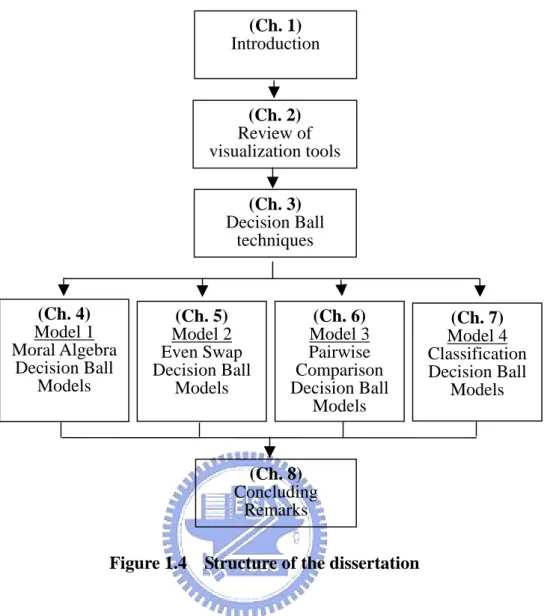
1.4 Structure of the dissertation

The structure of this dissertation is depicted in Figure 1.4 and briefly introduced as

follows:

Chapter 2 reviews two popular visualization tools: Multidimensional Scaling (Cox and

Cox, 2000) and Gower Plots (Gower, 1977; Genest and Zhang, 1996). Their advantages and

insufficiencies are also discussed.

Chapter 3 introduces Decision Ball techniques. The properties of additive score

functions and multiplicative score functions are discussed first. Then, the Decision Ball

techniques, based on the concept of Multidimensional Scaling, are presented. How to display

Chapter 4 presents Model 1 – Moral Algebra Decision Ball models for Type I decision

pattern. The process of Franklin’s Moral Algebra is described first. Moral Algebra Decision

Ball models are then constructed. An example of a CEO’s dilemma is illustrated to

demonstrate the decision processes.

Chapter 5 discusses Model 2 – Even Swap Decision Ball models for Type II decision

pattern. The method of Even Swaps is introduced. Then corresponding Even Swap Decision

Ball models are built. An office-renting problem is used as an illustrative example. Chapter 6

addresses Model 3 – Pairwise Comparison Decision Ball models for Type III decision pattern.

(Ch. 4) Model 1 Moral Algebra Decision Ball Models (Ch. 5) Model 2 Even Swap Decision Ball Models (Ch. 6) Model 3 Pairwise Comparison Decision Ball Models (Ch. 1) Introduction (Ch. 2) Review of visualization tools (Ch. 8) Concluding Remarks (Ch. 3) Decision Ball techniques

Figure 1.4 Structure of the dissertation

(Ch. 7)

Model 4 Classification Decision Ball

This chapter first describes the basic concept of pairwise comparison, and then creates

Pairwise Comparison Decision Ball models. Gower Plots are adopted to detect alternatives

causing major inconsistencies. Optimization models are proposed to help the DM improve

these inconsistencies conveniently. Two examples, investment in mutual funds and selection

of universities, are demonstrated in this chapter.

Chapter 7 presents Model 4 – Classification Decision Ball models for Type IV decision

pattern. DEA-DA analysis is introduced, and the Classification Decision Ball models are

formed. Then, a corporate bankruptcy example and an example of Japanese banks are

demonstrated. Chapter 8 presents concluding remarks and suggests directions for future

Chapter 2 Review of Visualization Tools

Several graphical techniques have been developed to aid the DM visualize background

information. For instance, Li (1999) used deduction graphs to treat decision problems

associated with expanding competence sets. Gower (1977), Genest and Zhang (1996)

proposed a powerful graphical tool, the so-called Gower Plot, to detect the cardinal and

ordinal inconsistencies in decision maker’s preferences. Multidimensional Scaling (Borg and

Groenen, 1997; Cox and Cox, 2000) is a classical technique used to provide a visual

representation of similarities among a set of alternatives.

This chapter briefly reviews two popular visualization techniques, Multidimensional

Scaling techniques and Gower Plots, which are adopted and compared in this study.

The structure of this chapter is organized as follows. Section 2.1 illustrates the

Multidimensional Scaling technique. Section 2.2 briefly reviews Gower Plots method.

Summary of this chapter is made in Section 2.3.

2.1 Review of Multidimensional Scaling (MDS) Techniques

Multidimensional Scaling (Borg and Groenen, 1997; Cox and Cox, 2000) is a classical

technique to provide a visual representation of similarities among a set of alternatives, which

dimensional space (usually Euclidean).

There are two major forms of MDS: metric and non-metric MDS. In metric scaling, the

dissimilarities between all objects are known numbers, which can be approximated by

distances directly. In non-metric MDS, only the rank order of the dissimilarities is

approximated: the larger the dissimilarity, the longer the distance. Several MDS models (Cox

and Cox, 2000) have been developed. One of commonly used model is proposed by Kruskal

(1964a, 1964b). He developed a numerical measure of the closeness between the

dissimilarities in the lower dimensional and the original spaces, called Stress. Denote di,j as

distance and δi,j as dissimilarity between alternative Ai and Aj. Stress can be formulated as

∑∑

∑∑

where f(δi, j) is the transformation of the δi, j . In metric scaling, f(δi, j) is a linear

transformation of δi, j . In non-metric scaling, f(δi, j) is a weakly monotonic

transformation of δi, j . That is, if δi, j < δp,q , )f(δi,j)≤ f(δp,q . The Stress has a value

between 0 and 1, with 0 indicating perfect fit and 1 implying worst possible fit. The rule of

thumb for the value of Stress is that anything under 0.1 is excellent and over 0.15 is

unacceptable. Based on Kruskal’s approach, an initial configuration is randomly specified.

Then an iterative procedure based on the steepest descent method is applied to move toward a

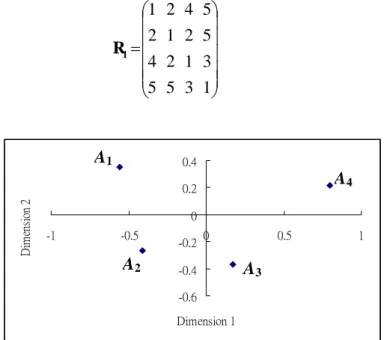
⎟⎟ ⎟ ⎟ ⎟ ⎠ ⎞ ⎜⎜ ⎜ ⎜ ⎜ ⎝ ⎛ = 1 3 5 5 3 1 2 4 5 2 1 2 5 4 2 1 1 R -0.6 -0.4 -0.2 0 0.2 0.4 -1 -0.5 0 0.5 1 Dimension 1 D im en si on 2 A1 A A2 _A3 4

Figure 2.1 Displaying a distance matrix R1 by non-metric MDS

techniques

For instance, a distance matrix R1, with four alternative A1, A2, A3, and A4, can be

visualized by non-metric MDS techniques as shown in Figure 2.1. The Stress of this visual

presentation is 0.57%.

Conventional MDS models, including Kruskal’s approach, can effectively provide a

visual representation of dissimilarities among objects. However, the conventional

multidimensional scaling technique cannot show the ranks of alternatives and is incapable of

detecting and adjusting inconsistencies in the decision makers’ preferences.

2.2 Review of Gower Plots

Genest and Zhang (1996) proposed a graphical method, which is close in spirit to MDS,

work of Gower (Gower, 1977), can display both the inconsistencies of data matrix and the

ranks of alternatives. This section briefly introduces the mathematical properties of Gower

Plots. The detail explanations of Gower Plots can refer to Genest and Zhang (1996).

The singular values of a matrix M of rank n are the positive square roots of the

eigenvalues of the symmetric matrix MTM, where MTstands for transposition of M. If M is skew-symmetric, i.e. MT = -M, the singular values of the matrix M are equal to the norm of its purely imaginary eigenvalues.

Let 0λ1 ≥K≥λm ≥ (and λm+1 =0 if n is an odd number) represent those singular

values, with m indicating the integer part of n/2. Using singular value decomposition (Horn

and Johnson, 1985), a skew-symmetric matrix M can be decomposed into the form

) ( 2 1 2 2 2 1 1 T j j T j j m j j − − = − =

∑

where U2j-1and U2j are orthonormal eigenvectors of MTM corresponding to λ2j.

The matrix M* = (λ1 UVT −VUT) with U = U1 and V= U2 provides the best approximation of a skew-symmetric matrix M of rank two, because the first term of M gives

the best least-squares fit of rank two to M (Eckart and Young, 1936). Let U = (u1, …, un)T

and V = (v1, …, vn)T as n points Pj = (uj, vj) in the plane. A Gower Plot of a skew-symmetric

matrix M is a two-dimensional graph composed of all Pj, 1≤ j≤n, on the graph.

variability

∑

Consider a set of n alternatives A1, A2, …, An. Denote ri,j as the ratio of the weights of Ai

to that of Aj, specified as,

j i j i j i e w w r_, = _, , (2.4)

where wi is the weight of Ai, wi > 0, for all . is a multiplicative term accounting for

inconsistencies. It is assumed that r

i ei,j i,j = i j r _, 1

, as illustrated in AHP (Saaty, 1977). Let R =

(ri,j), for all i, , be a j preference matrix. Following Genest and Zhang (1996), a

tournament matrix T = (t n n×

i,j) corresponding to R, is defined as ti,j = 1 if ri,j > 1; ti,j = 0 if ri,j = 1;

ti,j = −1 if ri,j < 1.

Since T is a skew-symmetric matrix, a Gower Plot based on T can be depicted, called

the ordinal Gower Plot of R. From the work of Genest and Zhang (1996), we summarize the

following rules to detect the ordinal consistency of R. Examining the ordinal Gower Plot of

R, R is close to be ordinal consistent, if (i) the location of alternatives (points P1, …, Pn )

are equidistant from origin within a 180 degree arc; (ii) the angles between consecutive points

are equal to 180/n degrees; (iii) the faithfulness of the graphical representation is

demonstrated by variability factor, expressed in (2.3), being approximately 1. The points are

arranged counter-clock-wise in the order of preference.

Plot based on S can be depicted, called the cardinal Gower Plot of R. Examining the cardinal

Gower Plot of R, R is close to be cardinal consistent, if (i) P1, …, Pn are collinear, and (ii)

variability factor is approximately 1. The first condition means that *, , for all

* , * ,k k j i j i s s s + = n j k i ≤ ≤ , , 1 .

For instance, suppose a DM specifies a preference matrix as R2. T2 is the tournament

matrix corresponding to R2. The ordinal Gower Plot is depicted in Figure 2.2(a).

Examining the ordinal Gower Plot, the matrix R2is ordinal consistent because (i) all its points

are located on a half-circle; (ii) the angles between every two consecutive points are equal to

180/n degrees; (iii) variability factor = 97.1%. Let S2 = ln(R2), the cardinal Gower Plot of

R2 is depicted in Fig. 2.2(b) representing 99.9% variability. The matrix R2 is not cardinal

consistent because A4 is away from the collinear line. The ranking of alternatives is A1 f A2

⎟⎟ ⎟ ⎟ ⎟ ⎠ ⎞ ⎜⎜ ⎜ ⎜ ⎜ ⎝ ⎛ = 1 3 / 1 5 / 1 5 / 1 3 1 2 / 1 4 / 1 5 2 1 2 / 1 5 4 2 1 2 R ⎟⎟ ⎟ ⎟ ⎟ ⎠ ⎞ ⎜⎜ ⎜ ⎜ ⎜ ⎝ ⎛ − − − − − − = 0 1 1 1 1 0 1 1 1 1 0 1 1 1 1 0 2 T

f A3 f A4 (“f” means superior to).

Gower Plots are powerful tools for detecting inconsistencies in data matrix, and can also

display ranks of alternatives. However, it can neither show the similarities among alternatives

nor provide any suggestions about how to adjust inconsistencies. In addition, a Gower Plot

2.3 Summary

A decision maker’s choice is often affected by background information. This chapter

briefly reviews two commonly used visualization techniques, Multidimensional Scaling and

Gower Plots, and illustrates their advantages and insufficiencies.

-0.6 -0.4 -0.2 0 0.2 0.4 0.6 0.8 -0.8 -0.6 -0.4 -0.2 0 A1 -0.6 -0.4 -0.2 0 0.2 0.4 0.6 0.8 -0.8 -0.6 -0.4 -0.2 0 A1 A A₂ 2 A3 A3 A4 A4

Figure 2.2 Gower Plots of R2 (a) ordinal Gower Plot of R2 (b) cardinal

Gower Plot of R2

Chapter 3 Decision Ball Techniques

This chapter illustrates the Decision Ball techniques with additive and multiplicative

score functions respectively, based on the concept of Multidimensional Scaling techniques.

An additive score function is the most commonly used form in practice (Belton and

Stewart, 2002) since it is more understandable for the decision maker. However, the linear

additive score function is restricted to a fixed rate of substitution between criteria. A

multiplicative score function is good at reflecting reasonable marginal rate of substitution, but

is more complicated than the additive one. Both score functions are provided here to allow a

decision maker to choose a proper one.

The structure of this chapter is organized as follows. Section 3.1 introduces the

properties of additive score functions. Section 3.2 illustrates the properties of multiplicative

score functions. Section 3.3 proposes the Decision Ball techniques with additive and

multiplicative score functions respectively. Section 3.4 uses an example to demonstrate how

to display alternatives on Decision Balls. Summary of this chapter is made in Section 3.5.

3.1 Properties of Additive Score Functions

Let A = {A1, A2, …, An} be a set of n alternatives for solving a decision problem, where

wk as the weight of criterion k. In order to make sure all weights of criteria are positive, a

criterion ci,k with cost feature (i.e., a DM likes to keep it as small as possible) is transformed

from ci,k to (ck −ci,k) in advance, where ck is the largest value of criterion k.

Notation 3.1 The score function of Ai is assumed in an additive form, expressed below

∑

where (i) wk ≥ 0, ∀k and

∑

= = m k k w 1

1 w=(w1,w2,K,wm) is a weight vector obtained by other decision methods in advance, (ii)ck and ck are respectively the largest and smallest

values of a criterion k. (iii) 0≤Si(w)≤1.

Notation 3.2 The dissimilarity between Ai and Aj is defined as

∑

For the purpose of comparison, we define an ideal alternative A_* , where

) , , , ( _{1 2} * * A c c cm

A = _K and . is designed to be located at the north pole of a ball (radius = 1) with coordinate = (0, 1, 0). Denote

1 * = S A_* ) , , (x* y* z* δi,*, as the dissimilarity, distance between A ,* i d

i and A* respectively. We then have following propositions:

Proposition 3.1 δi,*(w)=1−Si(w) (3.3) <Proof>

∑

∑

) ( 1 ) ) ( ) ( ( 1 1 , w i m k m k _{k k} k k i k k k k k k S c c c c w c c c c w = − − − − − − =

∑

∑

Notation 3.3 Denote the Euclidean distance between Ai and Aj as

di,j = 2δi,j, (3.4)

such that if δi,j = 0 then di,j = 0 and if δi,j = 1 then di,j = 2, where 2 is used because the distance between the north pole and equator is 2 when radius = 1. The relationship

between yi and Si is expressed as

Proposition 3.2 yi =2Si −Si2. (3.5)

<Proof> Following Proposition 3.1 and Notation 3.3,

. 2 2 ,* 2 2 2 2 ,* ( i 0) ( i 1) ( i 0) 2 i 2(1 i) i x y z S d = − + − + − = δ = −

Therefore, we can obtain yi =2Si −Si2.

Assume the weights of criteria are obtained from other decision methods in advance. The

scores of and dissimilarities among alternatives can be calculated based on Notation 3.1 and

3.2. From Proposition 3.2, if Si = 0, then yi = 0; if Si =1, then yi = 1. That is, the alternative

with a higher score is located to be closer to the North Pole.

3.2 Properties of Multiplicative Score Functions

Before applying multiplicative score functions, all criterion values have to be normalized into interval [1, 10] with ck =1,and ck =10.

(1928) form with constant return to scale, expressed below m w m i w i w i i w c c c S 0 ,1 ,2 , 2 1 ) (w = _K , (3.6) where w0, w1, …, wm ≥ 0 and

∑

Notation 3.5 The dissimilarity between Ai and Aj is expressed as

wm m j m i m j m i w j i j i j i c c Min c c Max c c Min c c Max ] } , { } , { [ ] } , { } , { [ ) ( , , , , 1 , 1 , 1 , 1 , , 1× × = _L w δ , (3.7) where )δi,j(w)=δj,i(w and 1≤δi,j(w)≤10.

Notation 3.6 Let the Euclidean distance between Ai and Aj be

di,j = ) 10 ln( ) ln( 2 δi,j , (3.8)

such that if δi,j =1 then di,j =0 and if δi,j =10 then di,j = 2.

Because ) 10 ln( )) , { ln( )) , { (ln( ( 2 1 , , , , ,

∑

d , the relationship between

and S ,* i d i can be expressed as ) ) 10 ln( ) ln( 1 ( 2 ) 10 ln( )) ln( ) 10 (ln( 2 ) 10 ln( ))) ln( ) (ln( ( 2 1 , ,* i i m k k i k k i S S c c w d = − = − − =

∑

We then have following proposition:

Proposition 3.3 2 ) ) 10 ln( ) ln( ( ) 10 ln( ) ln( 2 i i i S S y = − (3.10) <Proof> Since 2 2 ,* 2 2 2 ) ) 10 ln( ) ln( 1 ( 2 ) 1 ( i i i i i S d z y x + − + = = − , then 2 ) ) 10 ln( ) ln( ( ) 10 ln( ) ln( 2 i i i S S y = − .

3.3 Display Techniques

From the basis of Multidimensional Scaling techniques, this section proposes Decision

Ball techniques to provide spatial relationships among alternatives. The arc length between

two alternatives is used to represent the dissimilarity between them: the larger the difference,

the longer the arc length. However, because the arc length is monotonically related to the

Euclidean distance between two points and both approximation methods make little difference

to the resulting configuration (Cox and Cox, 1991), the Euclidean distance is used here for

simplification.

In addition, the alternative with a higher score is designed to be closer to the North Pole

so that alternatives will be located on the concentric circles in the order of rank from the top

view.

Let dˆ_i,j = f(δ_i,j), where f(δ_{i, j}) is a monotonic transformation of δ_i,j (i.e. if

q p j i, δ ,

δ < , then ). A Decision Ball technique with additive score functions is developed as follows. q p j i d dˆ_, < ˆ _,

Model 3.1 (A Decision Ball model – An additive score function)

Min  =

∑∑

di j (xi xj) (yi yj) (zi zj) , i,j, (3.13) 2 2 2 2 , = − + − + − ∀ x_i2 + y_i2 +z_i2 =1, ∀i, (3.14) −1≤xi,zi ≤1, , 0≤ yi ≤1 ∀i, ε is a tolerable error. (3.15)

The objective function of Model 3.1 is to minimize the sum of difference between di,j

and dˆ_i,j. (3.11) is from Proposition 3.2. (3.12) is the monotonic transformation from δ_i,j to

. All alternatives are graphed on the surface of a semi-sphere (3.14)(3.15). j

i dˆ_,

The stress value can be measured by

Stress =

∑∑

If a decision maker chooses to use a multiplicative score function, Model 3.1 can be

reformulated as follows.

Model 3.2 (A Decision Ball model – A multiplicative score function)

Min  =

∑∑

3.4 An Illustrative Example – Visualization on Decision Balls

This section uses a numerical example to demonstrate how to display alternatives on

Decision Balls with additive and multiplicative score functions respectively.

<Example 3.1> Visualization on Decision Balls

Suppose a decision maker has three criteria (c1, c2, and c3) to fulfill. He hopes all criteria

values to be as large as possible. Assume the weights of criteria are known as follows: (w1,

w2, w3) = (0.2, 0.5, 0.3). Four alternatives are under considerations as listed in Table 3.1.

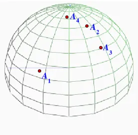
Assume the decision maker chooses to use an additive score function. Following

Notation 3.1, the scores of alternatives can be obtained as (S1, S2, S3, S4) = (0.3, 0.66, 0.45,

0.8). The dissimilarities among alternatives are calculated based on Notation 3.2, as listed in

Table 3.2 (a). Applying Model 3.1 to this example yields the coordinate of each alternative, as

Table 3.1 Data matrix of Example 3.1

ci,k c1 c2 c3 A1 20 100 1.2 A2 35 165 0.8 A3 40 140 0.6 A4 30 180 1 (a) (b) Table 3.2 Results of Example 3.1 with an additive score function

(a) dissimilarity (b) coordinates of alternatives

A1 A2 A3 A4 A1 0.76 0.75 0.70 A2 0.31 0.24 A3 0.55 A4 j i, δ _{x y z} A1 -0.78 0.52 -0.34 A2 -0.40 0.89 0.21 A3 -0.60 0.71 0.37 A4 -0.28 0.96 -0.02

4 A A 2 A 3 A 1

Figure 3.1 The Decision Ball of Example 3.1 with an additive score function

listed in Table 3.2(b). The corresponding Decision Ball is shown in Figure 3.1.

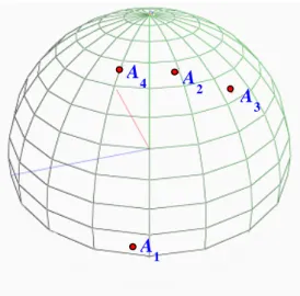
Assume the decision maker selects a multiplicative score function in Example 3.1. From

Notation 3.4, the scores of alternatives are (S1, S2, S3, S4) = (1.06, 4.06, 3.19, 4.45). Based on

Notation 3.5, the dissimilarities among alternatives are calculated, as listed Table 3.3(a).

Applying Model 3.2 to the example yields the coordinates of alternatives, as listed in Table

3.3(b). The Decision Ball with a multiplicative score function is depicted in Figure 3.2.

(a) (b) A1 A2 A3 A4 A1 0.00 1.62 1.67 1.54 A2 0.00 0.00 1.22 1.15 A3 0.00 0.00 0.00 1.40 A4 0.00 0.00 0.00 0.00 j i, δ _{x y z} A1 -0.92 0.06 -0.39 A2 -0.52 0.86 -0.01 A3 -0.61 0.74 0.27 A4 -0.41 0.87 -0.29

Table 3.3 Results of Example 3.1 with a multiplicative score function (a) dissimilarity (b) coordinates of alternatives

A 2 A 3 A A 1 4

Figure 3.2 The Decision Ball of Example 3.1 with a multiplicative score function

3.5 Summary

This section proposes Decision Ball techniques with additive and multiplicative score

functions respectively to provide a useful visual representation of ranks and similarities

among alternatives. An illustrative example is also demonstrated about how to display

Chapter 4 Model 1: Moral Algebra Decision Ball Models

This chapter presents Model 1 – Moral Algebra Decision Ball models for Type I decision

pattern. The decision problems solved in this pattern are Yes/No decision problems. This is

the simplest decision pattern because the decision makers have not to estimate the value of

each criterion for each alternative in advance. Decision makers are assumed to be capable of

making pairwise comparisons between pro and con reasons. Based on Franklin’s Moral

Algebra, this study develops a mechanism to visualize the decision alternatives and processes

on Decision Balls.

The structure of this chapter is organized as follows. Section 4.1 introduces the concept

of Franklin’s Moral Algebra. Section 4.2 constructs Moral Algebra Decision Ball models.

Section 4.3 uses an example to demonstrate how to apply Moral Algebra on Decision Balls.

Summary of this chapter is made in Section 4.4.

4.1 Introduction to Franklin’s Moral Algebra

More than 230 years ago, Joseph Priestly, a noted scientist, asked for advice from

Benjamin Franklin about what option to choose when making a decision. Franklin replied to

his friend that he could not advise what to determine, but would like to tell how. Franklin

success in making rational decisions. (The letter from Benjamin Franklin to Joseph Priestly is

listed in the Appendix)

Franklin thought, the difficulty of making decision was because the reasons pro and con

were not present in the mind at the same time; sometimes one set present themselves, and at

other times another, while the first was out of sight.

Franklin’s Moral Algebra for making choices was first to divide a sheet of paper into

two columns; one for pro, and another for con. Then, write down the various motives, for or

against the choice. Franklin then attempted to estimate the respective weights of these reasons

at one time. If a reason pro equaled a reason con, then both would be crossed out. If a reason

pro equaled two reasons con, the three were crossed out. After a day or two of consideration,

if nothing new came to mind for either side, Franklin would then come to a determination.

Franklin thought that since all the reasons lay before him, and since each reason was

considered separately and comparatively; he could judge better, and was less liable to make a

rash choice. In fact, Franklin benefited a lot from this kind of choice method.

Franklin’s Moral Algebra is an intelligent way of simplifying the complexity of a

decision. By eliminating reasons pro and con step-by-step, the original list of pros and cons

can be replaced with an equivalent but compact list. Then, a clear choice can then be reached.

However, this algebra is not used widely today because of the following facts.

However, it is not easy for a decision maker to tell explicitly which pro(s) and con(s) can be

eliminated simultaneously. Second, the key point in Franklin’s Moral Algebra is to present all

the pros and cons to the mind at the same time, the decision maker therefore can make whole

comparisons about these pros and cons. However, the table listing may not be a proper way to

display complete information to a decision maker. Since a table can only list the items of pros

and cons but can not tell the similarities or differences between them.

This study therefore proposes Moral Algebra Decision Ball models to visualize and

enrich Franklin’s Moral Algebra. The merits of this approach in making choices are listed

below:

(i) The decision maker is not required to directly list equivalent pros and cons. But to

roughly express the comparisons between pros and cons with words such as “equally

important”, “slightly more important”, “more important” and “significantly more

important”.

(ii) After making the comparisons, the differences of importance between pros and cons are

displayed on the surface of a ball. By examining the ball, the decision maker can detect

the closest sets of pros and cons, and then eliminate them simultaneously.

(iii) The whole decision process can now be visualized. By “seeing and choosing”, the

decision maker is more confident when making comparisons, updating preferences,

4.2 Construction of Moral Algebra Decision Ball Models

To illustrate the relationship between pros and cons, we can compare the differences

between them. Suppose an option represents a pro or a con. If two options are equally

important, then the difference of importance between them should be small. If one option is

slightly more important than the other, then their difference becomes larger. If one option is

much more important than the other, then their difference is significantly larger. To visualize

the difference of importance means to convert them into physical distances.

Two rules of allocating all options on the surface of a ball are as follows:

Rule 1 : The more the difference of importance between two options, the longer the physical

distance between them.

Rule 2 : The more important an option is, the closer it is to the north pole.

The decision maker’s preferences between two options A and B are classified and

expressed in Table 4.1.

Preference between A and B Expression

A is equally important as B A ≈ B A is slightly more important than B A _f B A is more important than B A _ff B A is significantly more important than B A _fff B

The essence of Franklin’s Moral Algebra is to simultaneously display the complete

information of pros and cons to the decision maker. This study intends to utilize computer

graphic technologies to develop a decision support system to visualize a decision maker’s

preferences on a ball.

On the surface of a Decision Ball, the distance between two reasons is designed to be the

relationship between them: the more the difference of importance, the longer the distance. The

relationship between relationship type and distance is defined as listed in Table 4.2.

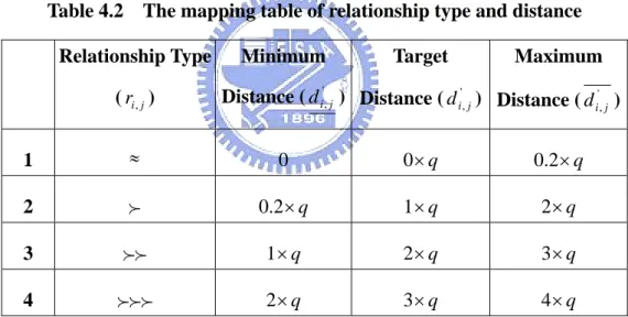
Table 4.2 The mapping table of relationship type and distance Relationship Type (ri,j) Minimum Distance (di', j ) Target Distance (d_i'_{, j}) Maximum Distance (di', j) 1 ≈ 0 0×q 0.2×q 2 _f 0.2×q 1×q 2×q 3 _ff 1×q 2×q 3×q 4 _fff 2×q 3×q 4×q

In Table 4.2, q is a scaling constant, and is the relationship type between two

options i and j. There are four relationship types, including “ j

i r_,

≈”, “ ”, “ ”and “ ”. Each type of relationship is mapped to a target distance , with upper and lower bound

f ff fff ' , j i d ' , j i

d and di', j respectively. Let di,jbe the actual distance between reason i and reason j, and

radius of the Decision Ball be 1. The Decision Ball is formulated as follows:

Model 4.1 A Pro-Con Decision Ball Model

Min  s.t. − ≤di j −di j ≤ ∀ri,j ≠φ , (4.1) ' , , ,  φ ≠ ∀ ≤ ≤ ij ij ij j i d d r d , ' , , ' , , , (4.2) yi ≥ yj +g, if ri,j ∈{"f","ff","fff"}, (4.3) g ≥ g, q≥q, (4.4) (3.13) ~ (3.15),

where g, q are lower bounds of g and q respectively.

The objective is to minimize the difference between the actual distance and target

distance (4.1). Expression (4.2) is used to set the upper and lower bound of di,j. The latitudes

of Pro or Con reasons stand for the order of importance. If a reason Pi is important than Pj, the

latitude of Pi is designed to be higher than that of Pj, as listed in Expression (4.3), where g is a

gap in y coordinate between two reasons with different importance. The lower bounds of g

and q are set in (4.4) in order to avoid all reasons located too close to each other. The suggested values are g = 0.1, q = 0.25.

4.3 An illustrative Example – A CEO’s Dilemma

Here we use an example, called a CEO’s dilemma, to illustrate the process of utilizing a

Decision Ball to assist a manager in making choices.

Imagine a manager, David, who faces a difficult choice. David is the department director

of SOFTCOM, a famous software company with 2000 employees. David came to the U.S.A

from Shanghai, China. After obtaining his PhD from Wharton business School, David was

recruited by SOFTCOM. Because of his outstanding ability in analysis, he has been promoted

to a senior position in SOFTCOM. David has a lovely family, his wife Lisa and two children

Ivy and Paul. Ivy is 10 and Paul is 6.

Because of the boom in the Chinese market, SOFTCOM plans to establish a subsidiary

in Shanghai. One week ago, David was asked to be the CEO of the China subsidiary of

SOFTCOM. The rewards of this new position are quite promising. The salary will be doubled,

and David may be promoted to the Asia’s director of SOFTCOM in the future. In addition,

David can take care of his old parents in Shanghai. However, Lisa, Ivy and Paul do not want

to leave. After staying at home for 5 years to take care of kids, Lisa cherishes her current job.

Ivy and Paul love their current schools very much. In addition, Ivy and Paul cannot speak

Chinese and may not make many friends in China. David is very excited about the new

position; however, he does not want to be separated from his family. David needs to choose

this week. How can he make this decision?

since all of these tools ask David to specify explicitly the trade-offs between “job and family”

or between “money and love”. David does not like it. Now we assist David to make his

decision via a Decision Ball.

There are five steps of making a choice:

Step 1 Listing of Pros and Cons

Suppose David lists five pros in order of importance (roughly) for accepting the new

position. First, this is a great promotion opportunity. If he accepts this new position, it is very

possible he will be promoted to be the director of Asia in three years. Second, David’s parents

live in Shanghai. Both of them are over 75 years old. He can give his aging parents attention

if he moves back to China. Third, the salary of the new position is more than twice as high as

his salary now. Fourth, to be the CEO of a Chinese subsidiary, he could make more

contributions to his homeland. Last, David has an aggressive personality and likes a career

that offers a challenge. To be a CEO of Chinese subsidiary is an exciting challenge for him.

David also lists five cons in order of importance (roughly). First, both kids were born in

the U.S.A. They cannot speak Chinese. They may have a tough time transforming to a new

culture. Besides, both kids enjoy their American-style school life very much and object to

leaving. Second, David’s wife is an accountant. Lisa has worked hard and has recently got a

promotion to section manager. She is not willing to quit her job. Third, the population density

a new house in the U.S.A. one year ago. The house has a great view and a beautiful yard. The

family likes the house very much and they are not willing to move out. Finally, David and

Lisa have lived in the U.S.A. for over 16 years. Most of their friends are in the U.S.A. They

cherish their friendships very much.

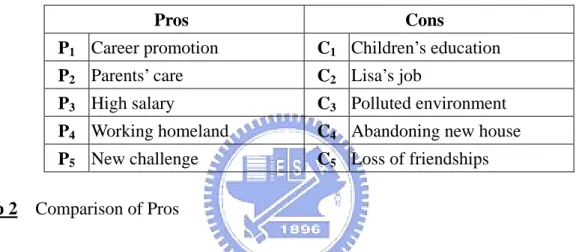
The summary of pros and cons are listed in Table 4.3.

Table 4.3 David’s list of pros and cons for accepting the new position

Step 2 Comparison of Pros

David selects some pros for comparison, as listed in Figure 4.1(a).

Comparing Career promotion (P1) with other pros, David thinks career promotion is

equally important as Care for parents (P2), more important than High salary (P3), more

important than Working for the homeland (P4), and significantly more important than a

New challenge (P5). These preferences are expressed as P1≈P2, P1ffP3, P1ffP4, and

P1fff

f

Pros Cons

P5.

P1 Career promotion C1 Children’s education

P2 Parents’ care C2 Lisa’s job

P3 High salary C3 Polluted environment

P4 Working homeland C4 Abandoning new house

P5 New challenge C5 Loss of friendships

Comparing Parents’ care (P2) with other pros, David thinks itis slightly more important

compared to a High salary (P3) as well as Working for homeland (P4), denoted as P2fP3

P1 P2 P3 P4 P5 P1 : Career promotion ≈ ff ff fff P2 : Parents’ care f f P3 : High salary _f P4 : Working homeland ff P5 : New Challenge P5 P4 P3 P2 P1

Figure 4.1 Pro Ball of Example 4.1 (a) Relationships among pros (b) David’s Pro Ball

(a) (b)

≈: equally important; f: slightly more important;

ff: more important; _fff: significantly more important.

Comparing High salary (P3) with other pros, David is unclear about the comparison of

High salary (P3) and Working for homeland (P4). What he can sure is High salary (P3) is

slightly more important than a New challenge (P5 ) (P3fP5). Working for homeland (P4)

seems more important than a New challenge (P5) (P4ffP5).

After David finishes filling out preferences in Figure 4.1(a), the Decision Ball system

then maps David’s preferences into a Pro Ball in Figure 4.1(b). Figure 4.1(b) illustrates the

relationships among the five pros. The arc length between two pros indicates their differences

of importance: the longer the distance, the larger the difference. For instance, because the

importance of Career promotion (P1) over a New challenge (P5) is higher than that of Career

promotion (P1) over High salary (P3), the distance between P1 and P5 is much longer than that

of P1 and P3. Moreover, the latitude of a pro stands for the order of importance. For example,

latitude of P1 is much higher than P5.

Figure 4.1(b) shows that Career promotion (P1) and Parents’ care (P2) are the closest to

each other, and Career promotion (P1)and a New challenge (P5) are the longest distance apart;

which fit the preference values in Figure 4.1(a). It is noteworthy that High salary (P3) and

Working for homeland (P4) are close to each other, which implies P3 and P4 may be of similar

importance. This relationship was not realized by David before; but it is visually illustrated by

the ball. Moreover, David could also choose to revise the relationship between pro reasons in

Figure 4.1(a) to modify his Pro-Ball iteratively.

Step 3 Comparison of Cons

David selects some cons for comparisons, as listed in Figure 4.2(a).

Considering his Children’s education (C1), it seems slightly more important than Lisa’s

job (C2) (C1fC2), because David thinks Ivy and Paul can only have a childhood once.

C1 C2 C3 C4 C5 C1: Children’s education f f fff C2 : Lisa’s job _f C3 : Polluted environment ff C4 : Abandoning new house ff C5 : Loss of friendships C4 C5 C3 C2 C1

Figure 4.2 Con Ball of Example 4.1(a) Relationships among con reasons (b) David’s Con Ball

(a) (b)

≈: equally important; f: slightly more important;

His children’s education is slightly more important than a Polluted environment (C3), and

is significantly more important than Loss of friendships (C5) (C1fC3, C1fffC5).

Lisa’s job (C2) is slightly more important than Abandoning their new house (C4).

Both a Polluted environment (C3)and Abandoning new house (C4) are more important

than the Loss of friendships (C5).

A Con Ball associated with Figure 4.2(a) is depicted in Figure 4.2(b).

Step 4 Comparison between Pro(s) and Con(s)

Next, David needs to specify the relationship between pro and con reasons, as listed in

Figure 4.3(a).

Since Lisa had stayed at home for 5 years to care for the kids before she got her current job, the job means a lot to her. David therefore thinks his Promotion opportunity (P1) is

equally important as Lisa’s job (C2).

It is difficult to compare Care for parents (P2) with any con. David therefore does not

make any comparison here.

Working for homeland (P4) is equally important as the problems caused by a Polluted

environment (C3).

David thinks his family’s emotional reluctance to Abandon their new house (C4) is

slightly more important than the pleasure due to a Higher salary (P3), denoted as P3pC4.

which merges the Pro-Ball in Figure 4.1(b) and the Con-Ball in Figure 4.2(b). During the

merging process, the system reallocates all pros and cons in order to let Career promotion (P1)

and Lisa’s job (C2), Working for homeland (P4) and a Polluted environment (C3) be as close as

possible, to let the latitude of Abandoning the house (C4) be higher than that of a High salary

(P3). This is because David feels P1≈C2, P4 ≈C3, and P3 pC4, as specified in Figure 4.3(a).

Step 5 Swapping Equivalent Pros and Cons

By examining the Pro-Con Ball in Figure 4.3(b), David finds that Career promotion (P1)

and Lisa’s job (C2) are very close to each other, that means P1 and C2 are equally important

(as specified in Figure 4.3(a)); therefore, P1 and C2 can be eliminated (marked with a dash

oval in Figure 4.3(b)). Similarly, a Polluted environment (C3) and Working for homeland (P4)

can be eliminated. It is worthy to notice that Loss of friendships (C5) and a New challenge (P5)

are also close to each other, which means they may be of similar importance although David

did not realize it in Figure 4.3(a). This can only be visualized on a ball. Suppose David

decides to eliminate a New challenge (P5) and the Loss of friendship (C5). The final Decision