求解離子通道之二階Poisson Nernst-Planck簡化法

國立交通大學

應用數學系

碩 士 論 文

求解離子通道之

二階 Poisson Nernst-Planck 簡化法

A simplified second-order Poisson Nernst-Planck solver for ion channel

研 究 生: 楊祥鶴

指 導 教 授 : 劉晉良 博士

共同指導教授 : 吳金典 博士

求解離子通道之二階 Poisson Nernst-Planck 簡化法

A simplified second-order Poisson Nernst-Planck solver

for ion channel

研 究 生 : 楊祥鶴 Student : Shiang-He Yang

指 導 教 授 : 劉晉良 博士 Advisor : Jinn-Liang Liu

共同指導教授 : 吳金典 博士

Co-advisor : Chin-Tien Wu

國立交通大學

應用數學系

碩 士 論 文

A Thesis

Submitted to Department of Applied Mathematics

College of Science

National Chiao Tung University

in Partial Fulfillment of the Requirements

for the Degree of

Master

In

Applied Mathematices

June 2012

求解離子通道之二階 Poisson Nernst-Planck 簡化法

學生:楊祥鶴 指 導 教 授 : 劉晉良

共同指導教授 : 吳金典

國立交通大學應用數學系（研究所）碩士班

摘要

本論文運用基本的 Poisson Nernst-Planck(PNP)數學模型來模擬生物細胞的離子通 道在穩定狀態的情形,然而 Poisson 方程式可經由庫倫定律和高斯定理來獲得,至 於 Nernst-Planck 方程式則是等價於漂移擴散數學模型,過去很多的計算方法都已 經被應用在 PNP 數學模型上,然而我們的主要目的是去簡化在[24]裡面的計算方 法,並且保持二階收斂的效果,但我們有一些必須要去處理的問題,例如我們應用 位能分解方法[5]去處理 Delta 函數,使用合適的介面和邊界(matched interface and boundary)方法 [24]來處理不同介質的問題,而對於初始值猜測則必須由 Poisson Boltzmman 方程得到,最後我們由分子資料銀行(protein data bank)得到真實的短杆 菌肽(Gramicidin A)通道的資訊並且建構它的幾何結構。

A simpli…ed second-order Poisson Nernst-Planck

solver for ion channel

Student: Shiang-He Yang

1

Advisor: Jinn-Liang Liu

2

, Chin-Tien Wu

1

1

_{Department of Applied Mathematics}

National Chiao Tung University

2

_{Department of Applied Mathematics}

National Hsinchu University of Education

July 3, 2012

Abstract

The Poisson-Nernst-Planck (PNP) model is a basic continuum model for sim-ulating ionic ‡ows in an open ion channel. It is one of commonly used models in theoretical and computational. The Poisson equation is derived from Coulomb’s law in electrostatics and Gauss’s theorem in calculus. The Nernst-Planck equation is equivalent to the convection-di¤ussion model. Many computation methods have been constructed for the solution of the PNP equations. However, we want to sim-plify the second order solver of proposed in the literature [24] but, we must to deal with some problems. For example, singular charges, nonlinear coupling and inter-face. First, we apply the decomposition method [5] proposed by Chern, Liu and Wang to cope with the singular charges. Second, the matched interface and bound-ary (MIB) method [24] is used for the interface problem. Third, the initial guess are given by Poisson Boltzmann (PB) equation and two iterative schemes are utilized to deal with the coupled nonlinear equations. Finally, the real data of Gramicidin A (GA) channel protein is obtained from the protein data bank (PDB).

誌謝

本篇論文的完成,首先感謝我的指導老師劉晉良博士,在這二年間的悉心教誨,而 劉老師雄厚的物理知識以及在半導體上的豐富經驗,也幫助我運用在生物系統上 解決了很多的問題,在此獻上我最誠摯的感謝。另外也感謝我的共同指導老師吳 金典博士,老師所教授的有限元素方法用途非常的廣而理論架構也相當完整,我相 信對我的未來發展一定有相當大的幫助。 同時感謝我的口試委員陳人豪教授和彭振昌教授，於口試期間的建議以及對疏漏 處的提醒和指正。 而在交大應數的這兩年，無論是在課堂上，亦或是參與各種演講和研討會，都讓 我學習到做研究的精神與態度，在此感謝所有我修過課的老師們以及我所參加過 的演講的所有教授們。再來我要感謝所有在碩班認識的同學、學長姐和學弟妹。 以及在系壘認識的各位，在我的研究生生涯中，因為有你們的陪伴，我的生活才 得以充實，充滿歡笑與快樂，謝謝你們。 在這邊，我要特別感謝我的家人以及女友，一直在背後支持、陪伴和鼓勵著我， 謝謝爸爸和媽媽提供給我很好的環境和資源，讓我在我的學生生涯能夠無後顧之 憂，在我的求學的路上也沒有給我任何壓力，並尊重我做的任何決定。能夠順利 完成這篇論文，這份榮耀我要與你們分享，也希望我能成為你們的驕傲。 楊祥鶴 謹誌于交通大學 2012 年六月

Contents

1 Introduction 3

2 Poisson-Nernst-Planck model and numerical methods 4

2.1 Poisson-Nernst-Planck model . . . 5

2.2 Numerical methods for PNP . . . 8

2.2.1 Finite di¤erence method for Poisson’s equation . . . 8

2.2.2 Matched interface and boubdary method (MIB) . . . 9

2.2.3 FDM for Nernst-Planck (NP) equation in primitive form . . . 12

2.2.4 The Decomposition of electrostatic potential . . . 15

2.2.5 The Gummel and SOR-Like schemes . . . 17

2.3 Test case for PNP equations . . . 17

3 The Poisson-Boltzmann (PB) equation 18 3.1 The Poisson-Boltzmann (PB) equation and linearization . . . 19

3.2 Monotone iterative method for the nonlinear PB equation . . . 21

4 Dimensionless formulation and approximation of interface condition 23 4.1 Unit Conversion and physical constants . . . 23

4.2 Dimensionless formulation . . . 24

4.3 Approximation of interface conditions . . . 30

4.4 Numerical results for test cases . . . 33

1

Introduction

Biological ion channel is a porous protein on cell membrane and they are present in the membranes that surround all biological cells. It allows some particular ions across cell membrane and then controls the electrical potential di¤erence of the internal and exterior part. These ions move through the channel pore single …le nearly as quickly as the ions move through free ‡uid. In some ion channels, passage through the pore is governed by a "gate" which may be opened or closed by chemical or electrical signals, temperature, or mechanical force..., depending on the variety of channel. Ion channel is vary important for process of life such as control hormone ooze, preservation of salt and water balance, sensory transduction, nerve and muscle excitation, muscle contraction etc. [13], in general, ion channels may be classi…ed by the nature of their gating, species of ions passing through those gates or the number of gates (pores) and localization of proteins. Moreover, ion channels may be classi…ed by gating, i.e., what opens and closes the channels. For example, voltage-gated ion channels open or close depending on the voltage gradient across the plasma membrane, while ligand-gated ion channels open or close depending on binding of ligands to the channel.

The following is some of the most important development of ion channels, British biophysicists Alan Hodgkin and Andrew Huxley discoveries concerning "the ionic mech-anisms in the nerve cell membrain" (Nobel Prize in Physiology or Medicine 1963), Erwin Neher and Bert Sakmann discoveries concerning "the function of single ion channels in cells" (Nobel Prize in Physiology or Medicine 1991). Roderick MacKinnon for his stud-ies on the physico-chemical propertstud-ies of ion channel structure and function, including x-ray crystallographic structure studies, and Peter Agre for his similar work on aquapor-ins (Nobel Prize in Chemistry 2003). In the past decades many experimental techniques have been well-developed for study ion channels [14]. However, this data has driven the development of the theory and calculations. The commonly used method are ab initio molecular dynamics (MD) and classical molecular dynamics (MD) [19]. Because taking into account each ion, it requires a very large number of computing.

The Poisson-Nernst-Planck (PNP) equations are an approximation of ions, for which we do not deal with a discrete distribution for the ions. Instead, we consider continuous charge densities. The PNP theory considers the real channel structure and discrete protein charge locations in its modeling and computation. The PNP theory neglects the …nite volume e¤ect of ion particles, which can be important for small channel pores [16]. The existence and uniqueness of PNP equation is an important issue in mathematics and on certain restrictions can be obtained [2][3][10]. Due to the overly complex domain, analytic solution to the original PNP system is unfeasible. Therefore, we focus on the numerical solution and thus understand the meaning of the results. PNP is a very interesting

model that includes three coupled equations, irregular geometry, discontinuous dielectric coe¢cients, singular charges and nonlinearity.

In mathematics, a lot of discrete methods have been used to solve the PNP equation, such as …nite dii¤erence method, …nite element method, …nite volume method and spectral element method. Among them Q. Zheng, D. Chen and G. W. Wei provide a second-order convergeence method [24] and this is …rst method that yields a second-order convergence in the literature for three-dimensional (3D) realistic geometry of the Gramicidin A(GA) channel, but the method requires up to 27 …nite di¤erence points. We simplify this di¤erence method to seven points formula and maintain the quadratic convergence. For initial guess, the potential is obtained by Poisson-Boltzmann (PB) [23] equation and it is a nonlinear equation. The PB equation will be solved by linearized PB equation as initial guess and then will need to implement monotone iterative method [17] to solve nonlinear PB equation. For the singular charge, we implemant the decomposition method proposed by Chern, Liu, and Wang [5] and the potential is decomposed into three parts such that delta function disappears in the right hand side. Because we use this decomposition method [5], we must approximate the gradient of the Green function (section 2.2.4 and 4.3). For interface problem, the match interface and boundary (MIB) method is used to connect solvent and molcular parts and to treat jump conditions.

For channel structure, Visual Molecular Dynamics (VMD) [15] is designed for model-ing, visualization, and analysis of biological systems such as proteins, nucleic acids, lipid bilayer assemblies, etc. It may be used to view more general molecules, as VMD can read standard Protein Data Bank (PDB) …les and display the contained structure. VMD can be used to animate and analyze the trajectory of a molecular dynamics (MD) simulation. In particular, VMD can act as a graphical front end for an external MD program by displaying and animating a molecule undergoing simulation on a remote computer. We consider water in the channel and generate Molecular Surface (interface) in 3D uniform grid by van der Waas radii and a probe ball, i.e., closest distance of water molecules with protein that is obtained by VMD.

2

Poisson-Nernst-Planck model and numerical

meth-ods

Biological ion channels seem to be a precondition for all living matter [20]. Ion channels are porous proteins across cell membranes that control many biological functions rang-ing from signal transfer in the nervous system to regulation of secretion of hormones. Understanding the mechanism of ionic ‡ows within a channel as a function of ionic con-centration, membrane potential, and the structure of the channel is a central problem in

molecular biophysics [12]. The PNP model proposed by Eisenberg and coworkers [8][9] as a basic continuum model for simulating the ionic ‡ow in an open ion channel is one of commonly used models in theoretical and computational studies of biological ion channels.

2.1

Poisson-Nernst-Planck model

For modeling the ‡ow of two species of ions through a channel, the steady-state PNP model (2.1.1)-(2.1.3) reads as [24] P : _{¡r ¢ (()r()) = 4}  X =1 (¡ ) + 4 2 X =1 () 2 ­ (2.1.1) NP1 : _{¡r ¢ }1() = 0  2 ­ (2.1.2) NP2 : _{¡r ¢ }2() = 0  2 ­ (2.1.3) _() = _¡() [_r() + __()_{r()] for i = 1, 2} (2.1.4) ¤() = 4  X =1 (¡ )¼  X =1   p (_{¡ })2+ (¡ )2+ (¡ )2 (2.1.5)

where  = (  ), () is the current density of an ion species  with , () is

the concentration of an ion species  carrying charge  (for example,+ = +1 _¡ =

¡1),  the concentration ‡ux (current density),  the spatially dependent di¤usion

coe¢cient, _ = ( ),  the Boltzmann constant,  the absolute temperature,  the

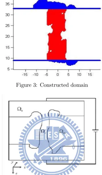
electrostatic potential,  the dielectric constant , and  the protein charge. The domain ­ = ­ [ ­ consists of two subdomains, namely, the solvent subdomain ­ and the

biomolecular subdomain­. The electric permittivity has di¤erent values in subdomains

and denoted by () =  = ½ 8 2 ­ __{8 2 ­} ¾ (2.1.6) where  = is the dielectric constant of the solvent, and  = is the dielectric constant

of the molecules. We consider the domain as a cubical box

Box = ­ = (¡20 º 20 º)_{£ (¡20 º} 20 º)_{£ (0 º} 40 º) (2.1.7) For the jump condition at the interface ¡ given by

Poisson equation: [()] = +_{¡ }¡ = 0 _{2 ¡} (2.1.8) [()_()] = r+¢  ¡ r¡¢  = 0  2 ¡ (2.1.9) Nernst-Planck: _()_{¢  = 0  2 ¡} (2.1.10) where ¡ = ­\ ­ (2.1.11) + = lim !+()  ¡_{= lim} !¡()  ¡ _{2 ­}  + 2 ­ (2.1.12)

¡ is the interface set between ­ and ­,  is an outward normal unit vector on ¡ and

º

 is equal to 10¡8_{().}

Figure 1: VMD simulation system of the KcsA channel with membrane, water,and ions.

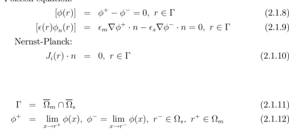
Figure 3: Constructed domain

Figure 4: A cross section of 3D PNP simulation domain for GA channel.

Fig. 4 is across section of 3D PNP simulation domain for the GA channel [7]. Fig. 2 is a side view of the GA channel embedded in the membrane [24]. Fig. 1 illustrates a VMD [15] simulation system of the KcsA channel with membrane, water, and ions [1]. The channel protein is in the central part of the simulation domain (a box) as shown in green color. The membrane consists of bilipid layers shown in light blue surrounding the channel. The upper and lower regions represent the extracellular (outside of a cell) and intracellular (inside) solvent regions, respectively, that consist of water and ions.

2.2

Numerical methods for PNP

2.2.1 Finite di¤erence method for Poisson’s equation

Discretization of the left hand side of (2.1.1) by the central …nite di¤erence method (FDM) yields ¡  (() (  )  )¼ ¡¡12¡1+ (¡ 1 2 + + 1 2)¡ + 1 2+1 ¢2 (2.2.1)

for all (  )2 ­[ ­ ()_ =   = (  ) ¢ = ¡ ¡1 = , and  are

…nite di¤erence grid points. We assume a uniform partition of the box in each direction, i.e., ¢ = ¢ = ¢ = . To simplify the notation, we write (2.1.1) in 1D as

¡_ (()()

 ) =  (2.2.2)

The second-order, denoted by O(h2_{) (convergence order is 2), central FD approximation}

of (2.2.2) is ¡¡12¡1+ (¡ 1 2 + + 1 2)¡ + 1 2+1 ¢2 =  (2.2.3)

For interface problem, we alway assume that

_¡1   = _¡1

2   (2.2.4)

i.e., every jump position  2 ¡ is at the middle of some neighboring grid points. We consider the following jump condition for Poisson problem (2.1.8) (2.1.9)

[()] = +_{¡ }¡ = 0_{,  2 ¡} (2.2.5) [()_()] = _r+_{¢  ¡ r}¡_{¢  = 0,  2 ¡} (2.2.6) For the jump condition in 1D, we have

[()_()] = r+¢  ¡ r¡¢  = + ¡ ¡,  = (1 0 0) (2.2.7)

or

[()_()] = _r+_{¢  ¡ r}¡_{¢  = ¡}+_ + _¡_{,  = (¡1 0 0)} (2.2.8) Remark. 2. 1: By (2.1.8) and (2.1.9), it is easy to observe that the electrostatic potential

2.2.2 Matched interface and boubdary method (MIB)

For di¤erent dielectric constant ,  and the non-di¤erential point, the MIB is used to

deal with this problem such that we can obtain a second-order convergence formula. The main ideas of the MIB method for handling the jump problem are

(1) considering (2.2.2) as two di¤erent subproblems with two disjoint subdomain    and   ,

(2) taking the jump condition (2.2.5) and (2.2.6) as the boundary conditions for each subproblem with respect to its subdomain,

(3) extending smoothly a function () de…ned on a subdomain to a ‘…ctitious’ func-tion ª() de…ned on another subdomain, and

(4) applying Taylor’s theorem to the jump conditions for joining two subproblems back to one.

De…ne the extension functions

 () =_f()_{ª(), if ¸}, if _{or () = f}()_{ª(), if ·}, if  (2.2.9) Applying Taylor’s theorem to  () at the interface, we have

 (_¡1) =  () + 0()(_{¡1 ¡ ) +} 0_() 2! (¡1 ¡ ) 2_{+ (}3_{) (2.2.10)}  () =  () + 0()(¡ ) + 0() 2! (¡ ) 2_{+ (}3_{) (2.2.11)}  () =  (¡1) +  () 2 + ( 2_{) (2.2.12)}

Hence, for (2.2.5) we have

¡ =  () = ¡1+ ª 2 + ( 2_{) (2.2.13)} + = () = + ª¡1 2 + ( 2_{) (2.2.14)} [] = + ª¡1 2 ¡ _¡1+ ª 2 + ( 2_{) (2.2.15)}

0() =  ()¡  (¡1) + (3) (2.2.16) ¡_ = 0() = ª¡ ¡1  + ( 2_{) (2.2.17)} +_ = 0() = ¡ ª¡1  + ( 2_{) (2.2.18)} [_] =  _{¡ ª¡1}  ¡  ª¡ _¡1  + ( 2_{) (2.2.19)}

Therefore, by (2.2.15) and (2.2.19), the following equations

1_¡1+ 2ª = 3ª¡1+ 4¡ [] (2.2.20)

¡(1_¡1+ 2ª) = +(3ª¡1+ 4)¡ [] (2.2.21)

represent FD approximations of (2.2.5) and (2.2.6), respectively, with local truncation errors of (2_{)Here, the weight are}

1 = 2 = 3 = 4 = 1 2 (2.2.22) 1 = 3 = ¡1   2= 4 = ¡1  (2.2.23)

Solving (2.2.20) and (2.2.21) for the …ctitious values ª_and ª_+1 we obtain ª_¡1 = ( ¡_ 21¡ +12)_¡1 ¡ (¡24¡ +42) ¡_{23¡ }+_ 32 + ¡_ 2[]¡ 2[] ¡_{23¡ }+_ 32 = 1_¡1+ 2+ 0 (2.2.24) ª = ¡( +_ 31¡ ¡13)_¡1+ (+34¡ +42) +_ 32 ¡ ¡23 +¡ +_ 3[] + 3[] +_ 32¡ ¡23 = 1_¡1+ 2+ 0 (2.2.25)

Following (2.2.3) by di¤erencing  () at the grid point _¡1 and di¤erencing () at the grid point , we obtain

¡¡32¡2+ (¡ 3 2 +  ¡ ¡12 )_{¡1¡ }¡ ¡12 ª+1 ¢2 = ¡1 (2.2.26) ¡+_¡1 2 ª_¡1+ (+ ¡12 + _+1 2)¡ + 1 2+1 ¢2 =  (2.2.27)

Although ª and ª¡1 are called …citious (ghost) value, they are real in implemantation

and de…ned by (2.2.24) (2.2.25) via _¡1 and _. Consequently, (2.2.26) and (2.2.27) become ¡¡32¡2+ (¡ 3 2 + (1¡ 1) ¡ ¡12 )_{¡1¡ }2¡_¡1 2 _ ¢2 = ¡1+ ¡ ¡12 0 ¢2 (2.2.28) ¡1+_¡1 2 _¡1+ ((1_{¡ }2)+_¡1 2 + _+1 2)¡ + 1 2+1 ¢2 = + + ¡1 2 0 ¢2 (2.2.29) or (by  = _¡1 2) ¡_¡2+ (+ (1¡ 1))_¡1¡ 2 ¢2 = ¡1+ 0 ¢2 (2.2.30) ¡1_¡1+ ((1¡ 2)+ )¡ +1 ¢2 = + 0 ¢2 (2.2.31) ¡1_¡1 + ((1¡ 2)+ ) ¡ +1 ¢2 +¡1¡1+ ((1¡ 2)+ ) ¡ +1 ¢2 = _+0 ¢2 + 0 ¢2 (for 2 jumps in 2D) (2.2.32) whewe 1 = (¡21¡ +12) ¡_{23¡ }+_ 32 = 2¡ 1 2 ¡ 3 = 2 +  (2.2.33) 2 = ¡( ¡_ 24¡ +42) ¡_{23¡ }+_ 32 = ¡2+ 4 2¡ 3 = ¡  +  (2.2.34) 0 = ¡_ 2[]¡ 2[] ¡_{23¡ }+_ 32 = 22[]¡ [] 2¡ 3 = 2[]¡ [] +  (2.2.35) 1 = ¡( +_ 31¡ ¡13) +_ 32¡ ¡23 = ¡(3 ¡ 1) 3¡ 2 = ¡(¡ ) +  (2.2.36) 2 = (+_ 34¡ +42) +_ 32¡ ¡23 = 3¡ 4 3 ¡ 2 = 2 +  (2.2.37) 0 = ¡ +_ 3[] + 3[] +_ 32¡ ¡23 = ¡23[] + [] __{3¡ }₂ = ¡2[]¡ [] _+ _ (2.2.38)

For = 1, = 80, and [] =0, we have 1 = 2_{¢ 80} 81  2 = ¡79 81  0 = ¡[] 81  1¡ 2 = 2_{¢ 80} 81  (2.2.39) 1 = 79 81 2= 2 81 0 = ¡[] 81  1¡ 2 = 2 81 (2.2.40)

which lead to a diagonally dominant matrix from (2.2.30) and (2.2.31). By (2.2.20) and (2.2.21), we introduce two unknows ª_¡1 and ª_ in order to treat the two jump condition [] and []. If [] = 0, we actually have only one jump condition [] to take care of. Hence, we should let either ª=  or ª¡1= ¡1 in (2.2.21). If we let ª= , then

(2.2.20) become

1_¡1 = 3ª¡1¡ [] (2.2.41)

which means that the …ctitious value ª_¡1 will cause an (2_{) error to approximate []}

if (2.2.27) is in use. The next question is from which of (2.2.30) and (2.2.31) we should choose. Numerical results show that (2.2.31) is better. Nevertheless, if both [] 6= 0 and [_{] 6= 0we should use both.}

2.2.3 FDM for Nernst-Planck (NP) equation in primitive form

We …rst consider the NP equation in the primitive form, and simplify it in 1D as ¡_ =   µ·  µ   +    ¶¸¶ =  = 0 (2.2.42) Di¤erencing (2.2.42) at x gives ¡ (_  ) ¼ ¡+ 1 2 ¡ ¡ 1 2 4 (2.2.43) ¡+1₂ ¼ ·  µ   +    ¶¸ +1₂ (2.2.44) ¼ · _+1 2 µ +1¡  4 + + 1₂ +1+  2 _{+1¡ } 4 ¶¸ (2.2.45) ¡¡12 ¼ · _¡1 2 µ ¡ ¡1 4 + ¡12 + ¡1 2 _{¡ ¡1} 4 ¶¸ (2.2.46) ¡ (_  ) ¼ 1 42[¡1¡1+ + +1+1] (2.2.47)

_¡1 = _¡1 2 ¡ ¡ 1 2¡12 (_{¡ ¡1})2 (2.2.48)  = ¡(_¡1 2 + + 1 2)¡ ¡ 1 2¡12 (_{¡ ¡1})2 (2.2.49) +_+1 2+ 1₂(+1¡ )2 (2.2.50) +1 = +1₂ + +1₂_{+ 1} 2 (_{+1 ¡ })2 (2.2.51) _¡1_¡1+ + +1+1 42 =  (2.2.52)

where equation (2.1.10) is a boundary condition for Nernst-Planck problem not an in-terface condition. Moreover it is usually called the Robin boundary condition since it involves the data of both the unknown  itself and r. If a boundary condition is in terms of  only, it is then called a Dirichlet boundary condition and is called Neumann boundary condition if in terms of r only. By (2.1.10), we write in 1D as

_{¢  =  ¢ h1 0 0i = }  = _¡(

 +  

) = (= 0 in real equation) at  (2.2.53)

We discuss the …nite di¤erence approximation of (2.1.10) in two case. Case 1. _{n = h1 0 0i, x¡1 2 ­}, x_{ 2 ­}, x_¡1 2 = . Let _¡ 1 2 =_¡ · (  +   ) ¸ ¡12 (2.2.54) Finite di¤erence approximation of (2.1.10) at x_¡1

2 =  is µ ¡¡12 ª¡ ¡1 4 ¡ ¡12  ¡12 ª + ¡1 2 _{¡ ¡1} 4 ¶ = _¡1 2 (2.2.55)

where ªis a …ctitious value. We extend the function () continuously from x¡1 to x by

considering ª as an extra unknown that approximates the ghost value (). This  FD

equation and the  ¡ 1 _{equation (2.2.52) across the interface can be written respectively}

as ª+ ¡1¡1 = ¢ ¡12 (2.2.56) _¡2_¡2+ _¡1_¡1+ _ª_ ¢2 = ¡1 (2.2.57)  = ¡_¡1 2 ¡ ¡ 1 2¡ 1 2 ¡ _{¡ ¡1}¢2 (2.2.58) _¡1 = _¡1 ¡  ¡1¡1 ¡ _{¡ ¡1}¢2

Case 2. n=_{h¡1 0 0i , } 2 ­, +1 2 ­, and  = +1₂. Similarly, we have ª+ +1+1 = ¢ +1₂ (2.2.59) ª+ +1+1+ +2+2 ¢2 = +1 (2.2.60)  = ¡+1₂ + +1₂+1₂ ¡ _{+1¡ }¢2 (2.2.61) +1 = +1 2 + + 1 2+ 1 2 ¡ _{+1¡ }¢2

Now we will introducing the Slotoom variable b [22] by

_ = b_exp(_¡) (2.2.62) the concentration ‡ux is then reformulated to

J =¡exp(¡)r b =¡r b  = exp(¡) (2.2.63)

Consequently, the self-adjoint PNP is ¡r ¢ (r) = 4  P =1 (r¡ r) + 4 2 P =1  (2.2.64) ¡r ¢ J =r ¢ h r b i = 0,  = 1 2 (2.2.65) Consider the Slotboom form of NP (2.2.65) with (2.2.62) and (2.2.63). In 1D, it reads as

¡_ =   Ã  b  ! =  (2.2.66)

and the FD equation at  =  is

_¡1 2b¡1¡ ³ _+1 2 + ¡ 1 2 ´ b + +1₂b+1 ¢2 = . (2.2.67)

Corresponding to (2.2.53) and (2.2.55), we have respectively

 =_¡ b  =  at  (2.2.68) ¡¡12 b ª¡ b¡1 ¢ = ¡12 (2.2.69)

Eq. (2.2.68) is a Neumann BC. If a Dirichlet BC is considered, we then have b

 = _b at  =) bª =b or (2.2.70)

 = , ª =  (primitive).

The method (2.2.55) (or (2.2.69)) alone to treat the Robin (or Neumann) BC is usually unstable due to many unde…ned normal vectors n at corner points. To stabilize the method, we make connections between the adjacent points of ª and ª¡1. For this, in

addition to (2.2.55), we impose

¡ª + ª₂ ¡1 = _¡¡1

2 (2.2.71)

¡ª + ª¡1 = 0, if ¡1

2 is not given.

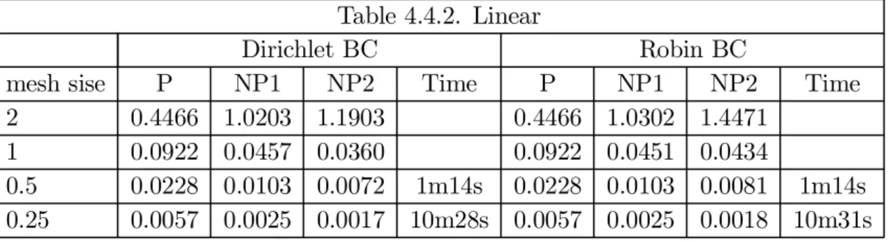
All Robin (with stabilization for the primitive form), Neumann (with stabilization for the Slotboom form), and Dirichlet BCs are implemented for both GA and cylinder. On the interface ¡, we should use either Robin or Neumann BCs. Dirichlet BCs are used only for testing the code. All numerical results are good as shown in the following tables. 2.2.4 The Decomposition of electrostatic potential

We now implement the decomposition method proposed by Chern, Liu, and Wang [5] to cope with the singular charges obtained from the protein data bank (PDB). By this method, the potential (r) is decomposed into

(r) = e(r) + (r) r _{2 ­ = ­}[ ­ ¡ = ­\ ­ (2.2.72) such that (r) = ½ ¤(r) + 0(r)_{, r 2 ­} 0_{, r 2 ­}n¡ , e(r) = ½ _{¡ }¤_{¡ }0_{, r 2 ­}  r _{2 ­}n¡ (2.2.73) ¡r ¢³_re´ = 4 2 P =1  r2 ­n¡ (2.2.74) ¡¢ = ¡¢¤¡ ¢0 r2 ­ (2.2.75)

and the Poission equation of 0 given by ½

¡¢0(r) = 0 r 2 ­

0(r) =_¡¤ r_{2 ­}

(2.2.76) and ¤ is the Green function given analytically

¤(r) =  P =1   p (_{¡ })2+ (¡ )2+ (¡ )2  r_{2 }3 (2.2.77) which is the fundamental solution of the following equation

¡¢¤(r) = 4 

P

=1

(r¡ r) r2 3. (2.2.78)

Summing (2.2.74), (2.2.75), and (2.2.79) gives

¡r ¢ (r) = ¡r ¢³_r(e + )´=_{¡r ¢}³_re´_{¡ }¢¤¡ ¢0 = 4  P =1 (r¡ r) + 4 2 P =1  r2 ­n¡. (2.2.79)

which is exactly (2.1.1). Note that ¤ satis…es (2.2.79) in the whole space 3 _{of a uniform}

medium with the dielectric constant . Since we have two di¤erent media of  and 

in a bounded domain ­, 0 can be thought as a correction potential to ¤ that accounts the electric responses of di¤erent dielectrics and boundary conditions. In general, the analytical form of 0 is not available and hence its numerical approximation is inevitable. We next decompose the interface conditions (2.1.8) and (2.1.9). By (2.2.76) we have

£

¤= 0 on ¡ (2.2.80)

which implies that

[(r)] = hei+£¤= 0_{, r 2 ¡} (2.2.81) h e(r)i = 0_{, r 2 ¡} (2.2.82) [_n(r)] = h³e_n+ _n´i_{, r 2 ¡} (2.2.83) h e_n(r)i = [_n]_¡£_n¤_{, r 2 ¡} (2.2.84) £ _n¤ = r ¡ ¤+ 0¢_{¢ n, r 2 ¡} (2.2.85) h e_n(r)i = £r ¡ _{¡ }¤_{¡ }0¢_{¡ }r ¤ ¢ n, r 2 ¡ = £r ¡ ¡¤ ¡ 0¢¤¢ n, r 2 ¡ (2.2.86) due to PNP is three coupled equations and then to introduce iterative method for PNP equations in next section.

2.2.5 The Gummel and SOR-Like schemes The Gummel algorithm [6] is an outer iteration given by

Gummel’s Algorithm for Nonlinear PNP step1 Solve (2.2.76) for 0

step2 Gauss initially e = e(0)

step3 Evaluate  = 0+ e(0)+ ¤ by (2.2.72) step4 Solve NP1 1 =  (0) 1 step5 Solve NP2 2 =  (0) 2 step6 SOR-Like(2.2.87)

step7 Substitute ₁(0), ₂(0) and solve (2.2.74) for e = e(1)

step8 _{If jj e}(1)- e(0)_{jj or jj }(1)- _(0)_{jj TOL i=1,2 then Go to step3}

By [24], the SOR-Like(inner iteration) is a necessary rule for PNP to converge in step6 and is de…ned as

e

= e+ (1_{¡ )e}

_ = _+ (1_{¡ )} (2.2.87) where the relaxation parameter  is selected between 0 and 2.

2.3

Test case for PNP equations

Now we will check the method described above can achieve quadratic convergence. For nonlinear PNP models, the test solutions [24] are chosen to be

e(r) = cos  cos  cos , r 2 ­ (2.3.1)

(r) = ½e(r) +  0 (r) + ¤(r) r_{2 ­} e(r) r 2 ­ (2.3.2) 1(r) = ½ 0  r_{2 ­}

02 cos  cos  cos  + 03 r _{2 ­}

(2.3.3)

2(r) =

½

0  r_{2 ­}

01 cos  cos  cos  + 03 r _{2 ­}

(2.3.4) where  = (  ) and the PNP system can be written in the following form

P0 : ½ ¡¢0(r) = 0 r2 ­ 0(r) = _¡¤(r)  r_{2 ­} (2.3.5) P : _{¡r ¢ ((r)re}(r)) = 2 X =1 (r) +  (r) r2 ­ (2.3.6) NP1 : _{¡r ¢ }1(r) = 1 r2 ­ (2.3.3) NP2 : _{¡r ¢ }2(r) = 2 r2 ­ (2.3.4) (r) = ¡(r) [r(r) + (r)r(r)]   = 12 (2.3.5) ¤(r) =  X =1   p (_{¡ })2+ (¡ )2+ (¡ )2  r_{2 ­} (2.3.6) where 1 = 1 2 =¡1 1 = 2 = 1 and the right hand side can be calculated as the

following

 (r) = ½

(3-0.1) cos x cos y cos z r 2 ­

3cosx cos y cos z r 2 ­

,  = 1 = 80 (2.3.7) 1(r) = r ¢ h r1(r) + 1(r)re(r) i  r_{2 ­} (2.3.8) 2(r) = r ¢ h r2(r)¡ 2(r)re(r) i  r_{2 ­} (2.3.9)

For the test case, we have three unknown 1(r), 2(r) and e(r). Due to we decompose

the electrostatic potential , and thus avoid the problem of delta function. On interface ¡, the jump condition are given by

[_] = (r(e + 0+ ¤)¡ re)¢ n 6= 0 and [] = 0 (2.3.10)

then we have two jump condition of e as following

[e] = 0 (2.3.11)

[e_] = (re¡ re)¢ n

= (r cos  cos  cos  ¡ r cos  cos  cos ) ¢ n (2.3.12)

3

The Poisson-Boltzmann (PB) equation

The PB equation is to describe the electrostatic potential of the ion concentration in the uniform state. For the solution of the PB equation, we put this process into two

steps. First,we use …nite di¤erence to solve the linearized PB equation and initial guess of nonlinear PB equation are obtained. Second, when we get a good initial guess, we will need to implement monotone iterative method [17] for our nonlinear PB equation.

3.1

The Poisson-Boltzmann (PB) equation and linearization

Because PNP models are nonlinear and coupled with _12 and  the initial guess of e 0

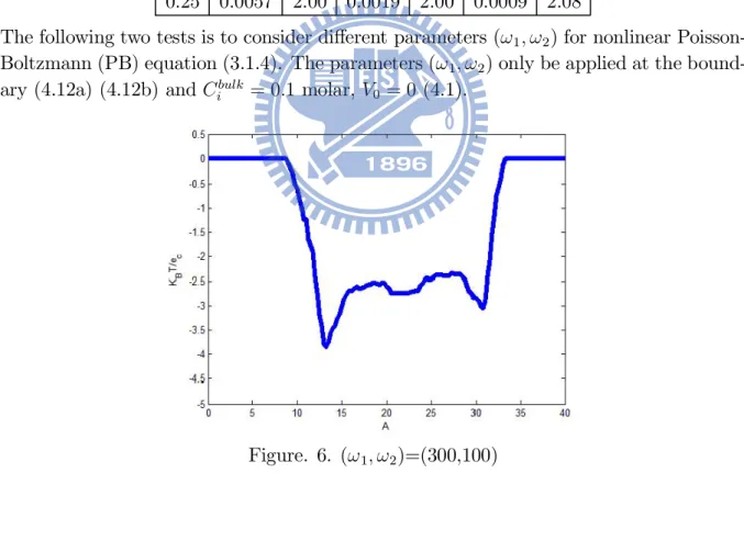
is a function that must be carefully computed. After reading Appendix 2 in [23], we realized that the initial guess function should be set as the solution of the Poisson-Boltzmann (PB) equation ¡r ¢ (()r()) = 4  X =1 (¡ ) + 4 2 X =1 exp(¡()) 2 ­ (3.1.1)

where  _{is bulk concentration of mobile ions of  type are given and other parameter}

are same with (2.1.1). We will need to implement monotone iterative method [17] for both nonlinear PB and PNP models. An electrolyte is any substance containing free ions that make the substance electrically conductive. Electrolyte solutions are normally formed when a salt (NaCl) is placed into a solvent such as water and the individual components dissociate due to the thermodynamic interactions between solvent (water) and solute molecules (NaCl), in a process called solvation. This redistribution of solute molecules in solvent is the focus of Debye-Huckel theory. This theory uses the Boltzmann factor exp(_¡())of dissolved ions with _ in the local electrostatic potential () to estimate the increase or dicrease in the local concetration () relative their bulk concentration



 (), i,e.,

() = () exp(¡()) (3.1.2)

Of course, the potential () is itself in‡uenced by the redistribution of sodium (Na) and chloride (Cl) and by the location of singular charges , so the potentials and

concen-trations must be solved for self-consistently. The bulk concentration 

 () is de…ned

the ratio of the total number of mobile ions of  _{type and the total volume that they}

occupy. It is zero inside the solute and constant outside. The PNP model (2.1.1)-(2.1.3) reduces to the PB model in the absence of a ‡ux, i.e., in the absence of applied voltage, i.e., 0 = 0 in dirichlet boundary condition. The PB equation is usually applied to a 1:1

(negative) of valence ¡. In this case with  = 1, we have 

 () = 0 and 2

X

=1

exp(¡()) = 1exp(¡1())¡ 2exp(¡2())

= 20 exp(_¡1())_{¡ exp(¡2}()) 2 = 20 exp(_¡  ())¡ exp(  ()) 2 = _¡20sinh(  _()) = _¡2 2 0    sinh(   ()) = _¡2  sinh(   ()) (3.1.3) where 2 = ½22_ 0  ,  2 ­ 0,  _{2 ­}

The nonlinear PB equation is thus

¡r ¢ (()r()) + 42  sinh(   ()) = 4  X =1 _(_{¡ })  _{2 ­} (3.1.4) Applying Taylor’s expansion

 = 1 +  1!+ 2 2! + 3 3! +  (3.1.5) to sinh(  ()) with  =  (), we obtain sinh(   ()) =  +  3 6 +  (3.1.6)

The linearized PB equation corresponds to the …rst degree approximation of Taylor’s expansion, i.e., sinh(_

())¼  and is written as ¡r ¢ (()r()) + 42_ = _{¡r ¢ (()r()) + 4}2() = 4  X =1 (¡ )  2 ­ (3.1.7)

Because of delta functions and using the decomposition method previously described, (3.1.1) can be written as ¡r ¢ (()r()) = ¡r ¢ (()re())_{¡ }¢¤¡ ¢0 = 4  X =1 (¡ ) + 4 2 X =1 exp(¡( + e)) (3.1.8)

which yields, in corresponding to (2.2.74), ¡r ¢ (()re()) = 4 2 X =1 exp(¡( + e)) = 4 2 X =1 _  exp(¡e) (3.1.9)  = ½ 0,  2 ­ constant,  2 ­

Similarly, for (3.1.4) and (3.1.7), we have ¡r ¢ (()re()) + 42  sinh(  e()) = 0  2 ­¡ (3.1.10) ¡r ¢ (()re()) + 42e() = 0  2 ­¡ (3.1.11) with 2 = ½22 0  ,  2 ­ 0,  _{2 ­} (3.1.12) The boundary and interface conditions for e are the same as those in (2.2.80) (2.2.86).

3.2

Monotone iterative method for the nonlinear PB equation

Discretization of the left hand side of linear PB equation (3.1.11) by the central …nite di¤erence method (FDM) yields

¡_ Ã (r)e(  )  ! + 42e(  ) ¼ ¡¡12e¡1+ h³ _¡1 2 + + 1 2 ´ + 42_¢2ie ¡ +1₂e+1 ¢2 ,  2 ­n¡ (3.2.1) with 2 = ½220  ,  2 ­ 0,  _{2 ­} (3.2.2)

and for the interface condition, we use the MIB method (2.2.32). Now back to the nonlinear PB equation (3.1.10). Let

 (e) = 42  sinh(  e()),  2 ­n¡ (3.2.3) (e) = _{¡r ¢ (()re}()) + 42  sinh(  e()),  2 ­n¡ (3.2.4) De…ne 0(e) : = lim ¡0 (e + )_{¡ (e})  = lim ¡0 ¡r ¢ (()r(e() + )) +  (e + ) +_{r ¢ (()re}())_{¡  (e})  = lim ¡0 ¡r ¢ (()r()) +  (e + )_{¡  (e})  = _{¡r ¢ (()r) + }0(e) (3.2.5)

Note that the di¤erentiations in ¡r ¢ (()r) and 0_{(e) are di¤erent, i.e., r =}

(___)and 0_{(e) =}  (e)

e etc. The linearized problem of (3.1.10) is thus

0(e(0)) =_{¡r ¢ (()r) + }0(e(0)) = (e(0)),  = e(0) _{¡ e}(1) (3.2.6) then we have

r ¢ (()re1)_{¡ }0(e(0))e(1) =  (e(0))_{¡ }0(e(0))e(0) (3.2.7) [_{¡ }0(e(0))]e(1) =  (e(0))_{¡ }0(e(0))e(0) (3.2.8) where A is a coe¢cient matrix corresponding to the discretization of r ¢ (()re(1)),

0_(e(0)_{) is a diagonal matrix with entries }

 = 0(e (0) ()) with e (0) () =: e (0)  ¼ e(),

e(0) are obtained by linear PB.

The monotone iterative method with FDM for (3.1.10) is to replace (3.2.9) by more general form

[_{¡ ¤]e}(1) =_¡¤e(0)+  (e(0)) (3.2.9) where ¤ can be a constant diagonal matrix or a variable diagonal matrix. Of course if ¤ = 0_(e(0)_{), we have Newton’s method. The MIB method is once again be used on}

4

Dimensionless formulation and approximation of

interface condition

4.1

Unit Conversion and physical constants

For real physical problems, It is important to solve PB and coupled PNP equations in one unit convention. We apply the Gaussian units shown in following tables and the dimensionless process show in next section.

Table 4.1. Physical Constants

Symbol Meaning Value Unit Reference

Å Angstrom 10¡8 _cm

A ampere 1A = 1 C/s A

cal calorie _4.1859£107 _erg

C coulomb 1010/3.336 esu

_K+ di¤usion coe¢cient 2£10¡5 cm2s [24]

_Cl¡ di¤usion coe¢cient 2.03£10¡5 cm2s [24]

 = c elementary (proton) charge 4.8032424£10¡10 esu

 dielectric constant no unit

0 vacuum permittivity 8.8542£10¡12 Cm¡1V¡1

 Planck’s constant _6.6261£10¡34 _{J s}

I current A

J joule 107 _erg

B Boltzmann constant 1.3807£10¡16 erg/K

l liter (volume) cm3

M molar (moles per liter) mol/cm3

mol _6.0221£1023

NA Avagadro’s number 6.0221£1023 mol¡1

 temperature 273.15 + T (C) K

V volt _3.336£10¡3 _erg/esu

Table 4.2.Unit Scale Factors

Name femto pico nano micro milli centi deci kilo mega giga

Pre…x f p n  m c d k M G

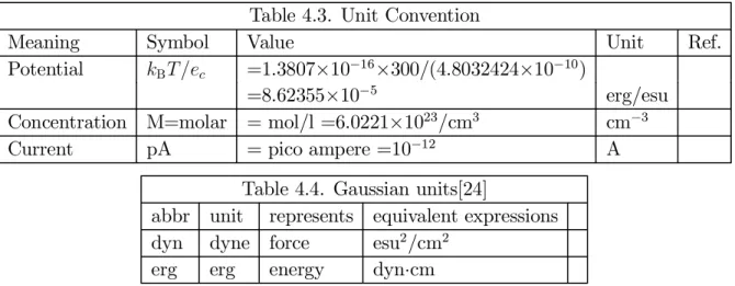
Table 4.3. Unit Convention

Meaning Symbol Value Unit Ref.

Potential B  =1.3807£10¡16£300/(4.8032424£10¡10)

=8.62355£10¡5 _erg/esu

Concentration M=molar _{= mol/l =6.0221£10}23_/cm3 _cm¡3

Current pA = pico ampere =10¡12 _A

Table 4.4. Gaussian units[24]

abbr unit represents equivalent expressions dyn dyne force esu2_/cm2

erg erg energy _dyn¢cm

4.2

Dimensionless formulation

Physical phenomena within a channel system are controlled by boundary conditions (BCs). We now describe the BCs of the PNP system. For the Poisson equation (2.1.1), the voltage applied to the system is given by the potential di¤erence (a Dirichlet BC), denoted by 0  0 and shown in Fig. 4, along the  direction, and a Neumann BC on

other parts of ­, namely,

¡  0Å¢ = 0, 

¡

  40Å¢= 0 (4.1)



n = 0, for jj = 20 or jj = 20 and  6= 40 and 0 (4.1(a))

The unit of 0 is mV (milli volt). The boundary data for  is similarly denoted by 0

in the unit of M (molar). Moreover, a single value of 0 is assumed for both 1(  )

and 2(  )on ­ \ ­, i.e.,

₁(  ) = ₂(  ) = _{0, 8 (  ) 2 ­ \ ­}. (4.2) For this project, the dielectric constants are set to

 = 2 = 80 (4.3)

and the di¤usion coe¢cients in bulk are given in Table 4.1. Note that the Gaussian units are adopted in [24]. The fundamental di¤erence between the SI (International System of Units) and Gaussian units lies in the presentation of Coulomb’s law

 = 12

402

[SI] = 12

where CGS stands for centimetre-gram-second. Note that the vacuum permittivity 0

does not appear in the Gaussian format (in [24]).

Let  = 1Å(10¡8_{). By using the following scalings with the new dimensionless}

quantities marked by the subscript (or supscript)

 =    =    =   (4.5) e = e  B , _ =   , _ =  2_2  B , _=  2 (4.6)

Eq. (2.2.74) can be written as ¡r¢ µ _B 2_  r e ¶ = 2 P =1  ¡r¢ ³ re ´ = 2 P =1  _ 2_2  _B = 2 P =1 __ (4.7) where r= D       E

. And (2.1.2) and (2.1.3) can be expressed as 1 2r¢  · r+ B   B r ¸ = 0 1 2r¢ [r+   r] = 0 B 2_2  r¢ [r+     r] = 0 r¢ [r+     r] = 0 (4.8)

We further check the unit of   that _ =  2_2  _B = 60221_{£ 10}23 £ 10¡16_{£ (48032424)}2 £ 10¡20 13806620_{£ 10}¡16_{£ 300} = 3354257 · cm2_esu2 cm3_{¢ erg} = esu2

esu2 (no unit)

¸  (4.9(a)) e = e  B = 48032424£ 10 ¡10 300_{£ 13806620 £ 10}¡16 " V esu erg = J Cesu erg = J esu C erg = 107_{erg esu} 101 0 3.336esu erg # = 48032424£ 10 ¡10 300_{£ 13806620 £ 10}¡16 ¢ 107 1010 3336 · erg esu

esu erg(no unit) ¸

Moreover, we verify a similar unit de…ned in [24] using its notation (see Eq. (52) in [24] where 1 dyne = esu2_{cm should be 1 dyne = esu}2_{cm in Table 5)}

B c = 1380662£ 10 ¡16_{£ 300} 48032424_{£ 10}¡10 · dyn cm esu = esu2 esu = esu cm ¸ (4.10) = 08623_{£ 10}¡4 hesu cm i 1 [dyn] = 1hg cm s2 i = 10¡5 [N] , 1 [esu] = 1hdyn12cmi 1 [_{erg] = 1 [dyn ¢ cm] = 10}¡7 [J]  J = kg ¢ m 2 s2 =N ¢ m 1 [_{esu] = 3336 £ 10}¡10 [C] (4.11)  = e©  300_{£ }B = e© 1 300_{¢ 08623 £ 10}¡4 = 386563e© (4.12a) 200mV  300B = 002580 [ no unit ( by (4.9(b)) )] e  =  NA22c 103_ B =  60221_{£ 10}23 £ 10¡16 _{£ (48032424 £ 10}¡10₎ 103 _{£ 08623 £ 10}¡4

= 033545 [no unit ( by (4.9(a)) )] (4.12b)

e   = 00008677 e ©

From above relations, we observe that the Gaussian units are quite complicated and that the scaled concentration (4.7) and (4.8) is dimensionless. We will use the CGS-Gaussian units.

Remark 4.1. The above scaling convention is used in our code. For example, the coordinate system of the domain is expressed by (4.5) and the dielectric constants are exactly given as (4.3). Consequently, the BC (4.1) is also required to be scaled as

₀ = 0  B = 386858_£ 1 103 = 00386858 · V V (no unit) ¸ . (4.13) We thus have 0 = 100mV =) 0= 386858 (4.14)

Similarly, for (4.2), we have by ( 4.9(a) )

0 = 1M (molar) =) 0= 3354257 (4.15)

Note that we can scale Eq. (4.8) further as (4.8)

100 =)



0

Moreover, we also have _K+ = 1, _Cl¡ =¡1, (4.17)  K+ = 2_{£ 10}¡5 10¡16 · cm2 cm2 _s ¸ = 2_{£ 10}11 · 1 s ¸ _Cl¡ = 2_{£ 10}¡5 10¡16 · cm2 cm2 _s ¸ = 203_{£ 10}11 · 1 s ¸ (4.8) 1011 =)  K+ 1011 = 2,  Cl¡ 1011 = 203

Remark 4.2. Following [24], the di¤usion coe¢cient pro…les are de…ned via an interpo-lation function along the -axis (the channel axis)

 (r) =  () =  µ _{¡ ch} bu¡ ch ¶+1 ¡ ( + 1) µ _{¡ ch} bu ¡ ch ¶ (4.18) where  ¸ 2 is an integer,  2 [ch bu] which is a bu¤ering region between the channel

pore and bulk regions. The di¤usion coe¢cient function is then de…ned by

(r) = 8 < : ch r2 Channel region ch+ (ch¡ bu) (r) r2 Bu¤ering region _bu r_{2 Bulk region} (4.19) bu = K+ or bu = Cl¡ and ch = 005bu (4.20)

The bu¤ering region is set (symmetrically about  = 0) to

bu¡ ch = 55 9Å , bu = 13Å, if  = 2 bu¡ ch = 35 9Å , bu = 13Å, if  = 9 bu¡ ch = 20 9Å , bu = 13Å, if  = 19 (4.21) Example 4.1. Nonlinear GA PNP, Singualr Charges, Di¤usion Function (4.19), no Exact Solutions. We now try to reproduce the results of Figure 9 and Table 6 in [24]. The BC data for this case are as follows:

0 = 200mV, 0 = 01M =) 0 = 773716, 0 = 3354257 (4.22)

The …rst thing needed attention is scaling. From above dimensionless analysis, the orders of (4.14) and (4.15) are (1) and (102_{), respectively. The code will blow up if (4.16) is}

not used. Therefore, the scaled variables e and 

 in (4.6) should be changed to e = e    ,    =  2_2    ,   0 = 773716  ,   0 = 3354257  (4.23)

where the scaling factors 1 and 2 are crucial for the convergence behavior of Gummel’s

algorithm and will be chosen from the coding experience. Accordingly, (2.2.79) should be scaled as follows ¡r ¢ (r) = ¡r ¢ ³ r(e + ) ´ (4.24) = _¡ µ 1B 2_ ¶ h r¢ ³ re ´ + ¢¤+ ¢0 i = 4  P =1 (r¡ r) + 4 2 P =1  ¡hr¢ ³ re ´ + ¢¤+ ¢0 i = µ 2_  1B ¶ " 4  P =1 (r¡ r) + 4 2 P =1  # = 4  P =1   (r_{¡ r}) 2_2  1B + 4 2 P =1    2_2  1B = 4  P =1 _(r¡r) + 4 2 1 2 P =1 __, (4.25a) ¡hr¢ ³ re ´i = 42 1 2 P =1 __, 3 = 2 1 (4.25) Therefore, (r¡r) = (r¡ r) 2_2  1B , ¤_ = ¤  1B , 0_ = 0  1B (4.26) By (2.2.77), we also have ¤_(r) = 2  1B  P =1 __ _p(_{¡ })2_{+ (} ¡ )2+ (¡ )2 = 1  P =1 _  p (¡ ) 2_{+ (} ¡ ) 2_{+ (} ¡ ) 2, 1 = 2_ 1B  (4.27) 1 = 2  1B  = 48032424£ 10 ¡10 1£ 08623 £ 10¡4£ 10¡8 · esu2 erg £ cm ¸ = 5570268 1 [no unit] (4.28)

Now we consider NP equations r ¢ () · r() + _ B ()_re() ¸ = 0 1 2r¢ () · r() + 1B   B ()_re  () ¸ = 0 r¢ () h r() + 1()re  ()i = 0 2B 2_2  r¢ () h r() + 1()re  ()i = 0, r¢  h r+ 1re i = 0, 2 = 1 (4.29)

The linear PB equation(3.1.7) given by

¡r ¢ (()r()) + 42() = 4  X =1 _(_{¡ })  _{2 ­} by (4.5) and (4.23), we obtain ¡_ 1 2 r ¢ (r()) + 4  _ 22  _ 1() = _¡ 1 2 r ¢ (r()) + 8  2_2  ₂₁_(_) =  1 2 [_¡r¢ (r()) + 82()] Therefore [_¡r¢ (r()) + 82()] =  2  1 4  X =1 (¡ ) = 4  X =1 _(¡ ) (4.30)

Scaling nonlinear PB equation ( 3.1.4)

¡r ¢ (()r()) + 42_  sinh(   ()) = 4  X =1 (¡ ) 2 ­

we have ¡r ¢ (()r()) + 42_  sinh(   ()) =  1 2 [_¡r¢ (r()) + 8 2 1 _sinh(1())] Therefore [_¡r¢ (r()) + 8 2 1 _sinh(1())] = 4  X =1 _(¡ ) (4.31)

4.3

Approximation of interface conditions

Due to the interface condition (2.2.86) and 0 is only de…ned in ­, we remark that

the following extrapolation scheme is also described in Section D in [11]. We now de-rive a nonlinear extrapolation formula for this case from which we can approximate the derivative   0_( +1₂) =   0_( ).

Case I. {_¡2, _¡1, g ½ ­, +1₂ 2 ¡, +1, +22 ­ (see Fig. 5.).

0() = 0+ 1 + 22+ 33+ 44 (4.32)   0_( ) ¼ 1+ 22 + 332 + 443 _¡1 = 0+ 1¡1+ 22_¡1 + 33_¡1+ 44_¡1 _ = 0+ 1+ 22 + 33 + 44 _ = ₀+ ₁_ + ₂2  + 33 + 44 _+1 = 0+ 1+1+ 22+1 + 33+1+ 44+1 _+2 = 0+ 1+2+ 22+2 + 33+2+ 44+2

where the values of _+1and _+2 are obtained by the following two extrapolation formulas similar to (4.32) 0() = 0+ 1 + 22+ 33 _¡2 = 0+ 1¡2+ 22_¡2+ 33_¡2 _¡1 = 0+ 1¡1+ 22_¡1+ 33_¡1 _ = 0+ 1+ 22 + 33 _ = 0+ 1 + 22 + 33+ 44 _+1 = 0(+1) (4.33)