線性橢圓偏微分方程

國立交通大學

應用數學系

碩士論文

線性橢圓偏微分方程

Topics on Linear Elliptic Equations

研究生 : 姚文雯

指導教授 : 李榮耀 博士

線性橢圓偏微分方程

Topics on Linear Elliptic Equations

研 究 生 : 姚文雯 Student : Wen-Wen Yao

指導教授 : 李榮耀 博士 Advisor : Dr.Jong-Eao Lee

國立交通大學

應用數學系

碩士論文

A Thesis

Submitted to Department of Applied Mathematics

College of Science

National Chiao Tung University

In Partial Fulfillment of the Requirements

for the Degree of Master

in

Applied Mathematics

June 2007

Hsinchu，Taiwan，Republic of China

線性橢圓偏微分方程

學生：姚文雯 指導教授：李榮耀 博士

國立交通大學應用數學系

摘 要

研究線性橢圓偏微分方程(線性橢圓 PDEs) 。首先, 給一些實用的例

子, 同時將二階線性偏微分方程式作一分類。接下來, 運用幾個古典方

法解線性橢圓偏微分方程,並且將該方程式的解以各種形式表示。

當我們運用傅立葉轉換解整個或半平面的偏微分方程時, 需要利用

逆傅立葉轉換導出該偏微分方程的解, 此時被積分函數中常出現平方根

的形式, 在複數平面上它是多值函數。為了讓逆傅立葉轉換導出的解是

正確的, 我們結合複數平面上的黎曼曲面,藉由適當的代數建構出平方

根在該曲面上是單值, 並且完成逆轉換的解析解與數值解。最後藉由例

子來說明整個計劃。

Topics on Linear Elliptic Equations

Student : Wen-Wen Yao Advisor : Dr.Jong-Eao Lee

Department of Applied Mathematics, National Chiao Tung University

Abstract

We study the linear elliptic partial differential equations ( linear elliptic PDEs ). First, we give some practical examples and show that they are governed by such type of the equations. Next, we apply several classical methods to solve the linear elliptic PDEs with the solutions being expressed in various forms. We then identify those solutions.

When we apply Fourier transformations to the whole- and half-line PDEs, it is necessary to perform the inverse Fourier transformations to derive the PDE solutions, and it is quite often that those integrals involve the square root operator which is multi-valued in the complex plane. In order to perform the inverse transformations correctly, we develop the Riemann surfaces from the complex plane with the proper algebraic structures to assure that the square root is now a single-valued function on the surfaces, and we are able to accomplish the inverse transformations analytically and numerically. Some examples are given to illustrate the entire scheme.

誌

誌

誌

誌 謝

謝

謝

謝

在交通大學兩年的研究所生涯中，承蒙恩師 李榮耀教授在論文研究

上的悉心指導與建議，始能順利完 成，在此向恩師致上最誠摯的感謝。

論文撰寫過程中特別感謝佳樺、美如所給予的鼎力協助。感謝父母

親的養育與栽培、老公的鼓勵及家人的配合，你們所給予的支持是我完

成論文最大的原動力。一 路 行 來，點 滴 在 心，雖 然 這 不 是 一 部 完 美

的 論 文 ， 但 這 部 論 文 的 完 成 ， 要 感 謝 的 真 的 人 很 多 ， 無 法 一 一

列 出 ， 僅 以 此 文 表 達 我 的 誠 摯 謝 意 。

Contents

Ⅰ. Introduction--- 1

Ⅱ. The methods of solving Elliptic PDE ---14

Ⅱ-1 Separation of variableto construct solution of Laplac ′es equation---14

Ⅱ-1.1 The domain is rectangular ---14

Ⅱ-1.2 The domain is circular ---20

Ⅱ-2 Finite Fourier transform to construct solution of Laplac ′es equation---23

Ⅱ-3 Fourier transform to construct solution of Laplac ′esequation---28

Ⅱ-4 Finite difference to construct solution of Laplac ′es equation---32

Ⅲ. The limit of the methods of solving Elliptic PDE ---36

Ⅳ. Integral evaluations on two-sheeted Riemann surface of genus N ---39

Ⅳ-1 Fundamental introduction---39

Ⅳ-2 Riemann surface of the algebraic curve

∏

= − = n j j z z z f 1 ) ( ) ( with z_j∈ ---- 42 R Ⅳ-2.1 The horizontal cut structure of f(z)---42

Ⅳ-2.2 The algebraic and geometric structure for Riemann surface of f(z)--46

Ⅳ-3 Riemann surface of the algebraic curve

∏

= − = n j j z z z f 1 ) ( ) ( with z_j∈C-50 Ⅳ-3.1 The vertical cut structure of f(z)---51

Ⅳ-3.2 The algebraic and geometric structure for Riemann surface of f(z)----53

Ⅳ-4 The integrals over canonicala, cycles for horizontal cuts and vertical cuts---56 b Ⅳ-4.1 The a, cycles over the Riemann surface of b

∏

= − = n j j z z z f 1 ) ( ) ( ---56

Ⅳ-4.2 About〝Mathematica〞and How to modify ---59

Ⅳ-4.3 An application for the integrals over a, cycles---60 b Ⅳ-5 An application for Riemann integrals---65

Ⅰ

Ⅰ

Ⅰ

Ⅰ. . . .

Introduction

Many important scientific and engineering problems fall into the field of second-order partial differential equation. We want to recognize the distinguish for second-order partial differential equation.

The distinction as to Hyperbolic 、 Parabolic 、or Elliptic for second-order partial differential equation depends on the coefficients of second-derivative term. we can write any such general linear partial differential equation of second order in two variables reads，

0 ) , ( ) , ( ) , ( ) , ( ) , ( ) , (x y u +B x y u +C x y u +D x y u +E x y u +F x y u= A _{xx xy yy x y} where (x,y)∈Ω (Ω is domain ).

Depending on the value B2−4AC，we classify the equation as

Hyperbolic ⇒ if B2−4AC ＞ 0 ,

Parabolic ⇒ if B2−4AC ＝ 0 ,

Elliptic ⇒ if B2₋4AC _{＜ 0 .}

For example，the Wave equation u_xx−u_yy =0 is of Hyperbolic type，and the

Heat partial differential equation uxx−ut =0 is parabolic，while Laplac ′ equation es 0

= + _yy

xx u

u is Elliptic .

Elliptic partial differential equation has many applications in engineering，physics and material science，for example resistance and capacitance extraction in electronic circuit， state decomposition in microwave tube，Navier-Stokes equation in incompressible fluid and device simulation of semiconductor，membrane displacement，torsion and so on .

There is a question，why are most physical problems related to elliptic equation？ Since Elliptic equation has a term 〝 Laplacian operator 〞， it describe diffusion

phenomenon，like heat diffusion、dynamic diffusion etc.

Now consider the steady potential flow in two-dimensional incompressible fluid. First，we define correlation proper noun. In general，the two-dimensional flow is a flow in which the velocity component depends on only two space variables. An example is a plane

flow，in which the velocity component depends on two spatial coordinates，x and y ， but not z . An incompressible flow exists if the density of each fluid particle remains relatively constant as it moves through the flow field，that is =0

dt dρ

，and for an

incompressible flow ， the differential equation of mass conservation is

0 = ∂ ∂ + ∂ ∂ + ∂ ∂ z u y u x

ux y _{z in three-dimensional. The velocity at a given point in space does}

not vary with time，that is =0 ∂ ∂

t u

.We call that is the steady flow. The flow is irrotational we call the potential flow. In this we discuss xy− plane，that implies wz =0，we have

y u x u_{y x} ∂ ∂ = ∂ ∂ .

Let u(x,y)be the velocity of the point (x,y) on xy− plane. Then we have the differential of mass conservation of incompressible flow in xy− plane.

=0 ∂ ∂ + ∂ ∂ y u x ux y _{. ( 1-1 )}

This equation is satisfied identically if a function ψ(x,y)is defined such that becomes ( ) ( )=0 ∂ ∂ − ∂ ∂ + ∂ ∂ ∂ ∂ x y y x ψ ψ . ( 1-2 ) Comparison of (1-1) and (1-2) shows that this new function ψ must be defined such that

y u_x ∂ ∂ = ψ and x u_y ∂ ∂ − = ψ . ( 1-3 ) Since this flow is irrotational，we put (1-3)into the

y u x u_{y x} ∂ ∂ = ∂ ∂ . We get ₂ 2 2 2 y x ∂ ∂ = ∂ ∂ − ψ ψ ⇒ ₂ 0 2 2 2 = ∂ ∂ + ∂ ∂ y x ψ ψ ⇒ ( ₂) 2 0 2 2 2 = ∇ = ∂ ∂ + ∂ ∂ ψ ψ y x . ( 1-4 ) The operator 2 ( _{2 2}) y x ∂ ∂ + ∂ ∂ =

∇ is called the Laplacian ，and the equation (1-4) is

calledLaplac ′es equation in two dimensional. The inviscid、incompressible、irrotational flow fields are governed by Laplac ′ equation. This type of flow is commonly called es

In below，we illustrate the angular motion in thexy− plane. The velocity variation that causes rotation and angular deformation is illustrated in Figure 1-1(a). In a short time interval ∆ the line segments OA and OB will rotate through the angles t δα and δβ

to the new positions O ′ and A O ′ as is shown in Figure 1-1(b). B

(a) (b)

Figure1-1. Angular motion and deformation of a fluid element

The angular velocity of line OA ，W_OA is

t W t OA ∆ = → ∆ δα 0 lim .

For small angles，we have

t x u x t x x u x A A y y ∆ ∂ ∂ = ∆ ∆ ∆ ∂ ∂ = ∆ ′ = ≈ δα δα tan . So that x u t t x u W y u t OA ∂ ∂ = ∆ ∆ ∂ ∂ = → ∆lim0[ ] . Note that， if x u_y ∂ ∂

is positive，W_OA will be counterclockwise. Similarly，the angular velocity of line OB ，W_OB is

t W t OB ∆ = → ∆ δβ 0 lim , and t y u y t y y u y B B _x x ∆ ∂ ∂ = ∆ ∆ ∆ ∂ ∂ = ∆ ′ = ≈ δβ δβ tan , so that y u t t y u W x x t OB ∂ ∂ = ∆ ∆ ∂ ∂ = → ∆lim0[ ] .

Note that ，if

y u_x

∂ ∂

is positive，W_OB will be clockwise.

A’ O A B B A O B’ x x u uy y ∆ ∂ ∂ + y y u u x x ∆ ∂ ∂ + x u y u x ∆ y ∆ y ∆ x ∆ t y y ux _{∆ ∆} ∂ ∂ t y y ux _{∆ ∆} ∂ ∂ δβ δα

The rotation，W ，of the element about the _Z Z −axis is defined as the average of the abgular velocities W_OA and W_OB of the two mutually perpendicular lines OA and OB . Thus，if counterclockwise rotation is considered to be positive，it follows that

) ( 2 1 y u x u W y x Z ∂ ∂ − ∂ ∂ = .

Since we derive in xy− plane，that implies WZ =0 . So we get y u x u x y ∂ ∂ = ∂ ∂ .

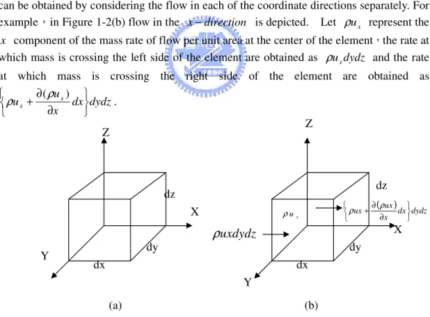
We will take as our control volume the small，stationary cubical element shown in Figure 1-2(a). At the center of the element the fluid density is ρ and the velocity has component u 、_x u_y and u . The rate of mass flow through the surface of the element _z

can be obtained by considering the flow in each of the coordinate directions separately. For example，in Figure 1-2(b) flow in the x−direction is depicted. Let ρu_x represent the

x component of the mass rate of flow per unit area at the center of the element，the rate at which mass is crossing the left side of the element are obtained as ρu_xdydz and the rate at which mass is crossing the right side of the element are obtained as

dydz dx x u u_x x       ∂ ∂ + (ρ ) ρ . (a) (b)

Figure 1-2. A differential element for the development of conservation of mass

When these two expressions are combined，the net rate of mass flowing from the element through the two surfaces can be expressed as ﹕

dy X Y Y dz X dx dz dy dx

uxdydz

ρ

( )_{dx dydz} x ux ux       ∂ ∂ + ρ ρ x u ρ Z Z

Net rate of mass outflow in x−direction = dx dydz x u u_x x       ∂ ∂ + (ρ ) ρ － ρu_xdydz = dxdydz x ux ∂ ∂(ρ ) .

For simplicity，only flow in the x−directionhas been considered in Figure 1-2(b)， in general，there will also be flow in the y and z−direction. An analysis similar to the one used for flow in the x−direction shown that

Net rate of mass outflow in y−direction = dy dxdz

y u u_y y       ∂ ∂ + (

ρ

)

ρ

－ ρu_ydxdz = dxdydz y u_y ∂ ∂(ρ ) , and

Net rate of mass outflow in z−direction = dz dxdy

z u u z z       ∂ ∂ + (ρ ) ρ － ρu_zdxdy = dxdydz z u_z ∂ ∂(ρ ) .

Since we derive the incompressible flow， i.e. =0 ∂ ∂

t

ρ

and ρ is constant. Thus by the conservation of mass，we have

Net rate of mass outflow = ( ) ( ) ( ) =0

∂ ∂ + ∂ ∂ + ∂ ∂ dxdydz z u dxdydz y u dxdydz x ux ρ y ρ _z ρ ⇒ ( ) ( ) ( ) =0 ∂ ∂ + ∂ ∂ + ∂ ∂ z u y u x ux ρ y ρ _z ρ . Since ρ is constant. Therefore =0 ∂ ∂ + ∂ ∂ + ∂ ∂ z u y u x u_x y _z .

As previously mentioned，this equation is also commonly referred to as the continuity equation.

In below，we consider the a situation that is typical，in which the temperatures is a function of the coordinates of position of the point in equation.

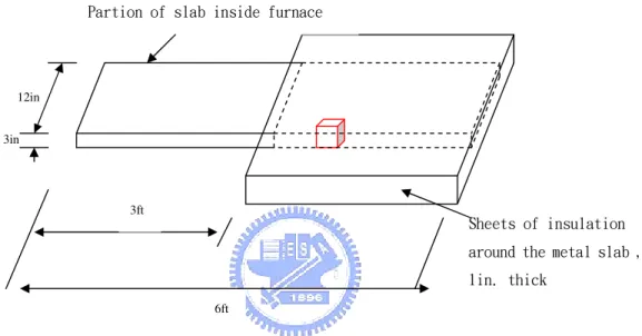
A piece of metal is 12in.× 3in.× 6ft. There feet of the slab is kept inside a furnace but half of the slab protrudes (see Figure 1-3 ). In order to decrease heat losses to the air，the protruding half is covered with a 1-in.thickness of insulation. If the furnace is maintained at 9500F，will at points of the metal reach a temperature of 8000For higher，in spite of heat loss through the insulation？ Such a question might arise in heat-treating the slab when the only furnace available to heat the metal is too small to contain the whole slab.

Figure 1-3. A piece of metal is 12in.× 3in.× 6ft

We derive the relationship for temperature u as a function of space variables for the equilibrium temperature distribution by the metal piece protruding from the furnace. In this consider the two spatial coordinates，that is derive the relationship for temperature u as a function of space variables xand y for the equilibrium temperature distribution on a flat plate.

First，ideal supposition. One：consider only the case where the temperatures do not change with time. Second：assume that heat flows only in the x and y -directions and not in the perpendicular direction ( If the plate is very thin，or if the upper and lower surfaces are both well insulated，the physical situation will agree with our assumption ) . Three：assume that no heat is being generated at points in the plate. ( see Figure 1-4 )

12in 3in

6ft 3ft

Partion of slab inside furnace

Sheets of insulation around the metal slab , 1in. thick

Figure 1-4. The plate which is thin and small

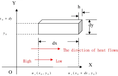
Let h be the thickness of the plate. Heat flows at a rate proportional to the cross-sectional area，to the temperature rate of change (u_xor u_y)，and to the thermal conductivity k ，which we will assume constant at all points. The flow of heat is from high to low temperature，of course，meaning opposite to the direction of increasing temperature rate of change. We use a minus sign in the equation to account for this：

In the x-directions ，the rate of heat flow into element at x= x₀ is -k(hdy)u_x . The rate of change at x0+dx is the rate of change at x0 plus the increment in the rate of

change over the distance dx ：

The rate of change at x0+dx： ux+uxxdx .

Rate of heat flow out of element at x= x0+dx： -khdy[ux +uxxdx] .

Net rate of heat into element in x-directions ﹕ -k(hdy)[u_x−(u_x+u_xxdx)]=kh(dxdy)u_xx . Similarly，in the y -directions we have the Net rate of heat into element in y -directions ：

-khdx[u_y −(u_y+u_yydy)]=kh(dxdy)u_yy .

The total heat flowing into the elemental by conduction is the sum of these net flows in the x and y -directions. If there is equilibrium as to temperature

distribution，that is steady-state，the total rate of heat flow into the element plus heat generated must be zero.

dy y0 + 0 y O X Y dx dy h

The direction of heat flows Low High ) , (x0 dx y0 ux + ) , (x0 y0 ux

Hence 0 ) ( ) )( (dxdy u +u +Qhdxdy = kh _{xx yy}

where Q is the rate of heat generation per unit area and Q will often be a function of

xand y .

By above assume second，we have Q=0 ，

and 0 ) )( (dxdy uxx+uyy = kh ⇒ _{u +u =∇}2_{u =}0 yy xx . ( 1-5 ) The operator 2 ( _{2 2}) y x ∂ ∂ + ∂ ∂ =

∇ is called the Laplacian ，and the equation (1-5) is

calledLaplac ′ equation in two dimensional. es Laplac ′ equation arises in es

steady-state heat conduction problems involving homogeneous solids. For three dimensional heat flow problems，we would have，analogously，

0 ) ( _{2 2 2} 2 ₌ ∂ ∂ + ∂ ∂ + ∂ ∂ = ∇ u z y x u .

Consider that heat is being generated at points in the plate. Assume this removal rate to be a function of the location of the element in the xy− plane， f(x,y)，we would have，with Q equal to the rate of heat generation per unit area，

0 ) ( ) , ( ) )( (dxdy u +u +Q x y h dxdy = kh _{xx yy} ⇒ kh(dxdy)(∇2u)=−Q(x,y)h(dxdy) ⇒ k(∇2u)=−Q(x,y) ⇒ 2 1Q(x,y) f(x,y) k u =− = ∇ .

This equation is called Poisso ′ equation ( non homogeneous ). ns

A typical steady-state heat flow problem is the following： A thin steel plate is a 20

10× an rectangular. If one of the 10-cm edges in held at 1000C and the other three edge are held at 00C，what are the steady-state temperatures at interior points？ For steel，k =0.16cal /sec•cm • C2 0 / cm .

Math model：Find u(x,y) such that 0 2 2 2 2 = ∂ ∂ + ∂ ∂ y u x u , 100 ) 0 , (x = u ， 0 ) 20 , (x = u ， 0 ) , 0 ( y = u ， 0 ) , 10 ( y = u .

In this statement of the problem，we imagine one corner of the plate at the origin，with boundary conditions as sketched in Figure 1-5.

Figure 1-5. Laplac ′ equation for a rectangular domain es

Because the field of application of Laplac ′ equation and es Poisso ′ equation do ns

not involve time，initial conditions are not prescribed for the solution of equation. Rather，we find that it is proper to simply prescribed a single boundary condition. Such problems are them call simply boundary value problems ( BVPs ).

The basic example of an elliptic partial differential equation is Laplac ′ equation，es

0 .

._{e∇ u}2 ₌

i in Ω ( that is domain ) in n−dimensional Euclidean space，other examples of elliptic partial differential equations include the nonhomogeneousPoisso ′ns equation，

) , ( . . 2 y x f u e

i ∇ = in Ω ( that is domain ). These two equations include most of the physical applications of elliptic partial differential equation.

Elliptic partial differential equation may have non-constant coefficients and be non-linear. Despite this variety，the elliptic equations have a well-developed theory. In this paper，we discuss the linear Elliptic partial differential equation.

O Y X 0 = u u=0 0 = u 0 = u 0 = + _yy xx u u

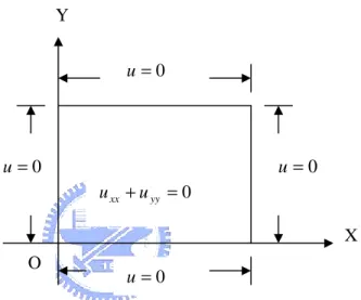
By above math model，we know in two dimensions，Laplac ′ equation has the es

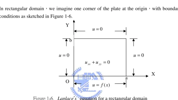
rectangular coordinate representation： ₂ 0 2 2 2 = ∂ ∂ + ∂ ∂ y u x u for 0＜ x ＜ a and 0＜ y ＜ b , u(x,0)= f(x) , 0 ) , (x b = u , 0 ) , (o y = u , 0 ) , (a y = u .

In rectangular domain，we imagine one corner of the plate at the origin，with boundary conditions as sketched in Figure 1-6.

Figure 1-6. Laplac ′ equation for a rectangular domain es

Many two dimensional problems involving Laplac ′ equation are in region that es

lend themselves to a polar description in terms of r and θ，rather than rectangular coordinates x and y . This means that we need an expression for the Laplacian in terms of polar coordinates.

Let us consider in the unit circle x2 +y2＜1 with its values given on the boundary 1

2 2

= + y

x . It is natural to introduce the poor coordinates transformation.

(x,y) → (r,θ) _{r= x}2 _+y2 Y O Y X 0 = u u =0 0 = u ) (x f u= 0 = + yy xx u u a b y x O Θ X

Setting    = = θ θ sin cos r y r x and x y = θ

tan ⇒ =tan−1 =tan−1(yx−1)

x y

θ

We want to (x,y)−PDE ⇒ (r,θ)−PDE

) ( ) ( ) ( ) ( 1 ) 2 ( ) ( 2 1 2 2 2 1 2 2 2 2 2 1 2 2 y x y u x y x u x y yx u x y x u u r u u_{x r x x r r} + − ⋅ + + ⋅ = + − ⋅ + + ⋅ = ⋅ + ⋅ = − − − θ θ θ θ ] ) ( ) )( 2 ( ) ( 2 1 [ ) ( ) ]( [ 2 1 2 2 2 3 2 2 2 1 2 2 ₊ − ₊ − ₊ − _{+ +} − ⋅ + ⋅ = u r u x y x u x y x x x y u_{xx rr x r}θ θ_{x r} )] 2 ( ) )( 1 )( [( ) ]( [ _{2 2} u y x2 y2 2 x y x y r u u _{x r x} + − − + − + − ⋅ + ⋅ + θθ θ θ θ ] ) ( ) )( [( ) ( ) )]( ( ) ( ) ( [ 2 1 2 2 2 3 2 2 2 2 1 2 2 2 2 2 1 2 2 − ₊ − _{+ − +} − _{+ +} − + − ⋅ + + ⋅ = x y x u x x y x y y x y u x y x u_{rr rθ r} [ ( ) ( ) ( )]( ) [(2 )( 2 2) 2] 2 2 2 1 2 2 2 2 − − + + + − + ⋅ + + − ⋅ + u xy x y y x y x y x u y x y uθθ θ_r θ ) ( ) ( ) ( ) ( 1 ) 2 ( ) ( 2 1 2 2 2 1 2 2 2 1 2 1 2 2 y x x u y y x u x y x u y y x u u r u u_{y r y y r r} + ⋅ + + ⋅ = + ⋅ + + ⋅ = ⋅ + ⋅ = − − − θ θ θ θ ] ) ( ) )( 2 ( ) ( 2 1 [ ) ( ) ]( [ 2 1 2 2 2 3 2 2 2 1 2 2 ₊ − ₊ − ₊ − _{+ +} − ⋅ + ⋅ = u r u x y y u x y y y x y u_{yy rr y r}θ θ_{y r} ] ) )( 2 [( ) ]( [ _{2 2} + − 2 + 2 −2 + ⋅ + ⋅ + u xy x y y x x r u u_θθ θ_{y θr y θ} ] ) ( ) )( [( ) ( ) )]( ( ) ( ) ( [ 2 1 2 2 2 3 2 2 2 2 1 2 2 2 2 2 1 2 2 − ₊ − _{+ − +} − _{+ +} − + ⋅ + + ⋅ = x y y u y x y x y y x x u y y x u_{rr rθ r} [ ( ) ( ) 2( )]( _{2 2}) [( 2 )( 2 2) 2] 1 2 2 2 2 − − + − + + + ⋅ + + ⋅ + u xy x y y x x y y x u y x x uθθ θ_r θ

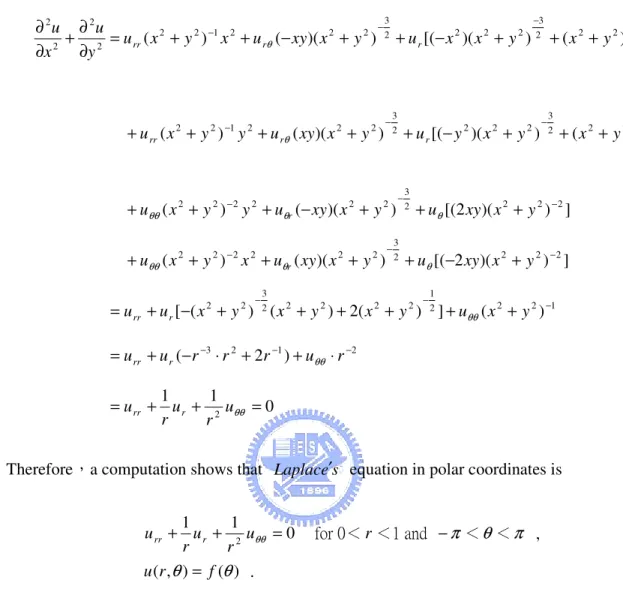
Hence ] ) ( ) )( [( ) )( ( ) ( 2 1 2 2 2 3 2 2 2 2 3 2 2 2 1 2 2 2 2 2 2 − ₋ − − _{+ − + + − + + +} + = ∂ ∂ + ∂ ∂ y x y x x u y x xy u x y x u y u x u r r rr θ ] ) ( ) )( [( ) )( ( ) ( 2 1 2 2 2 3 2 2 2 2 3 2 2 2 1 2 2 ₊ − _{+ +} − _{+ − +} − _{+ +} − +u_rr x y y u_rθ xy x y u_r y x y x y ( ) ( )( ) 2 [(2 )( 2 2) 2] 3 2 2 2 2 2 2₊ − _{+ − +} − _{+ +} − +u_θθ x y y u_θr xy x y u_θ xy x y ( ) ( )( ) 2 [( 2 )( 2 2) 2] 3 2 2 2 2 2 2₊ − _{+ +} − _{+ − +} − +uθθ x y x uθ_r xy x y uθ xy x y ₂ 2 2 1 1 2 2 2 2 2 3 2 2 ) ( ] ) ( 2 ) ( ) ( [− + − + + + − + + − + =u_rr u_r x y x y x y u_θθ x y 3 2 1 2 ) 2 (− − ⋅ + − + ⋅ − + =u_rr u_r r r r u_θθ r = +1 + 1₂ uθθ =0 r u r u_{rr r}

Therefore，a computation shows that Laplac ′ equation in polar coordinates is es

+1 + 1₂ uθθ =0 r u r u_{rr r} for 0＜ r ＜1 and − ＜π θ＜π , u(r,θ)= f(θ) .

In circular domain，with boundary conditions as sketched in Figure 1-7.

Figure 1-7. Laplac ′ es equation for a circular domain ) (x f u= Θ 1 Y X

0

2

=

∇ u

Laplac ′ equation，also called the potential equation，the concept of a potential es

function seems to have been first used by Daniel Bernoulli ( 1700 ~ 1782 )，son of the more famous Jean Bernoulli，in〝Hydrodynamica〞in 1738，and Euler wrote Laplac ′ es

equation in 1752 ，from the continuity equation for incompressible fliulds. The real progress was made by two of the three L′ ，Adrien-Marie Legendre ( 1752 ~ 1833 ) and s

Pierre-Simon Laplace ( 1749 ~ 1827 ) . ( The other L was Lagrange.) Legendre looked at the gravitational attraction of spheroids in 1785 and developed the Legendre polynomials as part of this work. Laplace used expansions in spherical functions to solve the equation since named after him，and both mathematicians continued their work into the

s

Ⅱ

Ⅱ

Ⅱ

Ⅱ....

The methods of solving Elliptic PDE

In this chapter，we considers various aspects of the solution of boundary value problems for second-order linear elliptic prtial differential equations in two variables.

Ⅱ

Ⅱ

Ⅱ

Ⅱ-1

Separation of variables to construct solution of system ofLaplac ′esequation

Ⅱ

Ⅱ

Ⅱ

Ⅱ-1.1

The domain is a rectangular

Consider u_xx +u_yy =0 for 0< x <

π

，0< y <

π

. To solve u(x,0)= f₁(x), graph : ) ( ) , (x f₃ x u π = , u(0,y)= f₂(y), u(π,y)= f₄(y), where f₁,f₂,f₃, f₄ are given functions .

Ansatz u(x,y)= X(x)Y(y).

Since u_xx = X ′′(x)Y(y) and u_yy = X(x)Y′′(y) . Put it in the above equation，we have

0 ) ( ) ( ) ( ) ( + ′′ = ′′ x Y y X x Y y X 0 ) ( ) ( ) ( ) ( ) ( ) ( = ′′ + ′′ ⇒ y Y x X y Y x X y Y x X 0 ) ( ) ( ) ( ) ( = ′′ + ′′ ⇒ y Y y Y x X x X ( ) (y) Y Y x X X ′′ − = ′′ ⇒ ( ( )) ( (y)) Y Y dx d x X X dx d ′′ − = ′′ ⇒      = ′′ − = ′′ ⇒ λ λ ) ( ) ( y Y Y x X X ，λ is any constant . f₁(x) f₃(x) 1 1 x y

Thus u= X(x)Y(y) is a solution of Laplac ′ equation if and only if es X(x)and )

( y

Y satisfy the two ordinary differential equations .

   = − ′′ = + ′′ 0 ) ( ) ( 0 ) ( ) ( y Y y Y x X x X λ λ

for some constant λ . ( 2-1) For each value of λ each of the above second order equations has two linearly independent solutions. Consider      < = > 0 0 0 λ λ λ

，then we get the two linearly independent solutions

○1 For each λ_>0，we have

) ( ) ( ) , (x y X x Y y u = ⇒ linear combination of {e λy λx cos ± _、e y _x λ λ sin ± _} 0 > λ .

○2 For each λ₌₀，we have

) ( ) ( ) , (x y X x Y y

u = ⇒ linear combination of 1、x and y ⇒

{

1、x、 y 、xy

}

.

○3 _{For each λ<0，we have}

) ( ) ( ) , (x y X x Y y

u = ⇒ linear combination of {e± −λx_cos −λy_、

_}

0 sin _< − ± λ λ _λ y e x .

Since we are dealing with a linear problem，the solution can be found as the sum of the solution of uxx +uyy =0 and    < < < < π π y x 0 0 , ( 2-2) u(x,0)= f₁(x), 0 ) , (x π = u , 0 ) , 0 ( y = u , 0 ) , ( y = u π ,

and three other boundary value problems，in each of which u=0 except on one edge. It is therefore sufficient to solve problems of this kind.

Since we wish to have u =0 for x=0 and x=π，we only consider those solutions of the equation (2-1) which satisfy these conditions. We must have

   = = < < = + ′′ 0 ) ( ) 0 ( 0 , 0 π π λ X X x X X and    = < < = − ′′ 0 ) ( 0 , 0 π π λ Y y Y Y . Consider X(x) and    = = < < = + ′′ 0 ) ( ) 0 ( 0 , 0 π π λ X X x X X .

This homogeneous problem always has the trivial solutionX ≡0，but this is of no use to us. We are interested in case to find the non-trivial solution of X(x). So we must check λ >0、

0 =

λ and λ<0

○1 _{Let λ >0 ⇒ X(x)=sin λx or cos λx .}

The general solution of the equation is X(x)=asin λx+bcos λx ，where a, are to be b

determined to satisfy X(0)= X(π)=0. So we have 0 1 0 ) 0 ( =a⋅ +b⋅ = X ⇒ b=0 . x a x X( )= sin λ ⇒ X(π)=asin λπ =0 ; either    = = ⇒ = − ≡ ⇒ = ,.. 2 , 1 , 0 sin ) ( 0 ) ( 0 n n solution trivial x X a λ π λ , we have λ=n2 =λ_{n . In this} x x

X_n( )=sin λ_n are solutions.

Take X_n(x) satisfies    = = < < = + ′′ 0 ) ( ) 0 ( 0 , 0 π π λ X X x X X _n . ○2 _{Let λ =0 ⇒ X(x)=a⋅1+b⋅x} X(0)= a=0 and X(π)=b⋅1=b=0 ⇒ X(x)≡0 (trivial−solution)

○3 _Let λ _{<0 ⇒ X(x)=e} −λx _{or e}− −λx_.

The general solution form _X(x)=ae −λx _+be− −λx _,

and X(0)=a+b=0 、X(π)=ae −λ +be− −λ =0 . Since 2 sinh x x e e x − − = and 2 cosh x x e e x − + = , this implies 2 sinh x x e e x λ λ λ − − − − = − and 2 cosh x x e e x λ λ λ − − − + = − .

So the general solution is X(x)= Asinh −λx+Bcosh −λx， and X(0)= Asinh0+Bcosh0=0 ⇒ B=0 .

⇒ X(x)= Asinh −λx and 0 2 sinh ) ( = − = ⋅ − = − − −λ λ λ π A A e e X ⇒ A=0 .

We get the solution is X(x)≡0 (trivial−solution)

Finally，for 2 n n = =λ λ with n=1,2,3,... The system      = = < < = + ′′ 0 ) ( 0 ) 0 ( 0 , 0 ) ( ) ( π π λ X X x x X x X _n

have non-trivial solution .

We have X_n(x)=sinnx and it not zero .

Now we have      = = < < = + ′′ 0 ) 1 ( 0 ) 0 ( 1 0 , 0 ) ( ) ( X X x x X x X λ and , the eigenvalues

{

2 n n =

λ

}

∞_n=1 and the eigenfunction{X_n =sinnx

}

∞_n=1 . In below，we consider Y( y) system

Notice    = < < = − ′′ 0 ) ( 0 , 0 π π λ Y y Y Y

must have non-trivial solution.

For each λ_n : _′′( )₋ 2 ( )₌0 y Y n y Y .

We have the linear independent solution of Y( y) equation are

y

e y

Y( )= λ 、 y

e− λ (λ >0) ⇒ Y*(y)=sinh λy or cosh λy . Combination the above solution form ，

we get Y(y)=ae λy +be− λy and ( )= λπ + − λπ =0 π ae be Y ⇒ _{a= e}− λπ _and λπ e b=− , so Y(y)=ae λy +be− λy =e− λπe λy +(−e λπ)e− λy ₌ (y−1) ₋ − (y−1) e e λπ λπ         ₋ = − − − 2 2 ) 1 ( ) 1 (y y e e λπ λπ )] ( sinh[ 2 λ −π = y =−2sinh[ λ(π −y)]. For each 2 n n =

λ ⇒ X_n(x)=sinnx and Y_n(y)=sinh(n)(π −y) We have constructed the particular solutions

) )( sinh( sin ) ( ) ( ) , (x y X x Y y nx n y u_n = _{n n} = ⋅ π − ,

which satisfy all the homogeneous conditions of the problem (2-2). The same true of any finite linear combination. We attempt to represent the solution u of (2-2) as an infinite series in the functions u : _n

∑

∞ = − ⋅ ⋅ = 1 ) )( sinh( sin ) , ( n n nx n y c y x u π . (2-3)

We need to determine the coefficients c in such a way that _n u(x,0)= f₁(x)， f₁(x) is given function. We must then still check to see whether the convergence of the series is sufficiently good to ensure the satisfaction of the differential equation and the homogeneous boundary conditions.

We put y=0 in each term of the series to obtain the condition

∑

∞ = ⋅ ⋅ = 1 1( ) sin sinh( ) n n nx n c x f π .

If we let

) sinh(nπ

c

b_n = _n⋅ ,

our problem is to determine b₁,b₂,... in such a way that for a given function f₁(x)

∑

∞ = ⋅ = 1 1( ) sin n n nx b x f .

The expansion of an arbitrary function in a series of eigenfunctions is called a Fourier series. The particular case where the eigenfunctions are all sines is called a Fourier sines series. Now we derived the problem (2-2) solution is

∑

∞ = − ⋅ ⋅ = 1 ) )( sinh( sin ) , ( n n nx n y c y x u π , with

∑

∞ = ⋅ = = 1 1( ) sin ) 0 , ( n n nx b x f x u where b_n =c_n⋅sinh(nπ).

In below，we give a example to illustrate above statement.

Example 2 Example 2 Example 2

Example 2----1 1 1 :::: ( Using Separation of variables to solve 1 Laplac ′es equation ) Solve u_xx +u_yy =0 for 0< x<π and 0< y<π ,

0 ) , 0 ( ) , ( ) , ( y =u x =u y = u π π , ) ( ) 0 , (x x2 x u = π − . : Solution

By equation (2-3)，we have

∑

∞ = − ⋅ = 1 ) sin( ) sinh( ) ( sinh ) , ( n n nx n y n b y x u π π and ( ,0) sin( ) 2( ) 1 x x nx b x u n n = − =

∑

∞ = π . ⇒ > < > − < = ) sin( ), sin( ) sin( ), ( 2 nx nx nx x x b_n π =

∫

π π − π 0 2 ) sin( ) ( 2 dx nx x x .

Ⅱ ⅡⅡ

Ⅱ-1.2 The domain is a circular

We consider a solution u of Laplac ′es equation in the unit circle x2 + y2 <1 with its values given on the boundary 2 _{+ y}2 ₌1

x . It is natural to introduce the polar

coordinates r= x2 +y2 and x y 1 tan− =

θ . A computation shows that Laplac ′ es

equation in these coordinates is

+1 + 1₂uθθ =0

r u r

u_{rr r} . ( 2-4) We seek a solution u(r,θ) of this equation for r<1 which is continuous for r≤1 and satisfies

u(1,θ)= f(θ) . (2-5) The function f(θ) is a given continuously differentiable function which is periodic of period 2 . The solution π u(r,θ) must also be periodic of period 2 in π θ.

We apply separation of variables to Laplac ′ equation by seeking solutions of the es

form R(r)θ(θ). Substituting，we have 0 ) ( ) ( 1 ) ( ) ( 1 ) ( ) ( + ′ + ₂ ′′ = ′′ θ θ θ θ R rθ θ r r R r r R ⇒ r2R′′(r)θ(θ)+rR′(r)θ(θ)+R(r)θ′′(θ)=0 ⇒ 0 ) ( ) ( ) ( ) ( ) ( ) ( ) ( ) ( ) ( ) ( ) ( ) ( 2 = ′′ + ′ + ′′ θ θ θ θ θ θ θ θ θ θ θ θ r R r R r R r R r r R r R r ⇒ 0 ) ( ) ( ) ( ) ( ) ( ) ( 2 ′′ ₊ ′ ₊ ′′ ₌ θ θ θ θ r R r R r r R r R r ⇒ λ θ θ θ θ = ′′ − = ′ + ′′ ) ( ) ( ) ( ) ( ) ( ) ( 2 r R r R r r R r R r where λ is a constant ⇒    = − ′ + ′′ = + ′′ 0 ) ( ) ( ) ( 0 ) ( ) ( 2 r R r R r r R r λ θ λθ θ θ ,

consider the eigenvalue equation for θ. We are interested in functions which are periodic of period 2π . We consider in the interval (−π,π)，and pose the boundary conditions 0 ) ( ) (−π −θ π = θ , 0 ) ( ) (− − ′ = ′ π θ π θ .

It is easy to see that has solutions of period 2π if and only if λ=n2 with ,... 2 , 1 , 0 =

n ，corresponding to these eigenvalues 2

n we have the eigenfunctions cos(nθ) and sin(nθ). Phere are two eigenfunctions corresponding to each eigenvalue except

0 =

λ . The eigenvalues 2

n

=

λ with n=0,1,2,...，are said to be double eigenvalues. We turn now to the equation for R(r)，for n=0 this has the general solution

r

b

a+ log and for n=1,2,...，the general solution is n n

br

ar + − . The equation is to be satisfied on the interval 0< r<1. In place of a boundary condition at r=0 we simply impose the condition that R(r) be finite there.

We are left with the product solutions rnsin(nθ) and rncos(nθ). We seek to solve the problem (2-4) and (2-5) by a series

∑

∞ = + + = 1 0 ( cos sin ) 2 1 ) , ( n n n n nr n b r n a a r u θ θ θ . (2-6)

Putting r=1，we see that the coefficients a_n and b_n are to be chosen so that

∑

∞ = + + = 1 0 ( cos sin ) 2 1 ) ( n n n n b n a a f θ θ θ ,

which is a full Fourier series .

Hence，we deduce that

     = = = =

∫

∫

− − π π π π φ φ φ π φ φ φ π ,... 3 , 2 , 1 sin ) ( 1 ,... 2 , 1 , 0 cos ) ( 1 n for d n f b n for d n f a n n .

We examine the function

∑

∞ = + + = 1 0 ( cos sin ) 2 1 ) , ( n n n n n b n a r a r u θ θ θ . If

∫

− = π π θ θ π f d

c 1 ( ) ，so that a_n ≤c and b_n ≤c，we find that the series for u and its first and second partial derivatives are dominated by the series

∑

2cn2rn−2 . This series converges uniformly for r≤r₀ for any r₀ <1. It follows that u is twice continuously

differentiable for r<1，and its derivatives may be formed by term-by term differentiation of its series. Then

0 ] ) 1 ( )[ sin cos ( 1 1 1 2 2 = + − + − = + +

∑

∞ = n n n n r rr u r a n b n n n n n r u r u θθ θ θ ,

so that u(r,θ) is harmonic，that is it ，satisfies Laplac ′ equation. es

In below，we give a example to illustrate above statement.

Example 2 Example 2 Example 2

Example 2----2 2 2 :::: 2 ( Using Separation of variables to solve Laplac ′esequation ) Solve +1 + 1₂uθθ =0 r u r u_{rr r} for r<1 , θ θ 3 sin ) , 1 ( = u . : Solution

By equation (2-6)，we have

∑

∞ = + + = 1 0 ( cos sin ) 2 1 ) , ( n n n n _{a n b n} r a r u θ θ θ , and θ θ θ θ 3 1 sin ) sin cos ( ) , 1 ( =

∑

+ = ∞ = n n n n b n a u . ⇒

∫

− = π π φ φ φ π n d a_n 1 sin3 cos

∫

− + − − − + + − = π π φ φ φ φ φ

π 8[3sin(n 1) 3sin(n 1) sin(n 3) sin(n 3) ]d 1 1 0 = . And

∫

− = π π φ φ φ π n d b_n 1 sin3 sin

∫

− − − + − − + + = π π φ φ φ φ φ

π 8[3cos(n 1) 3cos(n 1) cos(n 3) cos(n 3) ]d 1 1         = − = = otherwise n n , 0 3 , 4 1 1 , 4 3 .

Finally，we get θ θ sin3θ

4 1 sin 4 3 ) , (r r r3 u = − .

Ⅱ

Ⅱ

Ⅱ

Ⅱ----2222

Finite Fourier transform to construct solution of system ofLaplac ′esequation

We shall now treat the corresponding non-homogeneous problem

u_xx+u_yy = F(x,y) for 0< x<π and 0< y<1 , ( 2-7) 0 ) , ( ) , 0 ( ) 1 , (x =u y =u y = u π , 0 ) 0 , (x = u ,

by expanding the solution in a Fourier series in terms of the same set of functions.

To solve the above non-homogeneous problem，we expand the solution in a Fourier sine series for each fixed y ：

∑

∞ =1 sin ) ( ~ ) , ( n n y nx b y x u .

The set of sine coefficients

∫

= π π 0 ( , )sin 2 ) (y u x y nxdx b_n ,

which is a function of the integer n and y ，determines u(x,y) uniquely. It is called the finite sine transform of u(x,y).

If ₂ 2 x u ∂ ∂

is continuous，its finite sine transform is given by

∫

π = π π 0 [ ( , )sin 2 sin ) , ( 2 nx y x u nxdx y x u_{xx x} │π 0 -

∫

⋅ π 0 ux(x,y) ncosnxdx] = − ⋅

∫

π π 0 2 sin ) , ( 2 nxdx y x u n =(−n2)b_n(y) ,

because u(0,y)=u(π,y)=0. Differentiating u with respect to x twice corresponds to the simpler operation of multiplying its finite sine transform by (−n2).

If ₂ 2 y u ∂ ∂

is continuous，we can interchange integration and differentiation to show that

∫

π =

∫

π_∂∂ π π 0 0 2 2 sin ) , ( 2 sin ) , ( 2 nxdx y x u y nxdx y x u_yy (2 ( , )sin ) 0

∫

= π π u x y nxdx dy d =b_n″( y) .

Taking the finite sine transform of both sides of (2-7) therefore leads to the equation ) , (x y F u u_xx+ _yy = ⇒

_∫

π +

_∫

π =

_∫

π π π π 0 0 0 ( , )sin 2 sin ) , ( 2 sin ) , ( 2 nxdx y x F nxdx y x u nxdx y x u_{xx yy} ⇒ ( ) ( ) ₂ ( ) ( ) 2 2 y B y b dy d y b n _n + _n = _n − for n=1,2,3,... ⇒ _b (_y) _n2_b (_y) _B (_y) n n n − = ″ _.

The condition u(x,0)=0 means that

0 ) 0 ( = n b .

Taking sine transform has reduced the problem (2-7) for a partial differential to the problem for an ordinary differential equation，that is

    = = − ″ 0 ) 0 ( ) ( ) ( ) ( 2 n n n n b y B y b n y b _.

Solving this by a method，we can use Gree ′ function to solves it，and the solution has ns

Fourier sine series form. By Schwar ′ inequality for sums and zs Parseva ′ ls equation ，we

have proved the series

∑

b_n(y)sinnx converges uniformly for 0≤ x≤π , 0≤ y≤1. Under this condition，we get

∑

∞ = = 1 sin ) ( ) , ( n n y nx b y x u .

Example Example Example

Example 2222----3 3 3 :::: 3 ( Using Finite Fourier Transform to solve Laplac ′es

equation

) Solve u_xx +u_yy = y(1− y)sin3x for 0< x<π , 0< y<1 ,

0 ) , ( ) , 0 ( ) 1 , ( ) 0 , (x =u x =u y =u y = u π . : Solution Let u(x,y)= X(x)Y(y) ⇒ ′′ − ′′ =−λ ) ( ) ( ) ( ) ( y Y y Y x X x X ⇒    = = < < = + ′′ 0 ) ( ) 0 ( 0 , 0 π π λ X X x X X and    = < < = − ′′ 0 ) 1 ( 1 0 , 0 Y y Y Y λ .

When λ>0，we have X(x)=asin λx+bcos λx . And X(0)= b⋅1=0 ⇒ b=0,

and X(π)=asin λπ=0 ⇒ a=0 trivial( ) or sin λπ=0 ⇒ 2

n

=

λ with n=1,2,.. . So we get X(x)=sin(nx) with n=1,2,.. .

For λ =0 and λ<0 ⇒ trivial solution .

Since 2 n = λ with n=1,2,.. . We have ny ny Be Ae y Y( )= + − and (1)= n + −n =0 Be Ae Y ⇒ n Be A=− −2 . So _Y(y)=Aeny_+Be−ny_=−Ben(y−2)_+Be−ny ) (en(y 2) en(1 y) e B − ₊ − − = =sinhn(y−1) with n=1,2,.. . Hence

∑

∞ = − = 1 sin ) 1 ( sinh ) , ( n n n y nx b y x u . Ansatz

∑

∞ = = 1 sin ) ( ) , ( n n y nx b y x u where =

∫

π π 0 ( , )sin 2 ) (y u x y nxdx b_n . We have

∫

π = π π 0 [ ( , )sin 2 sin ) , ( 2 nx y x u nxdx y x u_{xx x} │π 0 -

∫

⋅ π 0ux(x,y) ncosnxdx]

∫

⋅ − = π π 0 2 _{( , )sin} 2 nxdx y x u n =(−n2)b_n(y) , and

∫

∫

∂ ∂ = π π π π 0 0 2 2 sin ) , ( 2 sin ) , ( 2 nxdx y x u y nxdx y x u_yy (2 ( , )sin ) 0

∫

= π π u x y nxdx dy d ) ( y b_n″ = .

Given u_xx+u_yy = y(1−y)sin3x ⇒

_∫

π +

_∫

π =

_∫

π − ⋅ π π π 0 0 0 3 sin sin ) 1 ( 2 sin 2 sin 2 nxdx x y y nxdx u nxdx u_{xx yy} ⇒ − + ″ = −

_∫

π ⋅ π 0 3 2_{) ( ) ( )} 2 _{(1 ) sin sin} ( n b_n y b_n y y y x nxdx for n = 1,2,... ⇒ ″ − = −

_∫

π π 0 3 2 sin sin ) 1 ( 2 ) ( ) (y n b y y y x nxdx b_{n n} . In this case，    = ⇒ = = ⇒ = 0 ) 1 ( 0 ) 1 , ( 0 ) 0 ( 0 ) , ( n n b x u b o x u , Since

∫

π ⋅ =

∫

π − − + 0 0 2 3 ] ) 1 cos( ) 1 [cos( sin 2 1 sin sin x nxdx x n x n x dx

∫

− − − + + = π

0 ₄sin [sin sin( 2) sin( 2) sin ]

1 dx nx x n x n nx x =

∫

π − − + − − + +

0[3cos( 1) 3cos( 1) cos( 3) cos( 3) ]

8 1 dx x n x n x n x n         = − = = otherwise n n , 0 3 , 8 1 , 8 3 π π , and      = − − = − ⋅ − = − = − ⋅ 3 , ) 1 ( 4 1 ) 1 ( 2 8 1 , ) 1 ( 4 3 ) 1 ( 2 8 3 n y y y y n y y y y π π π π .

Now we use Gree ′ function to solves it， ns

and we have    − = = 2 ) ( 1 ) ( n y q y p and    = = 1 0 β α

Let _v=ery _{⇒ v (x)=e}ny 1 and ny e x v₂( )= − ⇒ _v′_(x)=neny 1 and ny ne x v₂′( )=− − . We have k p(x)[v1 (x)v2(x) v2 (x)v1(x)] ′ − ′ = =1⋅[neny ⋅e−ny +ne−ny ⋅eny]=2n _, and n n e e v v v v D= − = − − ) ( ) ( ) ( ) ( _{2 1 2} 1 α β β α .

When ξ ≤ x，we have

1 2 1 2 1 2 1 2 1 ( , ) [ ( ) ( ) ( ) ( )][ ( ) ( ) ( ) ( )] G x v v v v v x v v v x kD ξ = ξ α − α ξ β − β [ ][ ] ) ( 2 1 n n ny n n ny n n e e e e e e e e n − − − − ₋ − ⋅ − ⋅ = ξ ξ [ ][ ] ) ( 2 1 n n n(1 y) n(1 y) n n e e e e e e n − − − − − − − − = ξ ξ .

When ξ ≥ x，we have

G x( , ) 1 [v x v₁( ) ₂( ) v₁( )v₂( )][ ( )x v₁ v₂( ) v₁( )v₂( )] kD ξ = α − α ξ β − β ξ [ ][ ] ) ( 2 1 − (1−ξ) − (1−ξ) − − − − = ny ny n n n n e e e e e e n . So

∫

y n ₋ −n _{− =}

∫

y n ₋ −n ₋ n ₊ −n d e e e e d e e 0 0 2 2 ) 1 ( ) ( ξ ξ

ξ

ξ

ξ

ξ

ξ

ξ

ξ

ξ

ξ

ξ

ξ

ξ

_{2 3 3} 2 2 3 2 2 2 4 ) 2 2 1 ( ) 2 2 1 ( n e n n y n y n n y e n n y n y n n y _{ny ny} + − − − + + − + − − = − _, and

∫

1 (1− )− − (1− ) − ) 1 ( ) ( y n n _{e d} e ξ ξ

ξ

ξ

ξ

3 ) 1 ( 3 2 2 2 ) 1 ( 3 2 2 2 4 ) 2 2 1 ( ) 2 2 1 ( n e n n y n y n n y e n n y n y n n y_{+ − − −} n y _{+ − − + −} n y ₊ = − − − _. Hence + − − − −

∫

− − − − − y _{n n} y n y n n n _e e e e e d e n 0 ) 1 ( ) 1 ( ) 1 ( ) ( ] {[ ) ( 2 1 ξ ξ ξ ξ ξ

∫

− − − − 1 (1− ) −(1−) } ) 1 ( ) ( ] [ y n n ny ny d e e e e ξ ξ ξ ξ ξ cosh ) 2 1 ( cosh 2 2 ) 1 ( 1 4 4 2 _n y n n n y y n − ⋅ + − − = .

⇒ =

_∫

y +

_∫

y n y G y f d G y f d b 0 1 ) ( ) , ( ) ( ) , ( ) ( ξ ξ ξ ξ ξ ξ         = − = = otherwise n n , 0 3 , 4 1 1 , 4 3 . Therefore，the solution is x y y y y x u }sin 2 1 cosh ) 2 1 cosh( 2 2 ) 1 ( { 4 3 ) , ( − ⋅ + − − = - x y y y 3 sin } 2 3 cosh ) 2 1 ( 3 cosh 81 2 81 2 ) 1 ( 9 { 4 1 − ⋅ + − − .

Ⅱ

Ⅱ

Ⅱ

Ⅱ-3

Fourier Transform to construct solution of system of

Laplac ′es

equation

Just as problems on the finite intervals lead to Fourier series，problems on the whole line (−∞,∞) lead to Fourier transform. To understand this relationship，consider a function f(x) defined on the interval (−l,l). Its Fourier series，In complex notation，is

∑

∞ −∞ = n l x in ne c x f π ~ ) ( ,

where the coefficients are

∫

− − = l l l y in n f y e dy l c π ) ( 2 1 .

The coefficients c_n define the function f(x) uniquely in the interval (−l,l). The Fourier integral comes from letting l→∞. However，this limit is one of the trickiest in all mathematics because the interval grows simultaneously as the terms change. If we write

l n

k = π ，and substitute the coefficients into the series，we get

l e dy e y f x f l ikx l iky n π π [ ( ) ] 2 1 ) (

∑

∫

− ∞ −∞ = = .

As l→∞，the interval expands to the whole line and the points k get closer toghter. In the limit we should expect k to become a continuous variable，and the sum to become an integral. The distance between two successive k ′ is s

l k =π

∆ ，which we may think of as

f x _[ f₍y₎e ikydy_]eikxdk 2 1 ) (

∫

∫

∞ ∞ − − ∞ ∞ − = π . ( 2-8 )

Another way to state the above identity (2-8) is

∫

∞ ∞ − = π π ( ) 2 2 1 ) (x F we dw f ikx _where

∫

∞ ∞ − = f x e dx w F( ) ( ) iwx . Let

∫

∞ ∞ − = f x e dx w f( ) ( ) iwx ^ , ( 2-9 ) then ^ 1 ( ) lim ( ) 2 L iwx L L f x f w e dw π − − →∞ =

∫

.

If the integral in (2-9) converges，it is called the Fourier transform of f(x). It is

sometimes denoted by F[ f]. The integral converges if

∫

∞

∞

− f(x)dx does.

The Fourier transform of f(x) is

∫

∞ ∞ − = = f w f x e dx w f F_{[ ]( )} ^_{( ) ( )} iwx _,

and the inverse Fourier transform is

∫

₋∞_∞ − − = =F f f w e dw x f ( ) iwx 2 1 ] [ ) ( ^ 1 π .

For functions of two variables，say u(x,y)，and we define

∫

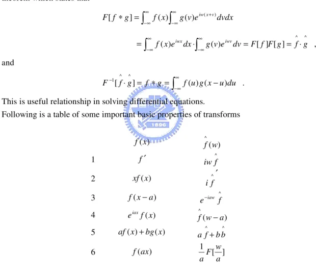
₋∞_∞ = ≡u w y u x y e dx y w u F[ ]( , ) ( , ) ( , ) iwx ^ .

A basic property of the Fourier transform is that the k th derivative _u( k) _with

,... 2 , 1 =

k transforms to an algebraic expression，that is

) , ( ) ( ) , ]( [ ^ y w u iw y w u F k = − k ,

confirming our comment that derivatives are transformed to multiplication. This formula is easily proved by integration by parts.