Formulations of Support Vector Machines: A Note from an
Optimization Point of View
Chih-Jen Lin
Department of Computer Science and Information Engineering, National Taiwan Uni-versity, Taipei 106, Taiwan
In this article, we discuss issues about formulations of support vector machines (SVM) from an optimization point of view. First, SVMs map training data into a higher- (maybe infinite-) dimensional space. Cur-rently primal and dual formulations of SVM are derived in the finite dimensional space and readily extend to the infinite-dimensional space. We rigorously discuss the primal-dual relation in the infinite-dimensional spaces. Second, SVM formulations contain penalty terms, which are dif-ferent from unconstrained penalty functions in optimization. Tradition-ally unconstrained penalty functions approximate a constrained problem as the penalty parameter increases. We are interested in similar properties for SVM formulations. For two of the most popular SVM formulations, we show that one enjoys properties of exact penalty functions, but the other is only like traditional penalty functions, which converge when the penalty parameter goes to infinity.
1 Introduction
The support vector machine (SVM) is a new and promising classification technique (for surveys of SVM, see Vapnik, 1995, 1998). Given training vec-tors xi ∈ Rn, i = 1, . . . , l in two classes and a vector y ∈ Rn such that yi∈ {1, −1}, the SVM requires the solution of the following quadratic pro-gramming problem (Boser, Guyon, & Vapnik, 1992):
P0: min
1 2hw, wi
yi(hw, φ(xi)i + b) ≥ 1, i = 1, . . . , l, whereh·, ·i is the inner product of two finite or infinite vectors.
Training vectors xiare mapped into a higher-dimensional space by the functionφ. In this new space, we seek a separating hyperplane hw, φ(x)i +
b= 0 with coefficients w and b such that all training vectors are separated.
Note that this higher-dimensional space can be finite or infinite. In this article, to stress the difference between finite and infinite inner products, we represent them as xTy andhx, yi, respectively.
If in a higher-dimensional space, data are still not separable, Cortes and Vapnik (1995) propose adding a penalty term CPli=1ξiin the objective func-tion, where C is a large, positive number:
PC: min 1 2hw, wi + C l X i=1 ξi yi(hw, φ(xi)i + b) ≥ 1 − ξi, ξi≥ 0, i = 1, . . . , l.
The technique of introducing variablesξican be traced back to, for example, Bennet and Mangasarian (1992) for linear programming formulations.
As PC becomes a problem with many (or infinite) variables, currently the standard method (see, for example, Cortes & Vapnik, 1995, and Vapnik, 1995, 1998) for solving problem PCis through the following dual, which is a finite problem with l variables:
DC: min
1 2α
TQα − eTα
yTα = 0, 0 ≤ αi≤ C, i = 1, . . . , l,
where Qij ≡ yiyjhφ(xi), φ(xj)i and e is the vector of all ones. If α is a so-lution of(DC), w ≡
Pl
i=1yiαiφ(xi) is a solution of problem PC. Usually K(xi, xj) ≡ hφ(xi), φ(xj)i is called the kernel. Although φ(x) is in a very high-dimensional space, if a specialφ is used, K(xi, xj) is finite and can be easily calculated. Algorithms for solving DCcan be seen in, for example, Sch ¨olkopf, Burges, and Smola (1998). Similarly, the dual of problem P0is as
follows: D0: min 1 2α TQα − eTα yTα = 0, αi≥ 0, i = 1, . . . , l.
However, in the above references, the derivation of DCwas through the standard convex analysis in finite-dimensional spaces. Note thatφ(x) and
w can be vectors in an infinite-dimensional Hilbert space. Since properties
of convex analysis in finite spaces may not always hold in infinite spaces, we must be careful with any generalization. In this article, all results are derived for infinite-dimensional formulations.
The first issue is on the relation between PCand DC: C≥ 0. For example, we may ask whether it might happen that P0has an optimal solution but D0
is not solvable. Note that it is possible that a convex programming problem has a lower bound on all objective values but has no feasible points achieving this bound. In section 2, we show that P0and D0are either both solvable
or P0is infeasible and D0is unbounded. In addition, PCand DC, C> 0 are both solvable.
Cortes and Vapnik (1995) and, more recently, Friess, Cristianini, and Campbell (1998) offer a different SVM formulation:
¯PC: min12hw, wi + C2 Pli=1ξi2 yi(hw, φ(xi)i + b) ≥ 1 − ξi, i= 1, . . . , l. ¯DC min12αT¡Q+ I C ¢ α − eTα yTα = 0, αi≥ 0, i= 1, . . . , l.
Here I is the identity matrix. Using similar techniques, we show that both ¯PCand ¯DC, C> 0 are always solvable.
The second topic of this article is the penalty parameter. In PC(or ¯PC), the penalty term CPli=1ξi(orC2Pli=1ξi2) is added to reduce the occurrence of incorrectly classified data. Note that such an approach is different from traditional penalty functions, which modify constrained problems to un-constrained ones. As the penalty parameter goes to infinity, the solutions of this sequence of unconstrained problems approximate a solution of the original problem. Here we are interested in similar properties for SVM for-mulations. In section 3, we show that for PC, after C is greater than a certain number, all solutions of PCare a solution of P0. In other words, PCis like an exact penalty function approach. On the other hand, this result may not hold for ¯PCbut as C→ ∞, solutions of ¯PCstill converge to a solution of P0.
We hope that we demonstrate a framework on optimization properties of SVM formulations. Hence, when new formulations are proposed, similar tools and techniques can be applied without many modifications. Finally we make conclusions and discussions in section 4.
2 Primal-Dual Relation of SVM Formulations
For the discussion in the rest of this article, we need the following theorem, which shows the necessary and sufficient optimality conditions of a convex optimization problem. This is an extension of the KKT condition in finite-dimensional spaces. Note that the standard necessary condition usually requires some constraint qualifications (e.g., Slater condition). However, for problems with linear constraints, such an assumption is not necessary. Theorem 1. Consider an optimization problem
min f(x) s.t. hvi, xi − bi≥ 0, i = 1, . . . , l,
where x∈ X, a Hilbert space, vi ∈ X, i = 1, . . . , l and bi ∈ R, i = 1, . . . , l. If f is a real convex and differentiable function, then a feasible element x is an optimal solution if and only if there exist real numbersλ1, . . . , λlsuch that
∇ f (x) − λ1v1− · · · − λlvl= 0
Proof. The necessary condition when constraints are linear can be seen in, for example, Girsanov (1972, theorem 11.3). The sufficient condition does not require any constraint qualification. An example of proof can be seen in corollary 1.1 of Barbu and Precupanu (1986, chap. 3).
Note that the definition of∇ f (x) here is in the sense of Frechet differen-tiability. Theorem 1 can be extended to linear equality constraints as a linear equality can be written as two linear inequalities.
Then the following theorem shows the relation between P0and D0: Theorem 2. For problems P0and D0, only one of the following two situations
can happen:
P0solvable and D0solvable,
P0infeasible and D0unbounded.
On the other hand, PCand DC, C> 0, are both solvable.
Proof. First we prove that if D0is solvable, P0is solvable. Suppose that an
optimal solution of D0isα, by theorem 1 (necessary condition), there exists
a b such that
αi(Qα − e − by)i= 0, i = 1, . . . , l, and Qα − e − by ≥ 0.
By defining w≡Pli=1αiyiφ(xi), we have (w, b) which satisfies the optimality condition of P0. From theorem 1 (sufficient condition),(w, b) is an optimal
solution of P0. Hence P0is solvable.
Next we show that if P0is feasible, D0is solvable. Consider the following
problem: max α≥0 ( inf w,b " 1 2hw, wi − l X i=1 αi(yi(hw, φ(xi)i + b) − 1) #) . (2.1)
When yTα = 0, infw,b[12hw, wi −Pli=1αi(yi(hw, φ(xi)i + b) − 1)] has a global minimum at w=Pli=1αiyiφ(xi) (see, for example, Debnath & Mikusinski, 1999, example 9.3.3). Thus equation 2.1 is equivalent to D0. It can be clearly
seen that if P0 is feasible with any feasible solution w∗, 12hw∗, w∗i is an
upper bound of equation 2.1. That is,−12hw∗, w∗i is a lower bound of D0.
From corollary 27.3.1 of Rockafellar (1970), any feasible bounded finite-dimensional space quadratic convex function over a polyhedral attains at least an optimal solution. Since D0 is always feasible, we know that it is
solvable.
Furthermore, because a feasible P0 implies a solvable D0 and a
is attained. Therefore, we conclude that there are only two possible situa-tions:
P0solvable and D0solvable.
P0infeasible and D0unsolvable.
We then use the same property that if D0is bounded, it is solvable. Therefore,
D0unsolvable means D0is unbounded, so the proof is complete.
Since PCand DC, C> 0, are both feasible, by the same arguments above, they are both solvable.
Using a similar method, we can prove that ¯PC and ¯DC are also both solvable.
3 Penalty Parameters
In PC (or ¯PC), the penalty term C Pl
i=1ξi(or C2 Pl
i=1ξi2) is used to reduce the occurrence of wrongly classified data. This is different from the penalty approach in mathematical programming. Originally this method approx-imates a constrained problem by unconstrained minimization. When the penalty parameter is large enough, minima of unconstrained problems are close to a solution. Hence it is important to know that if P0 is separable,
how close a solution of PCis to a solution of P0as C increases. This can be a
criterion to judge the appropriateness of using the penalty term and will be the main topic of this section. First we prove the following technical lemma: Lemma 1. For any C≥ 0, the vector w of optimal solutions of PCis unique.
Proof. Assume that(w, b, ξ) and ( ¯w, ¯b, ¯ξ) with w 6= ¯w are both optimal solutions of PC. For any 0≤ α ≤ 1, ( ˆw, ˆb, ˆξ) = α(w, b, ξ) + (1 − α)( ¯w, ¯b, ¯ξ) is feasible to PC. Therefore, 1 2h ˆw, ˆwi + C l X i=1 ˆξi≥ 1 2hw, wi + C l X i=1 ξi= 1 2h ¯w, ¯wi + C l X i=1 ¯ξi. (3.1) Note that equation 3.1 can be treated as two inequalities. By multiplying the first part byα and the second part by (1 − α),
1 2α 2hw, wi + α(1 − α)hw, ¯wi +1 2(1 − α) 2h ¯w, ¯wi ≥1 2αhw, wi + 1 2(1 − α)h ¯w, ¯wi. Thus, α(1 − α)hw − ¯w, w − ¯wi ≤ 0, ∀0 ≤ α ≤ 1.
Since w− ¯w is in a Hilbert space, w − ¯w = 0. This causes the contradiction, so w must be unique.
For other variables such as b andξ of PCandα of DC, there are always ex-amples where multiple solutions occur. Next we present a relation between solutions of PC, C > 0 and those of P0.
Theorem 3. If P0is solvable, there is a C∗such that for all C≥ C∗, any solution
(w, b) of P0is a solution of PC.
Proof. If(w, b) is a solution of P, by theorem 1, there are α and b such that
w= l X i=1 yiαiφ(xi), yTα = 0, α ≥ 0 αi(yihφ(xi), wi + b − 1) = 0, i = 1, . . . , l.
Let C∗> max(αi). For all C > C∗, we can setξ = 0 and obtain w= l X i=1 yiαiφ(xi), yTα = 0 αi(yihφ(xi), wi + b − 1 + ξi) = 0 0≤ αi≤ C, ξi(C − αi) = 0, i = 1, . . . , l.
Therefore, from theorem 1,(w, b, ξ) is also a solution of PC.
Theorem 3 proves a property similar to exact penalty functions. That is, after the penalty parameter is large enough, any solution of the origi-nal problem is also a solution of peorigi-nalty functions. However, according to Di Pillo (1994), they are only weak exact penalty functions, though most early literature on penalty functions studied this result. Since the penalty approach is an attempt to solve P0, it is more important to study the
con-verse property, which ensures that solutions of PCare solutions of P0. It is
shown in the following theorem and corollary:
Theorem 4. If P0is solvable, there is a C∗such that for all C≥ C∗, any solution
(w, b, ξ) of PCsatisfies thatξ = 0 and (w, b) is a solution of P0.
Proof. Consider any C∗ such that theorem 3 holds and assume(w, b) is a solution of P0. From theorem 3,(w, b, 0) is also an optimal solution of PC. Now if we solve PCand obtain( ¯w, ¯b, ¯ξ), from lemma 1, ¯w = w. Therefore,
1 2h ¯w, ¯wi + C l X i=1 ¯ξi≤ 1 2hw, wi.
Corollary 1. If P0is solvable and C∗≡ min ½ max i=1,...,lαi| α is a solution of D0 ¾ ,
each of PC, C < C∗ has a different solution w from the solution of P0. On the
contrary, PC, C ≥ C∗has the same solution w as that of P0.
Proof. When C≥ C∗, the result is given by theorem 4. For the case of C< C∗, assume there is a PCwith a solution(wC, bC, ξC) such that wCis also part of a solution of P0. If(w, b) is a solution of P0,(w, b) is feasible to PC, so
1 2hwC, wCi + C l X i=1 (ξC)i≤1 2hw, wi.
This impliesξC= 0. Hence any solution of DCis also a solution of D0. Since
C< C∗, this contradicts the definition of C∗.
As we show only that vectors w are different, when C< C∗, it is still possible to obtain the same separating hyperplane. Note thathw, φ(x)i +
b= 0 is the hyperplane so any α(w, b), α 6= 0, are appropriate coefficients.
However, when C< C∗, the separating plane generated by PCcan also be very different from that of P0. For example, consider a problem with three
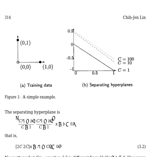
points, 0, 1, and 100, where 0 is in the first class, 1 and 100 are in the other class, and K(xi, xj) = xTixj. When C ≥ 2, α = [2, 2, 0] and the hyperplane is 2x− 1 = 0. When 1 ≤ C ≤ 2, α = [C, C, 0] and w = C. As b can be any number that satisfies−1 ≤ b ≤ 1 − C, b = −C/2 can be a choice. Therefore, 2x− 1 = 0 can still be a solution. However, when C becomes smaller, the hyperplane starts moving toward the training point 100. In addition, the distance between two planes hw, xi + b = ±1 becomes very large. This shows that if small Cs are used, some careful analysis should be conducted. Next we switch the target to ¯PCand ¯DC. Interestingly they are not like exact penalty functions. In the following example, we show that no matter how large C is, solutions of ¯PCare not solutions of P0. In Figure 1a, there are
three training vectors in two different classes. If Qij= yiyjxTixj, the optimal separating hyperplane for P0is [2 2]x− 1 = 0. The optimality condition of
¯PCis 1 C 0 0 0 1+C1 0 0 0 1+C1 αα12 α3 + b −11 1 − 11 1 = λλ12 λ3 .
At the solution, all three vectors are support vectors soλ = 0. Solving the above equation with yTα = 0 obtains
b= C− 1
−C − 3, α1= (1 + b)C, α2= α3= (1 − b)C
C+ 1 =
2C
Figure 1: A simple example.
The separating hyperplane is · C(1 − b) C+ 1 C(1 − b) C+ 1 ¸ x+ b = 0, that is, [2C 2C]x+ (1 − C) = 0. (3.2)
No matter what C is, equation 3.2 is different from [2 2]x− 1 = 0. However, it can be seen in Figure 1b that as C→ ∞, equation 3.2 approaches [2 2]x − 1 = 0. In the following theorems we show that ¯PC has properties of only traditional penalty functions. That is, as C→ ∞, solutions of ¯PCapproach solutions of P0.
Lemma 2. Let(wCj, bCj, ξCj) be a solution of ¯PCj,αCj be the solution of ¯DCj,j= 1, 2, . . ., and assume limj→∞Cj= ∞. If P0is solvable and limj→∞αCjexists, then limj→∞wCjexists and is the solution of P0.
Proof. From the optimality condition (see theorem 1) of ¯DC,αCj = CξCj. Since limj→∞αCj exists, limj→∞ξCj = 0. As wCj = Pli=1yi(αCj)iφ(xi) and limj→∞αCj exists, limj→∞wCjexists and we can denote it as w. Note that
max
i: yi=1(1 − (ξCj)i− hwCj, φ(xi)i) ≤ bCj ≤ mini: yi=−1(−1 + (ξCj)i+ hwCj, φ(xi)i).
As Cj→ ∞, limj→∞ξCj= 0 so max
Hence w is feasible to P0. Furthermore, as P0is solvable, we can assume ¯w is
a solution. Since ¯w is feasible to all ¯PC, C > 0 and wCjis the optimal solution of ¯PCj, we have
1
2hwCj, wCji ≤ 1 2h ¯w, ¯wi.
As j→ ∞,12hw, wi ≤12h ¯w, ¯wi. Hence limj→∞wCj = w is an optimal solution of P0.
Theorem 5. Let (wC, bC, ξC) be a solution of ¯PC. If P0 is solvable, then
limC→∞wCexists and is the solution of P0.
Proof. First we prove that{αC | C ≥ ²} is bounded, where αCis a solution of DCand² is any positive number. If ¯α is a solution of D0,¯α is feasible to
¯DCandαCis feasible to D0, so 1 2¯α TQ¯α − eT¯α ≤ 1 2α T CQαC− eTαC ≤1 2α T C µ Q+ I C ¶ αC− eTαC≤ 1 2¯α T µ Q+ I C ¶ ¯α − eT¯α.
The above formula provides lower and upper bounds on12αCT(Q +CI)αC− eTα
Cwhen C≥ ² > 0. From the optimality condition (see theorem 1) of ¯DC, −1 2α T C µ Q+ I C ¶ αC+ eTαC= 1 2α T C µ Q+ I C ¶ αC.
Hence12αTC¡Q+CI¢αCis bounded and so as eTαC. SinceαC≥ 0, this implies that{αC} is bounded after C is large enough.
Since{αC| C ≥ ²} is bounded, there exists a convergent sequence {αCj}. From lemma 2, limj→∞wCj exists, where wCj is part of a solution of ¯PCj. If limC→∞wC 6= w, there is a sequence {wCk} and δ > 0 such that kwCk − wk ≥ δ, for all k = 1, 2, . . .. However, {αCk} is bounded so we can find a subsequence of{αCk} which satisfies conditions of lemma 2. Hence this subsequence converges to a solution of P0, that is, w. This contradicts the
assumption thatkwCk− wk ≥ δ, ∀k. Therefore, limC→∞wC= w
4 Conclusions
Through the use of optimization techniques, we have a better understanding about formulations of SVMs. This work can be a good example of analyzing future SVM formulations by optimization techniques.
SVM formulations are very simple convex quadratic problems in Hilbert spaces. Thus we can use the simple Wolfe dual (see equation 2.1) to derive
the primal-dual relation instead of using the standard conjugate duality. For different SVM formulations, the results of theorem 2 could be quite different. For example, for the newν-SVM proposed by Sch¨olkopf, Smola, Williamson, and Bartlett (2000), the primal problem can be unbounded while the dual problem can be infeasible (see Crisp & Burges, in press, and Chang & Lin, 2000).
Acknowledgments
This work was supported in part by the National Science Council of Taiwan, grant NSC-88-2213-E-002-097. The author thanks Jorge Mor´e for pointing him to Di Pillo (1994) and some helpful discussions. He also thanks Chih-Wei Hsu and Steve Wright for their comments.
References
Barbu, V., & Precupanu, T. (1986). Convexity and optimization in banach spaces. Dordrecht: D. Reidel.
Bennett, K. P., & Mangasarian, O. L. (1992). Robust linear programming dis-crimination of two linear inseparable sets. Optimization Methods and Software 1, 23–34.
Boser, B., Guyon, I., & Vapnik, V. (1992). A training algorithm for optimal mar-gin classifiers. In Proceedings of the Fifth Annual Workshop on Computational Learning Theory.
Chang, C.-C., & Lin, C.-J. (2000). Some analysis onν-support vector classification (Tech. Rep.) Taipei, Taiwan: Department of Computer Science and Informa-tion Engineering, NaInforma-tional Taiwan University.
Cortes, C., & Vapnik, V. (1995). Support-vector network. Machine Learning, 20, 273–297.
Crisp, D. J., & Burges, C. J. C. (In press). A geometric interpretation ofν-svn classifiers. In Advances in neural information processing systems. Cambridge, MA: MIT Press.
Debnath, L., & Mikusinski, P. (1999). Introduction to Hilbert spaces with applications (2nd ed.). San Diego: Academic Press.
Di Pillo, G. (1994). Exact penalty methods. In I. Ciocco (Ed.), Algorithms for continuous optimization. Dordrecht: Kluwer.
Friess, T.-T., Cristianini, N., & Campbell, C. (1998). The kernel Adatron algo-rithm: A fast and simple learning procedure for support vector machines. In Proceedings of the 15th Intl. Conf. Machine Learning. San Mateo, CA: Morgan Kaufmann.
Girsanov, I. V. (1972). Lectures on mathematical theory of extremum problems. Berlin: Springer-Verlag.
Rockafellar, R. T. (1970). Convex analysis. Princeton, NJ: Princeton University Press.
Sch ¨olkopf, B., Burges, C. J. C., & Smola, A. J. (Eds.) (1998). Advances in kernel methods—Support vector learning. Cambridge, MA: MIT Press.
Sch ¨olkopf, B., Smola, A., Williamson, R. C., & Bartlett, P. L. (2000). New support vector algorithms. Neural Computation, 12, 1083–1121.
Vapnik, V. (1995). The nature of statistical learning theory. New York: Springer-Verlag.
Vapnik, V. (1998). Statistical learning theory. New York: Wiley. Received September 20, 1999; accepted April 12, 2000.