國
立
交
通
大
學
多媒體工程研究所
碩
士
論
文
結合多層次解析度之貼圖為主的
特徵追蹤演算法
Multi-resolution Texture-based Feature Tracking
in Large Time-varying Volume Visualization
研 究 生:傅光暐
指導教授:莊榮宏 教授
王才沛 教授
結合多層次解析度之貼圖為主的特徵追蹤演算法
Multi-resolution Texture-based Feature Tracking
in Large Time-varying Volume Visualization
研 究 生:傅光暐 Student:Kuang-Wei Fu
指導教授:莊榮宏 Advisor:Jung-Hong Chuang
王才沛 Tsai-Pei Wang
國 立 交 通 大 學
多 媒 體 工 程 研 究 所
碩 士 論 文
A ThesisSubmitted to Institute of MultimediaEngineering College of Computer Science
National Chiao Tung University in partial Fulfillment of the Requirements
for the Degree of Master
in
Computer Science
Nov. 2008
Hsinchu, Taiwan, Republic of China
結合多層次解析度之貼圖為主的特徵追蹤演算法
學生: 傅光暐 指導教授: 莊榮宏 博士 王才沛 博士 國立交通大學 多媒體工程研究所 摘要 我們提出了一個擁有多層次解析度架構 (multi‐resolution hierarchy) 之有效 率的貼圖特徵萃取及追蹤演算法 (feature extraction and tracking algorithm)。 在 前處理運算時,我們套用蓋式濾波器 (Gabor filter) 來計算多層次架構下每層解 析度的貼圖特徵係數 (texture attributes)。 各層次之特徵係數可以以其在空間上 的關係,架構成一個貼圖取樣層次架構。 在執行運算時,我們使用新的基於層 次架構的特徵追蹤演算法。 由於層次架構中,上下層之間有著空間上的關係, 當我們從貼圖取樣架構之頂端追蹤至底層時,上層之追蹤結果,能夠幫助下層之 節點決定其追蹤範圍。 在我們的結果中可以顯示多層次架構的方法明顯的改善 傳統貼圖為主的特徵追蹤演算法之效率,並且此種架構也能夠良好的適應不同類 型的資料及多目標追蹤 (multi‐target tracking)。Multi-resolution Texture-based Feature Tracking in Large
Time-varying Volume Visualization
Student: Kuang-Wei Fu
Advisor: Dr. Jung-Hong Chuang
Dr. Tsai-Pei Wang
Institute of Multimedia Engineering
College of Computer Science
National Chiao Tung University
ABSTRACT
We proposed an efficient texture-based feature extraction and tracking algorithm with multi-resolution hierarchy. In the preprocessing step, texture attributes are computed by Gabor filter-ing at each level of multi-resolution hierarchy. With spatial coherence, these attributes are builded as a texture sample hierarchy. In the run-time, a hierarchical feature tacking algorithm is applied. From root to leaves of the texture sample hierarchy, we use the parents tracking result to help children decide their tracking window. We demonstrate how this structure can perform more efficient tracking in texture-based datasets. The tracking algorithm is also adapted with multi-target feature.
Acknowledgments
I would like to thank my advisors, Professor Jung-Hong Chuang, and Tsai-Pei Wang for their guidance, inspirations, and encouragement. I am grateful to Horng-Shyang Liao for his comments and advices. Thanks to my colleagues in CGGM lab.: Yueh-Tse Chen, Ying-Tsung Li, Chih-Hsiang Chang, Hsin-Hsiao Lin, Ta-En Chen, Jau-An Yang, Cheng-Min Liu, and Hong-Xuan Ji for their assistances and discussions. I also want to thank senior colleagues, Chih-Wen Chang, Yu-Shuo Lio, Chia-Lin Ko, Ya-Ching Chiu,and Yung-Cheng Chen. It is pleasure to be with all of you in the pass two years. Lastly, I would like to thank my parents for their love, and support.
Contents
1 Introduction 1 1.1 Thesis Overview . . . 2 1.2 Contribution . . . 3 1.3 Outline . . . 3 2 Background 4 2.1 Multi-resolution Rendering . . . 42.2 Time-varying Data Representation . . . 6
2.3 Feature Extraction and Tracking . . . 6
3 Texture-based Feature Tracking 10 3.1 System Overview . . . 11
3.2 Texture Feature Analysis . . . 13
3.2.1 Texture Sampling . . . 13
3.2.2 Texture Attributes Calculation . . . 14
3.3 Hierarchical Feature Tracking . . . 17
3.3.1 Algorithm . . . 17
3.3.2 Feature Sample Comparison . . . 20 4 Result 24
4.1 Example Data Sets . . . 24
4.2 Preprocessing Result . . . 25
4.3 Run Time Tracking Result . . . 26
4.4 Discussion . . . 29
5 Conclusion 31 5.1 Summary . . . 31
5.2 Future Work . . . 32
5.2.1 Object-based Feature Extraction . . . 33
5.2.2 Hybrid Method Approach . . . 34 Bibliography 37
List of Figures
2.1 The evolutionary events that a feature may experience. . . 8 3.1 The structure of our system . . . 11 3.2 Here we show two levels of hierarchical sampling. Pink crosses stand for the
uniform sampling samples, and the blue crosses are added to increase the coor-dinate flexibility. . . 14 3.3 (a) A slice view of a 3D Gabor filter. (b) An iso-surface view of a 3D Gabor
filter. Here σx0 = σy0 = σz0, which makes the Gaussian envelope symmetric
and the iso-surfaces in (b) circle- shaped; the normal of these iso-surfaces are (1, 1, 1), because U = V = W . . . 15 3.4 Three different scales of Gabor filter kernel. The kernel size is set to be 8x8. . . 16 3.5 (a) Filter direction in 2D. (b) Filter direction in 3D as a hemisphere . . . 16 3.6 As we choose the target from left timestep, a brute force algorithm is apply until
we find the best match. . . 18 3.7 As we choose a tracking window, we can reduce the comparisons we need. . . 18 3.8 With wavelet transform, every parent node can be separate to 4 child node in 2D 19 3.9 Parent node can decide a 6x6 tracking window size. . . 20 3.10 The tracking process of one texture sample hierarchy. . . 21 3.11 Conventional data motions. . . 22
3.12 The figure on the left is the example drawing, which the yellow bar stand for the peak of the filter kernel. From top to down stand for the filter bank of a data in 2D, which has 4 different directions. In the comparison step, if we don’t have the rotational comparison, then we can find that target and the Sample A is totally different on every filtered value. On the other hand, we can find that target(1) has the similar value with Sample B(2), target(2) is similar to
Sam-ple B(3), and so on. . . 23
4.1 The Vortex data set. . . 25
4.2 Tracking result. . . 26
4.3 Tracking result. . . 27
4.4 The grows of comparisons. . . 28
4.5 The grows of comparisons for two different tracking algorithm. . . 29
5.1 Hybrid method which texture-based tracking result as an object extraction pro-cess input. . . 34
5.2 Hybrid method which object-based extraction with texture-based correspon-dence test. . . 35
5.3 Hybrid method which texture-based tracking with motion pattern recognition. . 36
List of Tables
4.1 The data set used in our testing. . . 24 4.2 The samples at root level. . . 25
C H A P T E R
1
Introduction
Feature extraction and tracking is a very common approach to overcome the difficulty of effec-tive visualization of large datasets due to the complexity of illustrating multiple timesteps and clearly showing changes and variations over time. Instead of visualizing the entire data set at once, feature extraction process can help isolating the features of interest from the overall data so they can be more economically stored and examined, or presented more clearly to the user. When analyzing features of time-varying data, not only do they need to be extracted, but they need to be tracked through time.
Existing feature extraction and tracking techniques tend to fall into one of two categories: correspondence based approaches and high-dimensional multi-attributes approaches. In the cor-respondence based approaches, the features in each timestep are extracted separately and then correspond the extracted features in consecutive timesteps based on criteria such as position, size, orientation, or region overlap [24] [25] [27] [28] [29]. These approaches generally are fairly robust, but there are, however, several limitations. First, previous approaches assume a high and sufficient temporal sampling in which feature overlap in subsequent timesteps. Sec-ond, most algorithm assume that important features can be easily segmented. Another category is to use high-dimensional multi-attributes known as texture-based method. The local textural
1.1 Thesis Overview 2 information is extracted using several mathematical or statical calculation, and then compare the texture in the consecutive timesteps to find a best match. However, the performance of cal-culating texture attributes is influence by the texture size. Another problem comes out when tracking feature, without motion prediction the tracking process need lots of comparison to find the match, and it gets worse when a dataset grows bigger.
1.1
Thesis Overview
Our method is basically based on texture-based feature tracking combined with multi-resolution data hierarchy. With user choose region of interest (ROI), which decides the tracking target the feature information is extract and the tracking process can be done by following the target movement at the rest of the timesteps.
The feature is defined by the data distribution on a texture in texture-based feature track-ing. These data distribution information are calculated by lots of mathematical and matrix calculation to extract as texture feature. The texture feature information have to be calculated after user’s target input, and the loading of feature extraction slows down the tracking and rendering performance. With pre-calculated texture feature information, we can speed up the performance, but increase the difficulties of tracking target, because the correctness can not be ensured.
We propose multi-resolution hierarchy method to ensure tracking correctness and perfor-mance. We sample and extract information at every level of resolution. As we switch the level from top to down within the resolution, the spatial coherence and the data distribution properties increase the tracking process correctness. On the other hand, the tracking structure is similar to rendering hierarchy and will not increase the rendering loading.
1.2 Contribution 3
1.2
Contribution
The contributions of this thesis can be summarized as :
• We proposed a hierarchical feature tracking algorithm, which – Speed up the texture-based feature tracking processes. – Spatial coherence is guaranteed.
– The information of the region probability is easily obtained within the tracking processes.
1.3
Outline
The rest of the thesis is organized as follows: Chapter 2 gives the literature review, the back-ground of time-varying volume rendering and feature tracking algorithm for volume dataset. Chapter 3 presents the Texture-based hierarchical feature tracking and hybrid method we pro-posed for object-based feature picking, which includes algorithms and implementation details. Chapter 4 shows our experimental result from our approach. In the end, conclusions and future work are discussed in Chapter 5.
C H A P T E R
2
Background
This chapter introduces the related work about feature extraction and tracking in volume dataset. It is divided into three parts: the first part is the multi-resolution rendering technique. The sec-ond part describes the structure and representation of the time-varying volume dataset. Finally, different approaches of the feature extraction and tracking in 3D volumetric data are introduced.
2.1
Multi-resolution Rendering
The idea of multi-resolution volume rendering algorithms is to provide a spatial hierarchy to adapt the data resolution to render the interesting or important regions with higher accuracy, while other regions are rendered with lower accuracy. LaMar et al. [17] describe an octree-based multi-resolution approach for interactive volume rendering. They filter the volume to create levels-of-detail in an octree structure. They propose the use of spherical shells to reduce visual artifacts for 3D texture mapping. A similar technique was proposed by Boada et al. [3]. Their hierarchical representation benefits nearly homogeneous regions and regions of lower interest. Weiler et al. [36] address the avoidance of discontinuity artifacts between different
2.1 Multi-resolution Rendering 5 levels of detail. Their approach allows consistent interpolation between levels. These multi-resolution techniques can handle volume data sets that do not fit completely into the texture memory of the graphics hardware. However, the data must still fit into the main memory. Guthe et al. [11] improved on this by using wavelet representation. They recursively apply wavelet transform to compress the data and construct a multi-resolution hierarchical wavelet representation. Their approach is able to render walkthroughs of large data sets in real time on a conventional PC.
Multi-resolution volume rendering provides a data hierarchy that supports level-of-detail (LOD). There are several types of criteria for the LOD selection. These LOD selection methods can be classified into four types. We give a brief overview to these LOD selection methods:
1. View-dependent criterion: This is a general criterion that takes the view- dependent fac-tors into account. According to the position of viewer, it will let the regions that are closer to the viewer or the regions with larger projected screen area have higher resolution [11] [17].
2. Region-of-interest: This criterion depends on the user-specified region- of-interest (ROI) to decide LOD selection [20] [21]. Usually there is a 3D bounding box to represent the ROI. The regions inside the ROI bounding box have higher resolution.
3. Data error metric: The data error metric calculates the error (usually the mean squared error) between the low resolution data block and the corresponding original volume data. Then, the LOD selection is decided by letting each subvolume satisfy the user-specified error tolerance [26] [32].
4. Image-based quality metric: The image-based quality metric evaluates the contribution of multi-resolution data blocks to the final image. The LOD selection algorithm tries to choose a set of blocks that generate images of best visual quality [18] [33] [34].
2.2 Time-varying Data Representation 6
2.2
Time-varying Data Representation
In the volume rendering field, some dataset will evolution as the time goes by, we called time-varying data. In this kind of dataset, the temporal evolution is as important as the spatial reso-lution problem. Shen et al. [26] proposed time space partitioning (TSP) tree that captures both the spatial and temporal coherence of the underlying data. It allows the user to request spatial and temporal data resolutions independently with separate error tolerances. Wang and Shen fur-ther utilized wavelet transform to propose wavelet-based time-space partitioning (WTSP) tree method [32]. They first build a wavelet tree hierarchical representation [11] for each individual time step. Then for the high-pass filtered coefficients from the corresponding spatial node along the time axis, they apply 1D wavelet transform to form a binary time tree. Although WTSP tree method supports flexible spatial-temporal multi-resolution data browsing, their hierarchical 1D wavelet compression of the spatial node along the time axis is not suitable for interactive play-back. Ko et al. [16] presented framework that combines the multi-resolution hierarchy with video-based compression to manage and render large scale time-varying data. The method first constructs the wavelet tree hierarchy for each individual time step, and then applies motion-compensation-based prediction. The proposed approach breaks the hierarchical decompression dependency in the conventional hierarchical wavelet representation methods, and allows a more efficient reconstruction of data along the time axis.
2.3
Feature Extraction and Tracking
Most of the research in time-varying volume visualization has focused on rendering perfor-mance of storage issues. Samtaney et al. [25] were the first to identify computer vision feature extraction techniques and to extend them from the 2D image domain to the 3D volume domain. Feature extraction and tracking is a well established technique for analyzing time-varying data in 2D image domain, such as video analysis [4] [35], computer vision [30] [8] [14]. Scientists also wants to track features in 3D volume domain to observe, analyze the feature information.
2.3 Feature Extraction and Tracking 7 In the feature tracking domain, several problems have to be solved: feature definition, feature extracting process, and feature tracking algorithm.
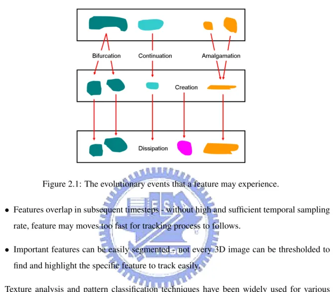
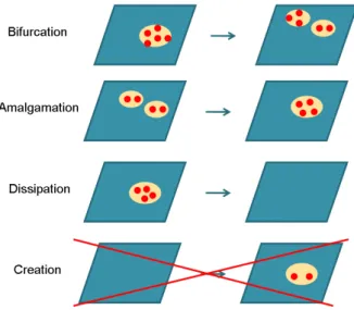
Computational fluid dynamic(CFD)simulations figured heavily in early research of visual-ization and feature extracting and tracking of time-varying data. In the field of CFD data, the feature usually defines on the fluid itself as an object, that is separate the fluid and the air which means no data. We use several extraction technique, such as segmentation [27], volume inter-vals [10] to isolates the features to track for each timestep, then associate them through time. There are various algorithms proposed previously [22]. Based on how the topological tructure of a local feature evolves over time, one of the following events can occur: (see Fig 2.1)
• Continuation: An object continues to the next time step, with possible shape deformation and change of position, orientation, etc.
• Creation: A new feature starts to appear. • Dissipation: A feature disappears.
• Bifurcation: A feature splits into several parts.
• Amalgamation: Several features merge into a single one.
Silver and Wang [28] [29] presented a feature tracking technique that extracts features, organizes them into an octree structure, and tracks the thresholded, connected components in subsequent timesteps. Reinders et al. [24] proposed a tracking technique that uses feature attributes, such as position, mass, and size to solve the feature correspondence problem between frames. Ji et al. [15] introduced a method to track local features from time-varying data by using higher-dimensional iso-surfacing. Tzeng and Ma [31] proposed a technique to extract and track features in time-varying data by using a machine learning module capable of learning from the transfer function, with extracts the user wishes the knowledge can be applied to the visualization pipeline in subsequent volumes.
There are, however, several limitations to existing feature tracking techniques for object-based time-varying volumetric data:
2.3 Feature Extraction and Tracking 8
Figure 2.1: The evolutionary events that a feature may experience.
• Features overlap in subsequent timesteps - without high and sufficient temporal sampling rate, feature may moves too fast for tracking process to follows.
• Important features can be easily segmented - not every 3D image can be thresholded to find and highlight the specific feature to track easily.
Texture analysis and pattern classification techniques have been widely used for various tasks in the computer vision, computer graphics and visualization fields. With extracting texture properties to track, features don’t have to overlap in subsequent timesteps. In some scientific calculation datasets, object-based feature is also not easy to be extracted. There are several ways to extract texture-based feature, such as texture attributes [5] and image filtering [23]. For texture attributes method, several texture information have been calculated first, such as mean, standard deviation, and stored as a high-dimensional feature vector. The same features are expected to have the same feature vector members. Filtering method is applying convolution application to original image data, and with well designed filter kernel, the texture information can be extracted and compare between features.
Be-2.3 Feature Extraction and Tracking 9 longie et al. [1] used color- and texture-based image segmentation together with the expectation-maximization(EM) algorithm for retrieving similar images from a large image collection. Guan et al. [9] used texture-based techniques for categorizing traditional Chinese painting images. In the medical imaging field, Xu et al. [38] proposed a 3D texture feature approach to classify and differentiate lung CT images. Quan et al. [23] used a tunable 3D Gabor filter bank, to extract-ing the taggextract-ing sheets in tagged cardiac MR images, and trackextract-ing their displacement durextract-ing the heart cycle. In the field of scientific volumetric data visualization, Caban et al. [5] proposed a texture-based feature tracking technique capable of tracking multiple features over time by analyzing local textural properties and finding correspondent properties in subsequent volumes. They calculate multiple texture properties, such as mean, variance, co-occurrence matrix, run-length matrix, as a high-dimensional feature vector. With comparisons between feature vector of features, features can be tracked within timesteps.
C H A P T E R
3
Texture-based Feature
Tracking
Our development of a texture-based feature tracking algorithm in time-varying volume dataset is based on our observations. Texture-based feature extraction and tracking can work with different data format such as object, fluid, and vector field. In contrast, object-based method such as iso-surface is efficient with object-like dataset. Texture-based extraction needs lots of mathematical and matrix calculation, which increase with texture sizes, and is limited by the calculation efficiency.
In this chapter, we will introduce our system with two phases: texture information extrac-tion and hierarchical feature tracking. First we will define what feature is in texture-based feature tracking, and followed by an efficient hierarchical feature tracking algorithm to ensure the tracking performance and quality. Other rendering issues are mentioned bellow.
3.1 System Overview 11
3.1
System Overview
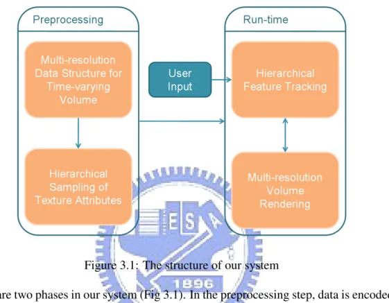
Figure 3.1: The structure of our system
There are two phases in our system (Fig 3.1). In the preprocessing step, data is encoded by a time-varying multi-resolution hierarchical structure. Then the texture attributes of the samples in each resolution level of each timestep are computed. At run time, the user choose a set of samples to be the tracking targets, and the target’s match is found by a hierarchical tracking algorithm. Finally, the volume is visualized by conventional texture-based volume rendering process.
The multi-resolution hierarchy use in our system is introduced by Ko et al.[16]. The struc-ture classify each timestep of the dataset as either an intra-coded frame (I-frame) or a predictive frame (P-frame). For an I-frame, the hierarchical wavelet transform is applied to construct the multi-resolution hierarchical wavelet representation. The high-pass filtered coefficients are en-coded and stored. For a P-frame, after the hierarchical wavelet transform has applied to build the hierarchical representation, a motion-compensation-based prediction of the low-pass filtered data is applied. The difference data and motion vectors are encoded and stored.
3.1 System Overview 12 After we build the multi-resolution hierarchy, the textural information have to be extracted. We apply uniform sampling in each level of resolution at each timestep. These samples’ texture attributes are computed and stored. We will get a hierarchical sampling of texture attributes at each timestep.
In tracking process, user choose a set of samples they focus at a certain timestep to be the target, and these samples’ displacement is tracked by texture-based comparison using their at-tributes. The numbers of the target sample and the candidates of each sample dominate the performance of the tracking process. We use multi-resolution structure to accelerate the track-ing process. Simply, because the numbers of samples in coarse resolution are small, and the matching results are found quick. As the resolutions increase, the matching results can adjust their correctness.
Finally, we apply conventional texture-based volume rendering technique. The level of detail is choose by region of interest combine with user’s view directions. We enforce a back-to-front traversal order of the resolution octree. For each block, the 3D texture is created and loaded into the texture memory. View-aligned slices are placed into blocks and render in back-to-front order. The alpha blending delivers the volume integrals along view rays for all pixels on the screen. After these steps, the matching results are marked by colored spheres in the scene.
3.2 Texture Feature Analysis 13
3.2
Texture Feature Analysis
In computer vision and image processing, textures are fundamental to identifying, character-izing, and comparing objects and regions with similar properties. Image differentiation can be achieved by characterizing similar properties and regular frequencies that occur in repeated patterns of specific images.
There are several ways to identify the texture properties for tracking, such as multiple at-tributes [5] and filter processing [23]. The multiple atat-tributes method uses several textural met-rics to identify and track features within dynamic time-varying data. Gabor filtering achieves optimal localization in both the spatial and the frequency domains, which makes it more suit-able for the texture tracking process. The Gabor filtering applications are basically a convolution calculation and the performance is effect by the kernel size and target texture size.
We use 3D Gabor filtering to calculate the texture properties combines with several first-order statistics, such as mean and texture displacement. In this chapter, we will introduce the filtering issue first, and then discuss the texture sampling for the pre-processing step. Finally, gives a global view of the pre-computed texture feature information calculation process to com-plete the system pre-processing step.
3.2.1
Texture Sampling
We calculate texture feature information in the preprocessing step of the system. Here we use uniform sampling with fifty percents data overlapping discussed below.
As we take the texture information of some local area as our features to track, the locations and sizes of the local area are what we have to decide. The Gabor filter application is a weighted summation of a local area and the filter kernel size is determine how big the local area is. After we decide the filter kernel size, which set to be 8 by our experiment, the size of the feature is settled. For uniform sampling of the volume dataset, we shift the filter kernel along three axis follow by x, y, and z. We use fifty percents data overlapping to increase the flexibility of the
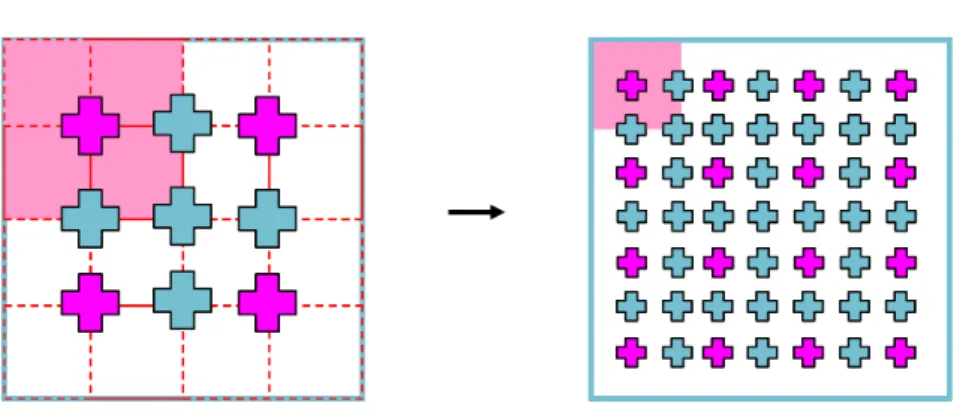
3.2 Texture Feature Analysis 14 tracking coordinate. See Fig 3.2 in 2D way.
Figure 3.2: Here we show two levels of hierarchical sampling. Pink crosses stand for the uniform sampling samples, and the blue crosses are added to increase the coordinate flexibility.
3.2.2
Texture Attributes Calculation
The filter responses that result from the application of a filter bank of Gabor filters can be used directly as texture features. At the feature comparison processes, we compare these filtered feature values to decide if these features are similar. The filter bank design is responsible for our feature tracking result, and have to be considered representative.
The 1D Gabor filter was first introduced by D. Gabor in 1946 [7]. It is basically a product of a Gaussian window and a complex sinusoid. 3D Gabor filter is a 3D extension of its 1D form and has been used in many image processing and computer vision field, such as 3D texture segmentation [6] [37] [19], motion analysis [2], object recognition [12], and medical image analysis [23]. If we extend the 1D function to 3D, we get
h(x, y, z) = g(x0, y0, z0) · s(x, y, z) (3.1) where g(x0, y0, z0) is a 3D Gaussian envelope, and s(x, y, z) is a complex sinusoid function, i.e.,
g(x0, y0, z0) = 1 (2π)32σx0σy0σz0 e− 1 2[( x0 σ x0 )2+(y0 σ y0 )2+(z0 σ z0 )2] , (3.2) s(x, y, z) = exp[−j2π(U x + V y + W z)], (3.3)
3.2 Texture Feature Analysis 15 In Equation 3.2: The standard deviation σ of the Gaussian envelope determines the effective size of the surrounding of a voxel in which weighted summation takes place. Note that σx0 ,
σy0 and σz0 may not be the same. Thus the shape of this Gaussian envelope can be an ellipsoid.
(x0, y0, z0)T = R × (x, y, z)T are the rotated coordinates of the Gaussian envelope. R is a
rotation matrix. Here in our system, we use a sphere-shaped 3D Gaussian envelope, which has a constant value of σ set to be 5 by our experiment and for sphere-like filter no rotation is needed. We can reformulate the equation as
g(x, y, z) = 1 (2π)32σ3
e−12[
x2+y2+z2
σ2 ], (3.4)
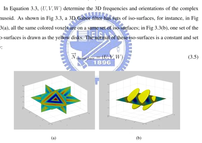
In Equation 3.3, (U, V, W ) determine the 3D frequencies and orientations of the complex sinusoid. As shown in Fig 3.3, a 3D Gabor filter has sets of iso-surfaces, for instance, in Fig 3.3(a), all the same colored voxels are on a same set of iso-surfaces; in Fig 3.3(b), one set of the iso-surfaces is drawn as the yellow disks. The normal of these iso-surfaces is a constant and set by:
− →
Nisosurf ace = (U, V, W ) (3.5)
(a) (b)
Figure 3.3: (a) A slice view of a 3D Gabor filter. (b) An iso-surface view of a 3D Gabor filter. Here σx0 = σy0 = σz0, which makes the Gaussian envelope symmetric and the iso-surfaces in
(b) circle- shaped; the normal of these iso-surfaces are (1, 1, 1), because U = V = W
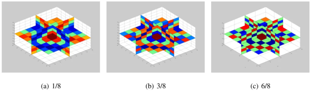
3.2 Texture Feature Analysis 16 choose 3 different scale which set to be n1, n3,and n6, where n is determined by filter kernel size to increase the discriminate ratio of feature tracking (see Fig 3.4).
(a) 1/8 (b) 3/8 (c) 6/8
Figure 3.4: Three different scales of Gabor filter kernel. The kernel size is set to be 8x8. The sinusoid is symmetry, and in order to achieve rotational invariance, every sample voxel should have filtered by 13 different directions, which determined by every 45 degrees in three axis to span 3D space, see Fig 3.5. Thus, Three different preferred spatial frequencies and thirteen different preferred orientations were used, resulting in a bank of 39 Gabor filters. The application of such a filter bank results in a 39-dimensional feature vector in each sample voxel.
(a) (b)
3.3 Hierarchical Feature Tracking 17
3.3
Hierarchical Feature Tracking
In the conventional texture-based feature tracking, after user specify the target they interests, the system will calculate the texture feature attributes on the fly, and costs lots of time [5]. Tracking window is a sub-region of data, which has the most possibility that feature may locate. Specify a target’s tracking window can help system to decrease the tracking comparisons, but the tracking window of the feature target is hard to decide, because of the data shifting direction and distance is hard to predict. In our works, the texture attributes are calculated in the pre-processing step. Although the uniform sampling, described in section 3.2.1 will decrease the flexibility of the tracked feature position, with enough sampling rate, we proposed a efficient algorithm to track the target texture within the dataset, without too many unnecessary samples comparisons.
In this section, we proposed a hierarchical feature tracking algorithm to decide the texture feature tracking window of the target texture efficiently. With multi-resolution hierarchy, the capacity of the target data to track is small at first. As we switch the resolution level from coarse to fine, the tracking result can be adjust though the tracking process.
3.3.1
Algorithm
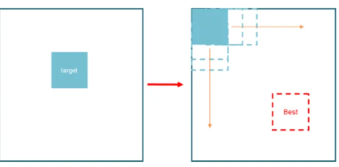
In the conventional texture-based tracking algorithm, the tracking process is doing with brute force way, like Fig 3.6. After user choose the texture region they are interested (ROI) at a timestep, the samples circled by ROI is set to be the target of the tracking process. These target samples are compared with all possible textures at the follow timestep and each of these samples should find a displacement. The numbers of the target samples and the size of the possible region dominate the numbers of comparisons tracking process needed, and affect the performance.
By deciding a tracking window of each target, we can reduce the comparisons and accelerate the tracking process (see Fig 3.7). But the numbers of the target samples is remain big if the dataset is large.
3.3 Hierarchical Feature Tracking 18
Figure 3.6: As we choose the target from left timestep, a brute force algorithm is apply until we find the best match.
Figure 3.7: As we choose a tracking window, we can reduce the comparisons we need. We use multi-resolution hierarchy, that has strongly spatial coherence and data distribution properties to reduce the target samples and estimate the tracking window of our target samples. In the tracking process, the user specify the area to track with ROI (region of interest) at timestep t. With precalculated hierarchical sampling, the ROI region contains lots of texture samples at each level of timestep t (see Fig 3.8). With the spatial coherence, we can take each sample point from level 0 of the data resolutions as one sample hierarchy. Each sample hierarchy refer to one independent tracking process. After the ROI is decided, the numbers of sample hierarchy is settled, and the target samples of each sample hierarchy are pushed into the tracking queue.
The multi-resolution feature tracking algorithm bas been used in many image processing and computer vision field. Here we extend to volume dataset with multi-resolution data hierarchy. For each sample hierarchy the ROI circled, we apply a two steps algorithm from root to leaves. First, at the root sample, as we don’t have the feature motion information, we use conventional brute force algorithm to find a best match of the root sample from next timestep t + 1. Second,
3.3 Hierarchical Feature Tracking 19
Figure 3.8: With wavelet transform, every parent node can be separate to 4 child node in 2D for every children sample node, we use the parent’s match result as a motion information, which help us to specify the tracking window’s location. Actually, if the match result is perfect, since every parent can separate to 4 child node in 2D, these children nodes should have the same perfect match with the same distribution. We can not ensure the result is perfect, so as our process moves down, we enlarge the area of the tracking window by one ring of the parent, that is one parent node will determine a size of six by six tracking window size in 2D, see Fig 3.9. Note that, if we analyze the tracking results of the root level for several timesteps, the tracking window for the root sample can be predict by the historical motion information.
With these steps, we can summarize the algorithm to Fig 3.10. Note that we take every texture sample comparison independently, the spatial coherence is ensured, but will not limits the flexibility of the data motions. Second, the parameter that controls the size of tracking window enlarging can affects by the speed of the data shifting. In our experiment, one ring is bigger enough for general dataset.
For each texture sample, the tracking process is independent, so we can have a flexible tracking result for general data evolution, such as creation, dissipation, bifurcation and amal-gamation, see Fig 3.11. For ”bifurcation”, as the feature involve several texture sample at the root level, when we apply tracking process for each texture sample, we will find that these sam-ple point move apart from each other. It refer to the same rules for ”amalgamation” operation when texture sample move close. For ”dissipation” operation, it can be done when we can not find a match within a acceptable threshold. The only problem come to the data operation of
3.3 Hierarchical Feature Tracking 20
Figure 3.9: Parent node can decide a 6x6 tracking window size.
”creation”. Since our works use the timestep t to track the timestep t + 1, it means that if the feature did not shown in the past, we will not have focuses on this particular feature. But, we have think of some possibly method to overcome this problem by backward tracking within the same dataset.
3.3.2
Feature Sample Comparison
After the tracking window of a texture sample point has been estimated, three distance mea-surement function is applied to find the ”best match”. the ”feature distance” function F D is defined as:
F D(Sti
xyz) = arg min{ maxx X p=minx maxy X q=miny maxz X r=minz [αT ED(Sti xyz, S ti+1 pqr )+ βP ED(Sti xyz, S ti+1 pqr ) + γF OS(S ti xyz, S ti+1 pqr )]} (3.6) T ED(Sti xyz, S ti+1 pqr ) = v u u t 39 X m=1 (T Fm(Sti) − T Fm(Sti+1))2 (3.7)
3.3 Hierarchical Feature Tracking 21
Figure 3.10: The tracking process of one texture sample hierarchy. P ED(Sti xyz, S ti+1 pqr ) = q (Pti x − P ti+1 p ) 2 + (Pti y − P ti+1 q ) 2 + (Pti z − P ti+1 r ) 2 (3.8) F OS(Sti
xyz, Spqrti+1) = (mean(Sxyzti ) − mean(Spqrti+1)) + (stdDev(Sxyzti ) − stdDev(Spqrti+1))) (3.9)
where Sti
xyz is the subvolume under consideration at time step i, (minx, miny, minz) and
(maxx, maxy, maxz) represent the estimated tracking window in which the feature could lie,
T ED(Sti
xyz, S ti+1
pqr ) is the 39-dimensional texture Euclidean distance function between the
fea-ture under consideration and the current location within the tracking window, T Fm is the filter
function to calculate the texture features, P ED(Sti
xyz, S ti+1
pqr ) is the feature displacement between
the target and the current location, Pti
xyzis the position of the sub-volume Sxyzti , F OS(Sxyzti , S ti+1
pqr )
is the first-order statistics distance between the target and the current location, includes mean and standard deviation. The α, β and γ is the weighted summation parameters of these three distance functions.
At the comparison step, a target sample point has been assigned one tracking window. For finding the ”best match” in the tracking windows, we have to compare the target with the whole
3.3 Hierarchical Feature Tracking 22
Figure 3.11: Conventional data motions.
range of the tracking window. For speed up the comparison process, we use the data maximal and minimal values to remove those unlikely points in the tracking window with two simple data range check. Next, we calculate the F D function for comparison scoring. We choose the sample points which has the minimal score as the most likely points in the tracking window, which we called ”match point”. Here, for result checking of the ”match point”, we have to ensure the ”match point’s” score is below some threshold ε. If we can not find a ”match point”, then the tracking process of this target point is fail, which refer to ”no match” or ”feature disappear”.
For simple rotational invariance of the feature tracking process,we rotate every sample point in the tracking window by ±45 degrees, and compare with the un-rotated target sample point. This means that if we find a point, which rotated for a little degree has the smallest value, we can assume the raw data had been rotated, see Fig 3.12. We can extend our BM function as:
F D(Sti
xyz) 0
= min
i,j,k∈{−45,0,45}F D(RS(i,j,k)) (3.10)
3.3 Hierarchical Feature Tracking 23
Figure 3.12: The figure on the left is the example drawing, which the yellow bar stand for the peak of the filter kernel. From top to down stand for the filter bank of a data in 2D, which has 4 different directions. In the comparison step, if we don’t have the rotational comparison, then we can find that target and the Sample A is totally different on every filtered value. On the other hand, we can find that target(1) has the similar value with Sample B(2), target(2) is similar to Sample B(3), and so on.
C H A P T E R
4
Result
All experiments are performed on Intel core 2 due E6750 2.66GHz PC using NVIDIA Geforce 8600 GT graphics hardware.
4.1
Example Data Sets
The time-varying data set used in our testing is Turbulent Vortex Simulation data set. This data set was provided to Kwan-Liu Ma by Dr. D. Silver at Rutgers University. Now this data set is made available at the TVDR data repository set up by a US NSF ITR project. The original data set store floating vorticity value at each grid point. There are 128 × 128 × 128 voxels, and a total of 100 time steps. For simplicity reason, we convert the floating variables into 16-bit integers. We take first 64 time steps as our test data set. (see Table 4.1)
Data set Resolution Time steps Size of each time step Total size Vortex 128x128x128 64 4 MB 256 MB
Table 4.1: The data set used in our testing.
4.2 Preprocessing Result 25
(a) (b)
Figure 4.1: The Vortex data set.
4.2
Preprocessing Result
For texture attributes computation, the Gabor filter bank is computed. We use sphere-shaped 3D Gaussian envelope, which has a constant σ = 5. The filter kernel size is set to be 8 × 8 × 8. The 3D frequencies of the complex sinusoid are choose to be 18, 38, and 68.
In Vortex dataset, we chose the block size to be 32 × 32 × 32, and this leads to a 3-level hierarchy octree with 73 rendering nodes. The texture samples are decided by uniform sampling with fifty percent overlap, and this lead to a 3-level hierarchy with 73 root samples, and totally 73+ 153+ 313 = 33509 texture samples. The require space to store preprocessing table is small,
and will not increase the disk overhead. (see Table 4.2)
Data set Root resolution Filter Size Root samples Num Data size Vortex 32x32x32 8x8x8 7x7x7 117 KB
4.3 Run Time Tracking Result 26
4.3
Run Time Tracking Result
Here we test several different ROI, to verify our algorithm’s correctness. For first test, the ROI chose 2 samples at the root level, and here we show several time frame with second level samples’ view. (see Fig 4.2)
(a) Time 0 (b) Time 1 (c) Time 6
(d) Time 12 (e) Time 18 (f) Time 24
Figure 4.2: Tracking result.
In Fig.4.2, the tracked samples are marked as colored spheres, and each sample is colored differently from red to blue. At frame 1, we can find that some samples are outside the ROI, it is because the parent of these samples are circled by the ROI (see Fig4.2(a)). Here, we find that ROI is not quit applicable for some dataset, which is not always cubic-like, and a sufficient user interface is needed. Except these outsider, we show that when the feature moves right, our group of samples can follow this movement. Frame 18 and 24 show that, when feature texture is too small, the information is not enough to let us track the feature. We can use some threshold
4.3 Run Time Tracking Result 27 ε to discard these unmatched samples. For Performance testing, the tracking time is determine by the numbers of comparisons needed. In this case, we have 2 root samples, and each of them will compare with 73 samples at the first tracking step. For each root samples, one-neighbor extension is applied and each of the eight children need 113comparisons. For 3-level hierarchy, totally 2 × 73+ 2 × 8 × 113+ 2 × 82× 113sample comparisons are needed, and it costs average
4.85(s). The equation can summarize as N3+(8×113)×(87 level−1). N is the numbers of samples at root level.
We also test the results using conventional brute force methods, see Fig 4.3. The user’s view is slightly different, but it shows that the tracking results are quite similar to our hierarchical method results. In this case, the numbers of comparisons needed are 313for each sample at the leave level, and it costs average 4.27(s). The equation can summarize as (2level× (N + 1) − 1)3.
N is the numbers of samples at root level.
(a) Time 0 (b) Time 1 (c) Time 6
(d) Time 12 (e) Time 18 (f) Time 24
4.3 Run Time Tracking Result 28 Compare the grows of comparisons of the brute force method and our hierarchical method, two circumstances are found. See Fig 4.4(a), when the numbers of root samples increase, the numbers of comparisons needed for brute force method raises quickly. In contrast, when the numbers of level increase, the numbers of comparisons needed for hierarchical method raises (see Fig 4.4(b)). Finally, we can draw these two equations together, the yellow surface is stand for brute force method, and the red one is hierarchical method. It shows that the brute force method get worse performance than the hierarchical tracking method, when the level and the samples increase. (Fig 4.5)
(a) Numbers of root samples increase
(b) Numbers of level increase
4.4 Discussion 29
(a) Numbers of root samples increase
Figure 4.5: The grows of comparisons for two different tracking algorithm.
4.4
Discussion
There are several subjects that we want to discuss about. First, the texture sampling rate and sampling criteria strongly affect the tracking algorithm. Increase the texture sampling rate can increase the correctness of samples’ displacement, but it also enlarge the pre-computed table sizes and increase the preprocessing times. When the data size of the texture attributes exceeds the memory size, we have to split the attributes to several data regions for storing. In this case, it may costs more disk I/O overheads at the tracking process. Importance sampling is a way to decrease false sampling, but the importance must be defined first.
Second subject is about finding match at the tracking step. In our algorithm, only one match is marked as tracking result. Actually, when we do sample comparisons, sometimes there are
4.4 Discussion 30 several samples that have similar attributes. When we choose different matching sample, the overall tracking result may change differently. These matching information can help choosing a tracking result with smaller global error. Still, global error of a tracking result is hard to define in feature tracking field. Without ground true, usually we can only judge a tracking result with human vision.
Third, the user interface and rendering issue. The cubic-like ROI is not feasible for any kinds of datasets, and a more efficiency way to choose the target samples is needed. Another, marking the tracking result may help user observe the sample displacements, but when the numbers of samples grow, it may cause ambiguities. This problem can solve by rendering the tracking path or other object-like rendering techniques.
C H A P T E R
5
Conclusion
In this chapter, we give brief summary of the thesis, and suggest some directions of future work.
5.1
Summary
In this thesis, we proposed a efficient texture-based feature extraction and tracking algorithm with multi-resolution hierarchy. In the preprocessing step, texture attributes are computed by Gabor filtering at each level of multi-resolution hierarchy. With spatial coherence, these at-tributes are builded as a texture sample hierarchy. In the run-time, a hierarchical feature tacking algorithm is applied. From root to leaves of the texture sample hierarchy, we use the parents tracking result to help children decide their tracking window. We demonstrate how this struc-ture can perform more efficient tracking in texstruc-ture-based datasets. The tracking algorithm is also adapted with multi-target feature.
5.2 Future Work 32 The contributions of our work can be summarized as :
• We proposed a hierarchical feature tracking algorithm, which – Speed up the texture-based feature tracking processes. – Spatial coherence is guaranteed.
– The information of the region probability is easily obtained within the tracking processes.
5.2
Future Work
In the scientific research, there are different applications for observing dataset. With texture-based method we proposed, the feature’s movements are followed, but with the idea of tex-ture sample comparison, featex-tures can be separated to several textex-ture sample points that hard to maintain other application, such as object picking, feature isolation. The feature is defined as a small local area texture in our works. Features user specified with ROI contain thousands of pre-computed texture sample points, and with independent texture-based feature tracking algo-rithm, the connectivity of these sample points are hard to maintain after we track the feature. We address several methods to overcome this problem by combines our method with object-based feature extraction techniques. In the following sections, first we will introduce object-based feature extraction algorithm, and then three different approaches are discussed with different applications.
5.2 Future Work 33
5.2.1
Object-based Feature Extraction
The region growing algorithm works by doing a breadth-first search(BFS) on voxels starting from a seed voxel or set of voxels [13]. Like any BFS algorithm, this is done with a queue of voxels to visit. This queue is pried with the seed voxels(s) then each voxel in the queue is tested to see if it belongs to the region. If it is, then it is marked as being part of the region. Then, any of its neighbors that have not yet been visited are enqueued. This process is repeated until the queue is empty, at which point every voxel in the region has been visited. The region growing algorithm is very flexible, since the test to see whether a voxel should be in the region or not can be based on several different properties, such as a threshold value or gradient magnitude. For our purposes, a threshold value can be used.
In our works, the threshold and the searching seed can be set base on our feature tracking result. Since the texture-based tracking results represent the most possibly locations of the feature positions. We can use these positions and there texture properties to estimated the region growing parameters.
With lots of sample points as our tracking result, first we have to cluster these points to several groups in the manner of their locations. Several clustering algorithms are proposed in image segmentation and pattern recognition field, such as K-means algorithm. After we clustered these points, texture properties, such as mean, standard deviation of the points in each groups can be used to estimate the threshold value of the region growing process independently by histogram statistics. The histogram help us to measure the data distribution of the texture in one group. For continue data, a normal distribution is a fine guess to determine the object boundary. Finally, the result of the region growing process can be used for other applications, such as, object picking and feature isolation.
5.2 Future Work 34
5.2.2
Hybrid Method Approach
Texture-based Tracking with Object Extraction Process (Fig 5.1)
In this approach, we take object-based extraction as an bonus for feature isolation and picking. First, we use a standard texture-based feature tracking algorithm we proposed, and then use the results to help extracting the feature object. In figure 5.1, after our texture-based tracking process done, we use a clustering algorithm to find groups of these texture feature samples. Histogram statistics of the samples in the same groups are builded with samples data. With mean and standard deviation, we choose a data region to estimate the threshold of the region growing processes we need. Finally, the region growing process can help us extract the object liked features. This approach is for data which user have already had a thought of what they want, and with tracking the movement and object extracting process, user can isolate the feature for observations.
Figure 5.1: Hybrid method which texture-based tracking result as an object extraction process input.
5.2 Future Work 35 Object-based Extraction with Texture-based Correspondence Test (Fig 5.2)
In the previous object-based feature extraction and tracking algorithm, the features for each timestep are extracted separately and then the system will try to associate them through time. Many of the original algorithms correspond feature based on whether or not their regions over-lap in adjacent timesteps [28] [29]. For breaking the limits of features overover-lapping, we can use texture-based comparison to help finding the correspondences. The texture properties are cal-culated after object extracting processes in each timestep, and the texture comparison process can use to measure the object’s similarity. For each timestep, every feature object will contain several texture samples. Several samples distribution properties can be considered, such as most of the samples must find correspondences in one feature object to ensure this feature object is the correct tracking result. This approach is for object like dataset, and several object-based feature extraction techniques and applications for tracking result can be used.
Figure 5.2: Hybrid method which object-based extraction with texture-based correspondence test.
5.2 Future Work 36 Texture-based Tracking with Motion Pattern Recognition (Fig 5.3)
Since the tracking process of each texture samples hierarchy is independent in our works, the samples’ motion information can be extracted. First, every texture samples in the coarse reso-lution are tracked by our method, then the displacement information can help us tracking the feature by observing the samples relations. This method do not need the user input and the extraction and tracking process can be done in pre-processing time.
Bibliography
[1] S. Belongie, C. Carson, H. Greenspan, and J. Malik. Color- and texture-based image segmentation using em and its application to content-based image retrieval. In ICCV ’98: Proceedings of the Sixth International Conference on Computer Vision, pages 675–682, Washington, DC, USA, 1998. IEEE Computer Society.
[2] J. Bigun. Speed, frequency, and orientation tuned 3-d gabor filter banks and their design. ICPR ’94: Proceedings of the International Conference on Pattern Recognition, c:184– 187, Oct 1994.
[3] I. Boada, I. Navazo, and R. Scopigno. Multi-resolution volume visualization with a texture-based octree. The Visual Computer, 17(3):185–197, 2001.
[4] R. Botchen, M. Chen, D. Weiskopf, and T. Ertl. Gpu-assisted multi-field video volume visualization. In IWVG’06: Proceedings of the Fifth International Workshop on Volume Graphics ’06, pages 47–54, Boston Park Plaza, Boston, Massachusetts, USA, July 2006. [5] J. Caban, A. Joshi, and P. Rheingans. Texture-based feature tracking for effective
time-varying data visualization. Visualization and Computer Graphics, IEEE Transactions on, 13(6):1472–1479, 2007.
[6] M. Fernandez, A. Mavilio, and M. Tejera. Texture segmentation of a 3d seismic section with wavelet transform and gabor filters. In ICPR ’00: Proceedings of the International
Bibliography 38 Conference on Pattern Recognition, page 3358, Washington, DC, USA, 2000. IEEE Com-puter Society.
[7] D. Gabor. Theory of communication. In Proceeding of the Institute of Electrical Engi-neers, volume 93, pages 429–457, 1946.
[8] B. Galvin, B. McCane, and K. Novins. Robust feature tracking. In DICTA ’99: Proceed-ings of the Fifth International Conference on Digital Image Computing, Techniques, and Applications ’99, Perth, Australia, December 1999.
[9] X. Guan, G. Pan, and Z. Wu. Automatic categorization of traditional chinese painting images with statistical gabor feature and color feature. In In Lectures in Computer Science, pages 743–750. Springer Berlin/Heidelberg, 2005.
[10] B. Guo. Interval set: A volume rendering technique generalizing isosurface extraction. In VIS ’95: Proceedings of the 6th conference on Visualization ’95, page 3, Washington, DC, USA, 1995. IEEE Computer Society.
[11] S. Guthe, M. Wand, J. Gonser, and W. Straßer. Interactive rendering of large volume data sets. In VIS ’02: Proceedings of the conference on Visualization ’02, pages 53–60, Washington, DC, USA, 2002. IEEE Computer Society.
[12] G. Heidemann and H. Ritter. A neural 3-d object recognition architecture using optimized gabor filters. ICPR ’96: Proceedings of the International Conference on Pattern Recogni-tion, 4:70, 1996.
[13] R. Huang and K. Ma. Rgvis: Region growing based techniques for volume visualiza-tion. In PG ’03: Proceedings of the 11th Pacific Conference on Computer Graphics and Applications, page 355, Washington, DC, USA, 2003. IEEE Computer Society.
[14] F. V. Hundelshausen and R. Rojas. Tracking regions and edges by shrinking and growing. In Proceedings of the RoboCup ’03 International Symposium, Padova, Italy, 2003.
Bibliography 39 [15] G. Ji, H. Shen, and R. Wenger. Volume tracking using higher dimensional isosurfacing. In VIS ’03: Proceedings of the 14th IEEE Visualization ’03, page 28, Washington, DC, USA, 2003. IEEE Computer Society.
[16] C. Ko, H. Liao, T. Wang, K. Fu, C. Lin, and J. Chuang. Visualization of large time-varying volume data using multi-resolution technique with video based compression. In Computer Graphics Workshop ’07, 2007.
[17] E. LaMar, B. Hamann, and K. Joy. Multiresolution techniques for interactive texture-based volume visualization. In VIS ’99: Proceedings of the conference on Visualization ’99, pages 355–361, Los Alamitos, CA, USA, 1999. IEEE Computer Society Press. [18] P. Ljung, C. Lundstrom, A. Ynnerman, and K. Museth. Transfer function based adaptive
decompression for volume rendering of large medical data sets. In VV ’04: Proceed-ings of the 2004 IEEE Symposium on Volume Visualization and Graphics, pages 25–32, Washington, DC, USA, 2004. IEEE Computer Society.
[19] A. Madabhushi, M. Feldman, D. Metaxas, D. Chute, and J. Tomaszewski. A novel stochas-tic combination of 3d texture features for automated segmentation of prostastochas-tic adenocar-cinoma from high resolution mri. Medical Image Computing and Computer-Assisted In-tervention, 2:581–591, 2003.
[20] D. Pinskiy, E. Brugger, H. Childs, and B. Hamann. An octree-based multi-resolution approach supporting interactive rendering of very large volume data sets. In Proceedings of the International Conference on Imaging Science, Systems, and Technology, pages 16– 22, 2001.
[21] J. Plate, M. Tirtasana, R. Carmona, and B. Fr¨ohlich. Octreemizer: a hierarchical approach for interactive roaming through very large volumes. In VISSYM ’02: Proceedings of the symposium on Data Visualisation ’02, pages 53–ff, Aire-la-Ville, Switzerland, Switzer-land, 2002. Eurographics Association.
Bibliography 40 [22] F. Post, B. Vrolijk, H. Hauser, R. Laramee, and H. Doleisch. The state of the art in flow
visualization: Feature extraction and tracking. Eurographics, 22(4):775–792, 2003. [23] Z. Qian, D. Metaxas, and L. Axel. Extraction and tracking of mri tagging sheets using a
3d gabor filter bank. Engineering in Medicine and Biology Society, 2006. EMBS ’06. 28th Annual International Conference of the IEEE, pages 711–714, 2006.
[24] F. Reinders, F. Post, and H. Spoelder. Attribute-based feature tracking. In Data Visualiza-tion 99, pages 63–72. Springer Verlag, 1999.
[25] R. Samtaney, D. Silver, N. Zabusky, and J. Cao. Visualizing features and tracking their evolution. Computer, 27(7):20–27, 1994.
[26] H. Shen, L. Chiang, and K. Ma. A fast volume rendering algorithm for time-varying fields using a time-space partitioning (tsp) tree. In VIS ’99: Proceedings of the conference on Visualization ’99, pages 371–377, Los Alamitos, CA, USA, 1999. IEEE Computer Society Press.
[27] D. Silver. Object-oriented visualization. IEEE Comput. Graph. Appl., 15(3):54–62, 1995. [28] D. Silver and X. Wang. Volume tracking. In VIS ’96: Proceedings of the 7th conference on Visualization ’96, pages 157–ff, Los Alamitos, CA, USA, 1996. IEEE Computer Society Press.
[29] D. Silver and X. Wang. Tracking scalar features in unstructured datasets. In VIS ’98: Proceedings of the conference on Visualization ’98, pages 79–86, Los Alamitos, CA, USA, 1998. IEEE Computer Society Press.
[30] S. Smith and J. Brady. Asset-2: real-time motion segmentation and shape tracking. Trans-actions of the IEEE on Pattern Matching and Machine Intelligence, 17(8):814–820, Jun 1995.
Bibliography 41 [31] F. Tzeng and K. Ma. Intelligent feature extraction and tracking for visualizing large-scale 4d flow simulations. In SC ’05: Proceedings of the 2005 ACM/IEEE conference on Supercomputing, page 6, Washington, DC, USA, 2005. IEEE Computer Society.
[32] C. Wang and H. Shen. A framework for rendering large time-varying data using wavelet-based time-space partitioning(wtsp) tree. Technical Repost OSU-CISRC-1/04-TR05, Jan-uary 2004.
[33] C. Wang and H. Shen. Lod map - a visual interface for navigating multiresolution volume visualization. IEEE Transactions on Visualization and Computer Graphics, 12(5):1029– 1036, 2006.
[34] C. Wang, A. Garcia, and H. Shen. Interactive level-of-detail selection using image-based quality metric for large volume visualization. IEEE Transactions on Visualization and Computer Graphics, 13(1):122–134, 2007.
[35] J. Wang, T. Xu, H. Shum, and M. Cohen. Video tooing. In Proceedings of ACM SIG-GRAPH ’04, pages 574–583, 2004.
[36] M. Weiler, R. Westermann, C. Hansen, K. Zimmermann, and T. Ertl. Level-of-detail volume rendering via 3d textures. In VVS ’00: Proceedings of the 2000 IEEE symposium on Volume visualization, pages 7–13, New York, NY, USA, 2000. ACM.
[37] T. P. Weldon and W. E. Higgins. An algorithm for designing multiple gabor filters for segmenting multi-textured images. In In Proc. IEEE Intl. Conf. Image Proc, pages 4–7, 1998.
[38] T. Xu, M. Sonka, G. McLennan, J. Guo, and E. Hoffman. Mdct-based 3-d texture clas-sification of emphysema and early smoking related lung pathologies. MedImg, 25(4): 464–475, April 2006.