CHINESE JOURNAL OF PHYSICS VOL. 2, NO. 2 OCTOBER, 1964
Angular Momentum Distributions in the Atomic Nuclei
JE N N- LIN HWANG ($r.#& & )
Department of Physics,- National Taiwan University, Taipei, Taiwan
AND
JY I- CH E R N G HORNG (02 8 &)
Tatung In&tie of Technology, C?uuzg-Shari Northern Road, Taipei, Taiwan
(Received June 15, 1964)
The problem of how many protons (neutrons) of a given orbital angular mo-m e n t u mo-m Itr are to be found in a nucleus of a given proton numo-mber Z (neutron number N) is reinvestigated by means of the improved Thomas-Fermi method.
Three kinds of nuclear models are calculated: The types of potentials chosen arc (i) square well potential, (ii)-the Green’s potential, and (iii) the Green’s potential plus 45 times the Thomas-Frenkel spin orbit term. The parameters involved in the potentials are adopted from the paper of Hwang and Yang, which may exactly re-produce the nuclear radii, trends of binding energies, and location of 3s and 4s maxima in the neutron scattering cross section. The eigenvalues calculated by Green are used to simplify the procedure of calculation. The results are then compared with the empirical data compiled by Klinkenbeig. For the last type of potential, the calculation is almost perfectly exact. T h e first appearance of particles of the next higher angular momentum is almost exact for each model. The puzzle in the Yang’s treatment of the first appearance problem is then solved. The crigin of the appearance of magic numbers in the Yang’s calculation is explained in the light of the present theory.
ANGULAR MOMENTUM DISTRIBUTIONS
T
HE number of neutrons (or protons) z1 with a given angular momentum Iiz in the atomic nuclei is determined by means of the improved Thomas-Fermi method”. Three kinds of nuclear models withand
(9
(ii)
(iii)
the square well potential
V( 7-) = - v, f o r r-da,
V(r)=0 f o r r>a,
the Green’s potential
V(r) = - v, f o r rLa, V(r) = - V,exp[ - (r -a)jd] for r>a, the Green’s potential plus 4.5 times the Thomas-Frenkel spin orbit term
are investigated. The eigenvalues of the Schrddinger equation with these potentials have been calculated and illustrated in diagrams by Green2). These eigenvalues serve
1) J. L. Hwang, Chin. J . Phys. 1, 7 4 (1963) and 2, 28 (1964) 2) A. E. S. Green and K. Lee, Phys. Rev. 99, 772 (1955)
A. E. S. Green, Phys. Rev. 102, 1325 (1956) A. E. S. Green, Phys. Rev. 104, 1617 (1956).
80
1- L -_,
--ANGULAR MOMENTUM DISTRIBUTION 81
us the first guess f o r d e t e r m i n i n g t h e m a x i m u m e n e r g y (El)mar involved in the expression’)
n
I
=
x21+ 1)
2h i
SC
2m ((E,),,,- V(r)) -‘“WI” &+$}.
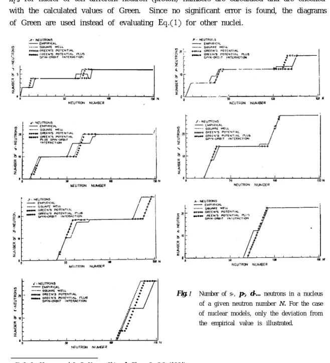
The parameters V,, a, and d involved in the potentials are adopted from the paper of Hwang and Yang3), which may exactly reproduce the nuclear radii, trends of binding energies, and location of 3s and 4s maxima in the neutron scattering cross section. n,‘s for nuclei of ten different neutron (proton) numbers are calculated and are checked with the calculated values of Green. Since no significant error is found, the diagrams of Green are used instead of evaluating Eq.(l) for other nuclei.
Fig. I Number of s-, p-, d-... neutrons in a nucleus of a given neutron number N. For the case of nuclear models, only the deviation from the empirical value is illustrated.
82 J. L. HWANG AND J. C. HORNG
S - PROTONS - EMPIRICAL z”
--- SQUARE WELL ooD00 GREEN’S POTEN TI A L
I= ,ODH. GREEN’S POTENTIAL PLUG u” SPIN-ORBIT INTERACTION a
(b, , , , ,
7-y
50 IW 2 PROTON NUMBER 2m? E -a _ 4 -& IOz
5
-2
O-0 d- PROTONS - EMPIRICAL - - - - S Q U A R E W E L L PROTON N U M B E R 9 - PROTONS - EMPIRICAL --- SQVARE W E L Lz” ooooo GREEN’S POTENTIAL
e . . . GREEN’S POTENTIAL z a PROTON NUMBE’R P- PROTONS - EMPIRICAL 2 L --- SQUARE WELL
oooa, GREENS POTENTIAL
.e.w GREEN’S POTENTIAL RUS S P I N - O R B I T INTERACT,ON
PROTON N U M B E R
f-
PROTONS- EMPIRICAL --- SQUARE W E L L OWOO GREEN’S POTENTIAL . . . GREEN’S POTENTIAL PWS SPIN-ORBIT INTERACTION 01 ’ J ’ ’ 1 1 ( * 8 0 50 11 PROTON N U M B E R h - PROTONS - - E M P I R I C A L _ _____ SQUARE WELL o- GREENS POTENTIAL 0 50 10 PROTON NUMBER
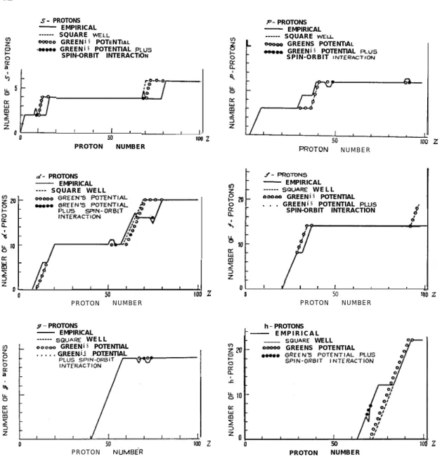
Fig. 2 Number of S-, p-, d-... protons in a nucleus of a given proton number Z. For case of nuclear models, only the deviation from the empirical valus is illustrated.
The results are illustrated in Figs. l-4. The empirical curves determined from the paper of Klinkenberg4) are also given there. Since the conformity between the calculated and empirical values is very good, only deviations form the empirical values are illustrated. For the last type of potential, the conformity is almost complete. The first remarkable evidence revealed by Figs. 1-2 is that the difference between the square well potential and Green potential is small. The second is that the first appearance of the next higher angular momentum is not so different from the exact values. T h i s is a result of our correct choice for the potential parameters.
ANGULAR MOMENTUM DSTRIBUTIONI THE FIRST APPEARANCE PROBLEM
83
In the early stage of the theory of nuclear shell structure, Yang51 was guided by a principle that the successive appearance of particles of higher angular momentum is associated with the successive beginning of new shells, and found that the first ap-pearance of neutrons (protons) with angular momentum states s, p, d, f.o.occurs re-spectively at the nuclei of neutron (proton) number 1, 3, 9, 21, 29, 51 83...(magic number plus one). From the empirical data or the former calculation Figs. l-2 it is, however, seen that the first appearance of these nucleons would occur at 1, 3, 9, 21, 41, 71, 113..., if the magnitude of spin-orbit coupling were suitably chosen. The truth of Yang’s discovery is thus now denied. However, it seems that the origin of this interesting accident, the appearance of magic numbers, remains still unclarified.
The equation for the number of particles with the angular momentum Iii employed by him was
?Q=-; (I+ +)s (P”(r) - (Z++)W/+* dr,
which has just the same form as. Eq.(l) used by us except for lacking the last term (2Z+ 1). This last term is the key of the problem. In our distibution curves (Figs. l-2), if shifting the abscissa ul;w-ard by (2Z+ 1) + 1 units, that is, if raising two units for s-state, four units for p-state, six units for d-state and so on, it can readily be seen that the s-, p-, d-,-.- neutrons (protons) appear firstly at N (or 2) = 3, 7, 15, 29, 51, 83, 127.... Apart frcm the first three numbers, they all reprcduce the Yang’s discovery.
This may more precisely be stated with the Ievel schemef). In the pIace where a higher angular mcmentum I appears for the first time, the splitting of the Z-state level into two levels with j=Z+ + and j=Z-+ is particularly large, and the higher magic number will occur there. On the other hand, the level with j=Z++ is lower t h a n the level with j-Z--&, and therefore the particles, 2(1+-J-)+ 1=2Z+ 2 in number, occupying the lower level precede to appear in the distribution curve. When the ab-scissa is raised, these 21+2 particles sink and the upper edge of the lower major shell becomes a sign of the first appearance of Z-state (j=Z-+) particles. The occurrence of the magic number is thus explained. As to the first three magic numbers, Yang attributed them to a modification of nuclear shaFe, that is, he assumed that for light nuclei the nuclear density shrinks to a gaussian form.
This work was supported by the National Council on Science Development.
4) 5) 6)
P. F. A. Klinkenerg Revs. Modern Phys. 24, 63 (1952)
L. M. Yang, Proc. Phys. Etc. (Lcndon) 64, 632 (1951); M. Earn and L. Yang, Nature 166, 339 (1950) See for example, M.G. Mayer ar.d J.H.D. Jensen, Elcmcntaty Tkoly of &clear Shell Structute ( J o h n Wiley and Sons, Inc., New York, 1955) p. 58