Comments on “A linear solution to the kinematic parameteridentification of robot manipulator” and some modifications

IEBE TRANSACTIONS ON ROBOTICS AND AUTOMATION, VOL. 11, NO. 5, OCTOBER 1995 777

Correspondence

Comments on "A Linear Solution to the

Kinematic Parameter Identification of Robot

Manipulator" and Some Modifications

Sheng-Wen Shih, Yi-Ping Hung, and Wei-Song Lin

Abstract-The paper by Zhnang and Roth [5] presents a Linear solution to kinematic parameter identification of robot manipulators. With their method, the orientation parameters for all revolute joints have to be solved first before solving for the translation parameters for all revolute joints and the orientation parameters for all prismatic joints simultaneously. Our major modification here is to decompose the kinematic parameters estimation problem into many subproblems of a single joint axis such that the complexity is reduced and easier implementation is derived. In addition, this gives a unified solution for any serial manipulator with an arbitrary combination of prismatic and revolute joints.

I. INTRODUCTION

Zhuang and Roth [5] proposed a linear method for the identification of unknown kinematic parameters of robot manipulators from end- effector pose measurement and robot joint position readings at some configurations. Their work is of great value for many applications. While their calibration method was clearly illustrated with the use of an all-revolute robot, a Cartesian robot, and a Stanford-arm-type robot, no general procedure was given for dealing with an arbitrary type of robot. In the derivation of their linear solution, the rotation matrix and translation vector were considered separately. When solving for the translation vectors, the translation vectors of all joints have to be solved simultaneously, which makes implementation very complicated, e.g., [5, eq. (16), (19)]. Moreover, if a robot contains some prismatic joints, then the directions of the prismatic joint axes have to be solved together with the translation vectors, e.g., [5, eq. (ZO)], and some nonlinear constraints should be involved to force the direction vectors to be unit vectors. However, these constraints were not discussed in [5].

We shall show that, due to the good structure of the complete and parametrically continuous (CPC) kinematic model [4], the kinematic parameter identification problem can be decomposed into many kine- matic parameter calibration subproblems for each individual prismatic or revolute joint. With this kind of decomposition, the calibration procedure can be applied to any serial manipulator composed of prismatic and revolute joints. Since the scale of the problem is reduced to that of single joint, we can derive the exact closed-form solution of the direction of the prismatic joint axis estimation, even with the nonlinear constraint. Also, the calibration method can be implemented in an easier way. Although the calibration problem is

Manuscript received June 3, 1994; revised December 29, 1994. This work was supported in part by the National Science Council, Taiwan, ROC, under

S.-W. Shih and W . 3 . Lin are with the Institute of Electrical Engineering, Y.-P. Hung is with the Institute of Information Science, Academia Sinica, IEEE Log Number 941 1922.

Grant NSC-83-0408-E-001-0.

National Taiwan University, Taipei, Taiwan. Taipei, Taiwan.

decomposed into subproblems of a single joint, this does not mean that only that joint can be moved during the calibration procedure. In fact, for the calibration of a certain joint, our modified method can move all the calibrated joints, as can the original method of Zhuang and Roth [5].

11. PROBLEM FORMULATION

The CPC kinematic model for a revolute or prismatic joint is as follows (refer to [4]):

where

qi is the ith joint value,

(4)

and

L

o

0

o

i J

Notice that the CPC convention requires that any two consecutive joint axes have a nonnegative inner product, i.e., b z ,

2

0. In general, this requirement can be achieved by changing the sign of one of the joint values of consecutive joints. This is because changing the sign of the joint value is equivalent to reversing the joint axis for both revolute and prismatic joints. Therefore, we have slightly modified the convention of the CPC model by including a sign parameter, s I , as shown in (3).

Suppose we have a robot with n joints. Its world-to-end-effector transformation matrix can be expressed as

"Tn

= "To

...

( n - l ) T n . ₍₆₎

Without loss of generality, we assume that the kinematic parameters of the joints from the end-effector to the ( i

+

1)st joint are known, and that the unknowns to be estimated are the world-to-base transfor- mation, "To, and the kinematic parameters of joints 1,

. . .

,

i. Also, we assume that the world-to-end-effector transformation matrix can be measured. The same as in the calibration procedure described in Zhuang and Roth [5], when calibrating the ith joint, only those joints with known kinematic parameters plus the ith joint itself are permitted to be moved. By moving those joints (from the end- effector to the ith joint) to two different configurations and recording their corresponding world-to-end-effector transformation matrices, we have

(7)

1042-296X/95$04.00 0 1995 IEEE

118 IEEE TRANS

where "Tn1 and "Tn2 are the measured world-to-end-effector

transformation matrices, ('+l)lTnl and ('+l)'Tn2 can be computed

from the kinematic model since their kinematic parameters are known already. Instead of separating (6) into two parts, the rotation matrix equation and translation vector equation, as is the method used in [5] and [2], we decompose the problem into many kinematic parameter estimation subproblems of a single joint axis, before separating the rotation matrix part from the translation vector part.

By multiplying "TR; and "Ti; on both sides of (7) and (8),

respectively, we have the following equality:

Rearranging (9), we have

AQV, = V , A T (10)

where AQ E

QG1Qz2,

A T E ( ~ + ~ ) ~ T n l "T-'"T n l n 2 (z+1)2T-1 n 2 7

and V, is the unknown homogeneous transformation matrix to be estimated.

Notice that (10) can be separated into two equations: one is the rotation matrix equation and another is the translation vector equation, i.e., RAQ Rv, = Rv, RAT Rag t v ,

+

t A Q = RV, t A T

+

tV, (11) (12) and where

RAQ,

RAT, Rv,, R,, and Rot,(P,) are 3 x 3 rotation matrices of

AQ, AT,

v,,

R,, and Rot,(p,), respectively, and t a g , tal-, and

t v , are 3 x 1 translation vector of AQ, AT, and V , , respectively. In the following sections, we shall show how to solve the kinematic parameters of the prismatic and revolute joints from the above equations.

111. CALIBRATION OF A PRISMATIC JOINT

From (2), AQ = Trans([O 0 AqlT), or more specifically,

RAQ = 1 s X 3 and tag = [O 0 AqIT. By substituting RAQ and

t A Q into (12), we have

t A Q = Rv,tAT. (15)

Substituting (13) into (15), we have T

Rt t A Q = t A T

where

AT

E RotL(Pt)tAT, and

Pt

is the given redundant pa- rameters. Note that in the above equation, t A Q =

[o

0 AqIT;

therefore,

bLAq =

AT

(16)

where b: = [ - b , , , - b z , b e ,

.IT

is the third column vector of the rotation matrix RT.

Suppose we have M observations, i.e., Aq, and AT,, j =

1, 2,

. . . ,

M. We can solve b: by minimizing the following error using the least square method:

lACnONS ON ROBOTICS AND AUTOMATION, VOL. 11, NO. 5, OCTOBER 1995

where b'T b: = 1. The optimal solution to the above equation can be found to be [3]

By intuition, if the difference of the joint values, i.e., Aq3 (or equivalently, the length of

i , ~ , ) ,

can be made larger, then the S/N ratio will be larger, too. Therefore, a larger difference of the joint values would lead to more accurate results. Notice that if the third component of b: is negative, in order to be consistent with the CPC convention, we should change the sign of b: and let

s , = -1; otherwise, let s1 = +l. Once the unit vector b: is obtained, the rotation matrix, R,, can be computed with (5). Then, we can transform the redundant translation vector (refer to [3] for details),

t v , , into the CPC parameter format, i.e.,

IV. CAJBRATION OF A REVOLUTUION

JOINT

Note that for a revolute joint, AQ = Rot,(Aq), i.e.,

and

Substituting (19) and (20) into (11) and (12), we have

Rot,(Aq)Rv, = RV,RAT (21)

Rot, (Aq)tv, = Rv,tAT

+

t v ,

.

(22) and

By taking the transpose of both sides of (21) and then multiplying the unit vector, z = [0 1IT on the right, we have (by noticing that Rot,(-Aq)z = z), 0 (23) T T R$,z = RATRv,z. By use of (13), we have b: = Db: (24)

where b: is the same vector as in (16), and D Rot,(P,)R~TRotl(-P,). Since in (24), D is a rotation matrix, b: can be found, up to its sign, by computing the rotation axis of D

with the following method. The correct sign of b: can be determined such that the third component of b: is nonnegative.

Suppose we have M observations. Then, we have the following homogeneous equation

[

1:::::3]

b:

=

E b : = E z 0

where E is the error vector induced by the observation noise. The parameter vector b: can be estimated by minimizing

1 1 ~ 1 1 '

subject to IlbiII' = 1.. It can be shown that the solution for b: is the unit eigenvector of

The sign parameter, szr can be determined as follows. From (5),

we can compute R, from b l . Substituting the estimated Rt into (21), we have

R o t , ( s z . A d ) = Rv,RATR$,

E corresponding to the smallest eigenvalue.

IEEE TRANSACTIONS ON ROBOTICS AND AUTOMATION, VOL. 11, NO. 5, OCIDBER 1995 179

and the sign parameter, s ; , can be obtained from the following equation:

M

Notice that in order to estimate b: more accurately, the difference of the joint angle, i.e., Aq should be made larger. Otherwise, the

D matrix in (%), will approach a unit matrix when Aq is very small, which will cause the estimation of the rotation axis to be very sensitive to noise.

After b: is obtained, we can compute the rotation matrix R, and then post-multiply it by Rot,

(pl)

to obtain R v , . Next, by substituting R v , into (22) and rearranging it, we have [by noting that the third component of tv, is redundant (refer to [3] for details)]

cos (Aq)

-

1 - sin(Aq)

''I = Rv,tAT (25)

sin(Aq) cos(&) - 11

[it,.]

where t , , and t t , are the first two entries of tv,, and Rv, is a 2 x 3 matrix obtained by deleting the third row of R v , . The determinant of the 2 x 2 matrix on the left hand side of (25) is [2 - 2 cos (Aq)]. Therefore, (25) has a unique solution if and only if Aq

#

0. This

condition for uniqueness is always satisfied since we always move the joint being calibrated in the kinematic identification process. Again, we observe that a larger value of

Aq

will improve the robustness for the estimation of the kinematic parameters. Of course, if more than one observations are available, we can use the least square method to solve the two unknown translation components.

After all the unknown parameters are obtained, we can transform the translation vector, t v , , into the

CPC

parameter format by using (18). If it is necessary to let l , , = 0, then the following equation can be used to determine the redundant translation parameter, i.e., the third entry of t v , :

t t , *

=

- ( b * , z t q z

+

b Z , & , V ) / b 2 , *

providing that b t , is not equal to zero.

v.

DETF~FMNATION OF THE

WORLD-TO-BASE TRANSFORMATION MATRIX

After all the revolute and prismatic joints are calibrated, we can compute the world-to-base transformation matrix, "TO, defined in

(6). Suppose we have M observations, i.e., j = 1, 2,

... ,

M. By separating (6) into the rotation matrix equation and translation vector equation, we have R,, ="Ro0Rn3 (26) W and t,, = W R ~ o t n 3

+

wto (27) W

where

OR,,

and O t n 3 are, respectively, the 3 x 3 rotation matrix and

the 3 x 1 translation vector of the transformation matrix, OT,,

' 2 ' 1

, 1 3 T 2 ,

...

( n - 1 ) 3 T n 3 . From (26), we have the following

matrix equation:

A = " R O B

where A E ["R,1

...

"Rn,

. . .

"R,M] and B s

...

ORn3

.

.

.

'R,M]. By solving the following "rotation of subspaces" problem [l], minimize I ( A ~ - B~ " R F I I F subject to wR: "Ro = 1 3 3 0.450

,

1

-

0.400 E .E 0.350 6 0.250

:z

8

0.200

'=

0.150

g

0.300 0

f

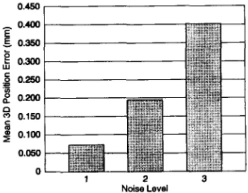
0.100 0.050 0 1 2 3 Ndse Level

Fig. 1. The mean 3-D position error against different noise levels.

we have the following procedure for finding the closed-form solution for "Ro:

1) Compute the matrix

c

s B A ~ .

2) Compute the singular value decomposition C =

USVT.

3) Compute "Ro = V U T .

After the rotation matrix, "Ro, is obtained, by substituting "Ro into (27), we have

M

w_{to = jj} 1 _{C ( w t n 3}

- "Rootn3)

3 = 1

which completes the calibration procedure.

VI. SIMULATION

To test our modified method for kinematic parameter identification, we ran a simulation for a six-revolute-joint Kawasaki Js-10 robot arm. In order to model robot pose measurement noise, we added three independent angular random noises having uniform distribution U [ - @ , 01 and three independent translational random noises having uniform distribution U[--7, 71, respectively, to the Z-Y-Z Euler

angles and the positions of the tool. Totally, 42 pose measurements, seven for each joint, were used for the calibration. The estimated kinematic parameters were tested by using 32 poses. Fig. 1 shows the mean 3-D position error against three noise levels, where in noise level 1, 0 = 0.01" and -7 = 0.1 millimeter, in noise level

2, 0 = 0.05" and -7 = 0.1 millimeter, and in noise level 3,

0 = 0.05" and T = 0.5 millimeter. These three levels of noise were

used in Zhuang and Roth's simulations [ 5 ] . This simulation showed that the position error was proportional to both the orientation and translational error. Therefore, to estimate the kinematic parameters accurately, an accurate pose measurement device is needed.

VII. SUMh,iARY

In this paper, we have shown that the kinematic parameter identi- fication problem can be decomposed into many kinematic parameter calibration problems of individual prismatic or revolute joints.

This

not only reduces the complexity of the identification problem, but also provides a calibration method that is general enough for any serial manipulator composed of prismatic andor revolute joints. By decomposing the problem, the closed-form solution for the direction of a prismatic joint axis is more accurate, mainly because a nonlinear unit vector constraint is included. It also provides intuition for reducing the estimation error by choosing larger magnitude of the difference of the joint values when constructing the calibration equations. This method has been tested by computer simulation, which shows that if the measurements of the world-to-end-effector

780 IEEE TRANSACTIONS ON ROBOTICS AND AUTOMATION, VOL. 11, NO. 5, OCTOBER 1995

transformation matrices are accurate, the calibration results can

also be very accurate. Although the kinematic parameters may not be parametrically continuous when the two consecutive joints are perpendicular to each other, this will not cause any problem if

[2] S. W. Shih, Y. P. Hung, and W. S. Lin, “Kinematic calibration of a binocular head using stereo vision with the complete and parametrically continuous model,” in Proc. SPIE Con$ Intell. Robots Comput. Vision

XI: Algorithms, Technol. Active Wsion, Nov. 1992, pp. 643-657.

fication of robot manipulator,” Tech. Rep. TR-94-004, Inst. of Inform. Sci., Academia Sinica, Nankang, Taipei, Taiwan, 1994.

131 -, .‘comments on a solution to kinematic identi- we solve the kinematic parameter identification problem by using

closed-form solutions (including our solution). REFERENCES

~~

[4] H. Zhuang, Z. S. Roth, and F. Hamano, “A complete and parametrically continuous kinematic model for robot manipulators,” IEEE Trans. Robot. Autom., vol. 8, pp. 451-463, Aug. 1992.

[l] G. H. Golub and C. F. Van Loan, Matrix Computations, 2nd ed. Baltimore, h4D and London, U.K.: Johns Hopkins University Press,

1989.

[5] H. Zhuang and Z. S. Roth, “A linear solution to the kinematic parameter identification of robot manipulators,” IEEE Trans. Robot. Autom., vol.

9, pp. 174-185, Apr. 1993.