Intelligent process diagnosis based on end-of-line electrical test data

Intelligent Process Diagnosis Based on End-of-Line Electrical Test Data

Ruey-Shan Guo*, Cheng-Kai Tsai**, Jian-Huei Lee***, Shi-Chung Chang** *Department of Industrial and Business Administration, National Taiwan University

**Department of Electrical Engineering, National Taiwan University ***Taiwan Semiconductor Manufacturing Corporation

Abstract

The goal of this research is to develop a fuzzy logic- based system for a first-cut end-of-line diagnosis function. Based on measured abnormal electrical test data, the system provides the engineers a list of prioritized causes (process steps) for hrther investigation. The intelligent diagnosis system consists of three major modules: fbzzy modeling, knowledge base and inference engine. Experienced engineers’ diagnosis knowledge is captured in the knowledge base using hzzy logic knowledge representation models. Each major processing step’s fault possibility is calculated in the inference engine. The intelligent diagnosis system bas been validated against 23 real fab cases. Results show that version 2.0 of the system identifies the real causes as the top three causes in 20 cases. Our analysis indicates that the inference engine is robust but the knowledge base is insufficient. Improvement strategy has been to periodically update the knowledge base by field engineers based on lessons learned from the case study.

1. Introduction

Semiconductor wafer fabrication involves the most complex manufacturing processes. Wafer lot abnormality may occur due to many causes in the fabrication processes such as a single step process error, process integration problems, equipment faults and miss operations. Diagnosis of such problems has been a difficult task in the semiconductor manufacturing, and many approaches have been proposed in the past, such as statistical approaches [ 1][2], rule-based approaches [3][4], hzzy logic and neural network approaches [5]-[SI.

In this paper, we propose an intelligent system for a first-cut end-of-line diagnosis. Based on abnormal end-of-line electrical test data and fuzzy logic modeling of experienced engineers’ empirical knowledge, the system provides the engineers a list

of prioritized causes (processing steps) for firther investigation. This approach is based on the modification of a current industry diagnosis practice and the systematic modeling of associated empirical knowledge.

In the next section we review one of the current industry end-of-line diagnosis practices. An

intelligent diagnosis system and its architecture are proposed in section 3. Three important modules of the proposed system: fbzzy modeling, knowledge base and inference engine, are described in sections 4 and 5 . In section 6, we present the validation results. Conclusions are made in section 7.

2. End-of-line Diagnosis Practices

In a modem semiconductor wafer fab, a very high volume of end-of-line electrical test data and empirical knowledge associated with the fabrication processes are available for the purpose of end-of-line diagnosis. End-of-line data mostly refer to the wafer electric test data after completing the whole fabrication processes. They provide important information regarding process integration status. When measured end-of-line data show abnormal values, integration engineers must find out the root causes as quickly as possible and feedback such information to process engineers to prevent hrther errors.

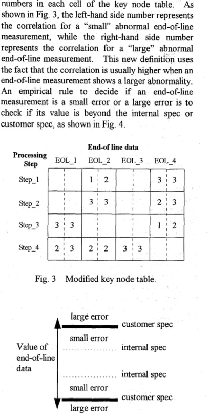
In general, integration engineers use their process physics knowledge and abnormal test data to diagnose the root causes. In order to facilitate the diagnosis process, experienced engineers write down their knowledge into a knowledge table called “key node table.” Fig. 1 depicts one such table used by the industry, which empirically correlates the abnormal end-of-line test data (symptoms) to major process steps (root causes). Numerical values in the table represent the relative rank. When compared columnwisely, number one represents the most probable cause. For example, when EOL-2

shows abnormal values, step-2 is the most probable cause compared to step-4 and step - 1

Processing step Step-1 Step-2 Step-3 Step-4

End-of line data

EOL-1 EOL-2 EOL-3 EOL-4

multiple abnormal end-of-line measurements. 0 Diagnosis process is not robust. The diagnosis

accuracy is highly dependent on the accuracy of the key node table and end-of-line data.

3. Intelligent Diagnosis System

Due to many limitations of the current approach, an intelligent system for the first-cut diagnosis is proposed with the following objectives:

0

0 to automate diagnosis process, 0

o

to enhance the current diagnosis accuracy, to train junior engineers, and

to facilitate knowledge integration / expansion.

Fig. 1 Key node table used by the industry Historically, field engineers use the key node table approach to perform the first-cut diagnosis. Although usefil in some situations, this approach is insufficient. Several problems arise with the use of the key node table:

0 Key node table is empirical. There is great

fbzziness in defining this table by field engineers. o Key node table is incomplete. The accuracy is

highly dependent on engineers’ experience.

0 Diagnosis process is empirical and incomplete.

There is no systematic inference method to determine the root causes when there are

Fig. 2 illustrates the architecture of the proposed intelligent system. It consists of six modules: fuzzy modeling, knowledge base, inference engine, history data base,

U 0

interface, and self-learning. As

shown in Fig. 2, engineers provide abnormal end-of- line test data as the inputs to the system through the I/O interface. The intelligent diagnosis system then calculates each process step’s fault possibility and provides the engineers a list of prioritized causes for firther investigation. Experts’ knowledge or key node table, either old or newly updated, can be also sent to the fizzy modeling module for further processing and stored in the knowledge base.

a@

knowledge

Fig. 2 Architecture of an intelligent diagnosis system.

In general, experts’ diagnosis knowledge contains a lot of qualitative or uncertain information. Traditional probability concept cannot model such information very well. In the fbzzy modeling module, we use fbzzy logic’s possibility concept to model vague information. The resulting information is then stored in the knowledge base.

I I I I I I With the information of abnormal end-of-line data

and knowledge base, each major process step’s fault possibility is calculated in the inference engine. The resulting information can be provided to the users through the I/O interface or sent to the history data base. The diagnosis results together with the real causes can be sent to the self-learning module for hrther knowledge training. This is usefbl when the initial knowledge base is insufficient or incomplete.

I 3 1 3

I I In this paper, three main modules, fbzzy modeling,

knowledge base and inference engine, will be described in detail in the next two sections. The self-learning function is currently performed by experienced engineers by comparing the system’s diagnosis results with the real causes.

Value of end-of-line data

4. Fuzzy Modeling / Knowledge Base

As mentioned earlier, several problems arise with the

use of the key node table. In order to overcome these difficulties, several approaches are used to effectively extract knowledge.

small error

internal spec

internal spec The first approach is to redefine the key node table

by many experienced field engineers. Through group discussion and information exchange, the resulting key node table represents the most complete key node table available. In addition, numerical number in each cell no longer represents the “rank” of the cause in which number one represents the most probable cause. Instead, it is redefined as the “correlation” between the abnormal end-of-line data and corresponding process steps. Here, a higher number represents a strong correlation and a lower number represents a weak correlation. This new definition has two advantages. First, each cell number can be defined individually. Second, the concept of strong, medium and weak correlation can be easily modeled using hzzy logic theory.

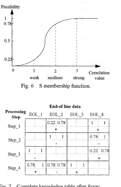
The second approach is to use two correlation

numbers in each cell of the key node table. As

shown in Fig. 3, the left-hand side number represents the correlation for a “small” abnormal end-of-line measurement, while the right-hand side number represents the correlation for a “large” abnormal end-of-line measurement. This new definition uses the fact that the correlation is usually higher when an end-of-line measurement shows a larger abnormality. An empirical rule to decide if an end-of-line measurement is a small error or a large error is to check if its value is beyond the internal spec or customer spec, as shown in Fig. 4.

End-of line data Processing

Step

-

EOL-1 EOL-2

U

Step-1 Step-2 Step-3 Step-4 ~

1996 IEEUCPMT Int‘l Electronics Manufacturing Technology Symposium

349

Fig. 3 Modified key node table.

4-

customer spec

small error large error

customer spec

Fig. 4 A rule to decide small and large errors. The third approach is to include the error direction information into the key node table. Often, the deviation of an end-of-line measurement from its target value may depend on the deviation of a process step’s parameter from its target setting. If the correlation between the two deviations can be derived based on process physics, it can be used in the key node table as shown in Fig. 5 . Here a

positive sign represents a positive correlation and a minus sign represents a negative correlation. This

information also provides the inter-dependence 1

step 4 has a positive error, then EOL-1 and EOL-3 relationship among the end-of-line measurements for a given miss-operated process step. For example, if will have positive errors while EOL - 2 has a negative error.

o.5

Step-1 End-of line data

Processing EOL-1 EOL-2 EOL-3 EOL-4

Step

,

I I I 1

022 0 7 8 1 1

+

4-

+

Step-4

Fig. 5 Correlation between end-of-line and process step's deviations.

-

+

Although the key node table is redefined and more knowledge is extracted based on the first three approaches, the knowledge is still too empirical for fbrther manipulation. The fourth approach is then to transform the correlation numbers into fbzzy logic's possibility using S membership hnction [9]. The S membership function is defined below and is also shown in Fig. 6.

Step-2 I I I I I I 0.22- I I

c

1 1 0 7 8 1 - - 1 2 Correlation 0

weak medium strong value Fig. 6 S membership function.

1 : 1 0.22; 0.78

. . . . ....,.. . . . . ...

-

+

End-of line data

Step-3 Step-4

Fig. 7 Complete knowledge table after fbzzy modeling .

5. Inference Engine

The inference engine computes, by using fuzzy logic operations, the possibility of a process step causing the observed abnormal end-of-line measurements. The inference algorithm is based on comparing the observed abnormal patterns with patterns in the knowledge base (KB). For a given process step, a better match between the two patterns, a higher possibility is assigned to the step.

x 5 a S(X) = 0 2 a + b ='2( ) a < x < - - - - 2 < x < b ( x - b ) 2 __ a + b (1) = 1 - 2 __ 9 = 1 b < x

For a process step i, the possibility of a positive fault is given by:

n

A p v

n

Here, x is the correlation value as defined in the key knowledge table after fizzy modeling is shown in

Fig. 7. j = l

f j = l

node table, and

a

= 0, b = 3 . The complete

<

= @ . A . =

1 1 NI

c

s'y

n = number of abnormal end-of-line measurements N , = number of end-of-line items for step i in the KB

a+.

= cell i j matching factor

Sv = cell ijpossibility in the KB A , = step i weighted sum of possibility

o = step i matching factor

v

1

Notice that the

“+”

sign represents a positive fault, i.e., the step’s parameter is “higher” than the target value. We can also use equation similar to (2) to

calculate the possibility of a step’s negative fault (by using A-). The calculation steps are described in detail below and illustrated in Fig. 8.

Step 1 :

Assume the step i is positively (+) deviated from its target value, then we define:

Calculate the cell matching factor

A’

a+.

= 1 if KB cell i j has the same sign

(+,-) as the sign of the observed end-of-line measurement j

v

a+.

= o

other cases

v

SteD 2: Calculate the weighted sum of possibilitv A

(3)

End-of-line

e-3

1

Determine cell’s matching factor

Calculate step’s fault possibility

-+

7

=

m i A i

Here, S, must be chosen based on whether end-of- Fig. 8 Inference engine calculation steps. line measurementj is a small error or a large error.

SteD 3: Calculate the step matching; factor CO

The purpose of cell matching factor and step matching factor is to evaluate the consistency between the knowledge base (prior information) and the observed end-of-line data.

The cell matching factor evaluates the error direction (4) consistency. The step matching factor evaluates Ni

c

8,

the consistency of the overall error pattern. If the

j = l diagnosis is based only on emphasizing

measurements that deviate but ignoring those that do not, it might bias the decision.

n j = l

a;sY

Cui = Step 4: Step 5 :

Calculate each steo’s fault possibility

P’

Repeat for

P

-

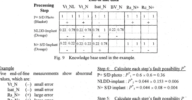
End-of line data Vt NL Vt-N _- Isat-N BV N RS N+ Rc _{- - -} N+ Processing Step P+ S/D Photo planket) NLDD-Implant (Dosage) . . . , . . .

Fig. 9 Knowledge base used in the example.

Example Step 4: Calculate each step's fault possibilitv P'

Five end-of-line measurements show abnormal p+ _ . ~ S/D photo : pfl = 0.6 0.6 = 0.36 values, which are:

Vt-N (-) small error Isat-N (-) small error

R s N + (+) large error

Rc N+ (+) large error

R - S W (+I small error

NLDD-implant :

Pfz

= 0.044 x 0.153 = 0.006 N+ S/D implant : P', = 0.044 x 0.08 = 0.004

Step 5 : Calculate each step's fault possibility P -

P+ S/D photo :

P

- = 0.2 x 0.2 = 0.04

NLDD-implant : P - , = 0.156 x 0.54 = 0.08 N+ S/D implant : P - , = 0.444 x 0.84 = 0.37

So the three most possible steps are:

N+ S/D implant (negative error,

P

- 3 = 0.37)

NLDD-implant (negative error, P - = 0.08)

Part of the knowledge base is shown in Fig. 9. Based on the information, we want to know which process steps are the causing steps.

Step 1 : Vt-N

P+ S/D photo :

NLDD-implant : 6. Data Validation

A+=

1 0 0 0 0 Twenty three test cases are carefblly selected from

N+ S/D implant : historical lot data by experienced field engineers to

A'=

1 0 0 0 0 validate the proposed diagnosis system and to

explore its properties. The metric for validation is Step 2: Calculate the weighted - sum OfpossibilitvA defined as fol~ows. If the top (second, third)

P+ S/D photo : possible cause of a case identified by the diagnosis

= (0 1 + 1 1 + 1 1 + 1 1 + 0 0 ) 5 = 0.6 system matches the real cause, a score of one (0.5,

NLDD-implant : A , = (1 x 0.22) / 5 = 0.044 0.25) is given to the test case. Our validation

focuses on the inference engine and knowledge base. N+ S/D implant : A , = (1 x 0.22) / 5 = 0.044

Improvements in these two modules are carried out along with the validation by individual cases.

Step 3:

P+ SD photo :

w1

= (1+1+1) / (l+l+l+l+l) = 0.6

The validation starts with the baseline diagnosis NLDD-implant :

system, where the inference engine does not include

w z

= (0.22) / (0.22-1-0.22-tO.78-tO.22) = 0.153

consideration of step matching factor ( w i in Eq. 4)

N+

S/D implant :

w3 = (0.22) / (0.22+0.22+0.22+1+1) = 0.08 and the knowledge base of version 1.0 is used. Validation result of the first 14 test cases is depicted Calculate the cell matching factor

'

A

Isat - N Rs - N+ Rc-N+ R s - W P+ S/D photo (positive error, P+l = 0.36)

A+=

0 1 1 1 0

Calculate the step matching factor w

by the solid line in Fig. 10, where the system diagnoses the actual causes as top possible causes in half of the cases and the average score is 0.55. Analysis of the misdiagnosed cases (cases 6, 7, 9, 1 1, 12 and 14) indicate two types of deficiency in the baseline system, one suggesting inclusion of the step matching factor into the inference engine and the other suggesting enrichments of the knowledge base. Details are described as follows.

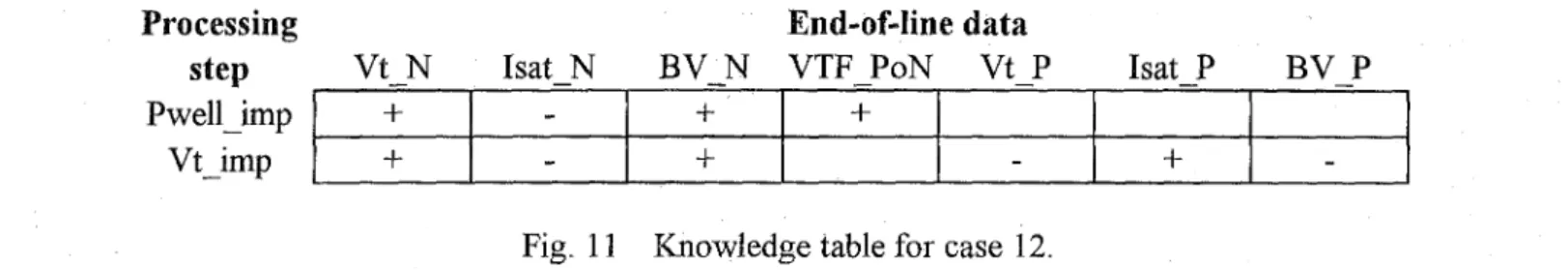
The calculated values are: Vt-imp: A = 1.0

Pwell-imp : A = 0.75

However, if Vt-imp is really the cause, we should observe abnormal values for BV N, Vt-P, Isat P and BV P (Fig. 11). These motivate the addition of the step matching factor into consideration as described in section 5. The newly calculated possibilities are:

Pwell - imp :

Vt-imp :

Diagnosis results of the revised inference engine are depicted by the dash line in Fig. 10, where improvements in cases 9, 1 1 and 12 are obvious and there is no loss of diagnosability in other cases; the

P

=

wA

= 0.56 x 0.75 = 0.42

P =

wA

= 0.36

1 3 5 7 9 1 1 1 3

Case number

Fig. 10 Validation results for knowledge base version 1 .O and inference engine without step matching factor (solid line) and with step matching factor (dash line).

Inference engine

In the original inference engine, the possibility of a process step being the cause of fault is calculated using the weighted sum of possibility ( A . in Eq. 3).

With this method, the step's fault possibility is based only on the end-of-line measurements that deviate from their respective target values. The prior information about the error pattern, i.e., which measurements should deviate in what way when a

process step goes wrong, is not utilized. In other words, the diagnosis is biased by overemphasizing on measurements that deviate but ignoring those that do not. Misdiagnosis in cases 9, 11, and 12 is due to such a deficiency.

I

Specifically, in case 12, the Isat-N value is seriously higher than target (positive and large error) and Vt-N is slightly low. By merely looking at the deviations and using weighted sum of possibility A ,

we deduce that Vt

-

imp is the most possible cause. The true cause Pwell-imp, however, has a lower A

than that of Vt-imp.

average score goes up to 0.64. Knowledge base

Misdiagnosis of cases 6, 7 and 14 does not improve with the revised inference engine because of insufficient or inaccurate knowledge base. For example, the P+-blanket step is the true cause of case 6 but it is not in the knowledge base of version

1

.o.

To overcome the above deficiencies, more detailed process steps are added to the knowledge base, which increases from 34 to 132 in the validating process. Misdiagnosis due to missing steps in the knowledge base is therefore largely eliminated. Diagnosis result obtained by using the revised inference engine and knowledge base version 2.0 over 23 cases are given in Fig. 12, where the first 14 cases are the same cases as those in Fig. 10. Significant improvements in cases 6, 7 and a small improvement in case 14 can be observed while at the price of deterioration in cases 5 , 8, 9, 11 and 12. The average score of the first 14 cases slightly goes up from 0.64 to 0.66 and is about 0.68 overall. To sum up, in 13 cases the real cause is identified as the top cause, in 4 cases as the second and in 3 cases as the third. Out of the 23 studied cases, version 2.0 of the system identifies the real causes as the top three causes in 20 cases.

Pwell imP

1

+

-

+

+

Fig. 11 Knowledge table for case 12.

- 1

Vt-imp

The deterioration is mainly due to the inaccurate parameters in the knowledge base. For example, in case 8 step Polyghoto/etch (small poly gate length) can be identified as the cause of symptom pattern of low Vt-N and large Isat-N by applying two physical rules,

a Vt a L (Lis poly gate length)

a Isat a 1/L

Our diagnosis system only ranks Poly_photo/etch as 2nd possible because the weighting is inaccurate which makes step NLDD the top possible and is

inconsistent with the reality. Parameters of hture knowledge base should be adjusted to better reflect engineers’ knowledge about the basic physical relationship.

I I I I I I

+

-

+

-

+

-

2.0 of the system identifies the real causes as the top three causes in 20 cases. Our analysis indicates that the inference engine is robust but the knowledge base is insufficient, A short-term improvement strategy is to periodically update the knowledge base by field engineers based on lessons learned from the case study. Future long-term improvement plan might use neural network to perform the self- learning.

References

[l] K. Saito, M. Sakaue, T. Okubo, and K. Minegishi, “Application of Statistical Analysis to Determine the Priority for Improving LSI Technology,” IEEE Transactions on Semiconductor Manufacturing, vol. 5, no. 1, February 1992.

[2] S. Saxena and A. Unruh, “Diagnosis of Semiconductor Manufacturing Equipment and Processes,” IEEE Transactions on Semiconductor Manufacturing, vol. 7, [3] K. Funakoshi and K. Mizuno, “A Rule-Based Process Flow Validation System with Macroscopic Process

E

3

0.5

m Simulation,” IEEE Transactions on Semiconductor

Manufacturing, vol. 3, no. 4, February 1990.

[4] S. B. Dolins, A. Srivastava and B. E. Flinchbaugh, 0.25

“Monitoring and Diagnosis of Plasma Etch Processes,”

0 IEEE Transactions on Semiconductor Manufacturing,

[ 5 ] R.J. Kuo, “Intelligent Diagnosis for Turbine Blade Faults Using Artificial Neural Networks and Fuzzy 1

0.75 no. 2, May 1994.

1 4 7 10 13 16 19 22 vol. 1, no. 1, February 1988. Case number

Fig. 12 Validation results for knowledge base version 2.0 and inference engine with step matching factor.

7. Conclusions

In this paper, we describe an intelligent diagnosis

system for a first-cut end-of-line diagnosis function. The system uses information of abnormal end-of-line data and fkzzy logic-based knowledge base to calculate each major step’s fault possibility.

The intelligent diagnosis system has been validated against 23 real fab cases. Results show that version

Logic,” Engineering Applications of Artificial Intelligence, vol. 8, no. 1, 1995.

N. Kartan, I. Flood, and T. Tongthong, “Integrating Knowledge-based Systems and Artificial Neural Networks for Engineering,” Artificial Intelligence for Engineering Design and Manufacturing, vol. 9, 1995.

H C Fu and J.J. Shann, “A Fuzzy Neural Network for

Knowledge Learning,” International Journal of Neural Systems, vol. 5 , no. 1, March 1994.

R.K. Ramamurthi, “Self-Learning Fuzzy Logic System for In Situ, In-Process Diagnostics of Mass Flow

Controller,” IEEE Transactions on Semiconductor Manufacturing, vol. 7, no. 1, FebruaIy 1994.

[9] D. Driankov, H. Hellendoom, M. Reinfrank, An

Introduction to Fuzzy Control, Springer, 1993.

[6]

[7]

[SI

1996 IEEEICPMT Iflt‘l Electronics Manufacturing Technoloav Svmnnnillm