P e r g a m o n Copyright©1997 Elsevier Science Ltd Printed in Great Britain. All rights reserved
P I h S0898-1221(97)00210-1 0898-1221/97 $17.00 + 0.00
A Heuristic Approach to Generating File
Spanning Trees for Reliability Analysis
of Distributed C o m p u t i n g Systems*
D E N G - J Y I C H E N , R U E Y - S H U N CHEN** AND T I E N - H S I A N G H U A N GInstitute of Computer Science and Information Engineering National Chiao Tung University, Hsinchu, Taiwan, R.O.C.
(Received and accepted October 1994)
A b s t r a c t - - T h e reliability of Distributed Computing Systems (DCS) in terms of Distributed Pro- gram Reliability (DPR) and Distributed System Reliability (DSR) has been studied intensively. Cur- rent reliability algorithms available for the analysis of DPR and DSR include MFST, FARE, FST, and FST-SPR. This paper presents a reliability algorithm, called HRFST, that eliminates the need to search a spanning tree during each subgraph generation. The HRFST algorithm reduces both the number of subgraphs (or trees) generated and the actual execution time required for analysis of DPR and DSR. Examination of several sample cases shows that the HRFST algorithm is more efficient than the FST-SPR algorithm.
g e y w o r d s - - D i s t r i b u t e d Computing Systems (DCS), Distributed Program Reliability (DPR), Distributed System Reliability (DSR), Reliability.
1. I N T R O D U C T I O N
In reliability analysis of Distributed Computing Systems (DCS), V.K.P. K u m a r has proposed a very useful notion called a Minimal File Spanning Tree (MFST) and developed an algorithm called M F S T to find MFSTs within a graph [1,2]. T h e M F S T algorithm takes two passes to obtain the reliability of PDS. Pass 1 is to obtain the multiterminal connections for every MFST. Pass 2 is to use an algorithm called SYREL [3] to compute the equivalent reliability expressions by the multiterminal connections of every MFST. To improve the M F S T algorithm, A. K u m a r developed an algorithm called FARE (Fast Algorithm for Reliability Evaluation) [4,5] to compute the D P R and DSR. T h e FARE algorithm uses a connection matrix to represent each M F S T and proposes some simplified techniques for speeding up the analysis process. To further improve the evaluation speed, we also proposed the F S T - S P R algorithm for reducing the number of subgraphs generated during reliability evaluation [6]. In [6], the F S T - S P R algorithm was compared with the M F S T and FARE algorithms to show its performance advantage. T h e basic idea behind the F S T - S P R algorithm is to make subgraphs generated completely disjoint, so t h a t no replicated subgraphs are generated during the reliability evaluation process. In order to generate disjoint subgraphs, we have to search a spanning tree from the current graph and then cut each edge in the spanning tree disjointly to produce the disjoint subgraphs. This process is repeatedly applied to each subgraph generated until a File Spanning Tree (FST) is found or no edge is reached. *This research work was supported in part by the National Science Council of the R.O.C. and in part by the C h u n g San Institute of Technology, ~iwan, R.O.C.
**Author to w h o m all correspondence should be addressed.
Typeset by ~4.A48-TEX 115
116 D.-J. CHEN et al.
Therefore, to find a spanning tree from each generated subgraph can be computationally costly and time consuming.
In this paper, we present a reliability algorithm called HRFST that eliminates the need to search of a spanning tree during the generation of each subgraph. The HRFST algorithm reduces both the number of subgraphs (or trees) generated and the actual execution time required for the analysis of DPR and DSR. Examination of various sample cases clearly shows that the HRFST is more efficient than the FST-SPR algorithm.
2. P R E V I O U S W O R K
The notation and definitions used in [7] are recalled here for consistency.
2 . 1 . N o t a t i o n
x~: a node representing a processing element i x i j : a link between processing elements i and j p ~ j ( q i j ) : probability that t h e link xi,j is working (failure)
t: a subgraph, which can be a tree or forests of the DPS graph (the trees and forests are represented by sets of nodes and links)
Fi: the d a t a file i
Pi: the distributed program i
FAI: the set of d a t a files available at processing element xi FAt: the set of d a t a files available by subgraph t
PAi: the set of programs available at processing element x~ PAt: the set of programs available by subgraph t
PN: the set of programs that need to be executed in the DPS FNi: the set of d a t a files needed for program i to be executed
FN: the set of d a t a files needed for several programs to be executed in t h e DPS
LSt: a set of links t h a t represents the links' state in the subgraph t; the s t a t e of each
link in the set is:
failure if ~ E LSt working if xi,j E LSt do not care otherwise
STt: a set of links t h a t can be used to represent a spanning tree of t h e subgraph t
PRt: a probability expression denoted by p~,j or q i j t h a t represents the probability of the subgraph t containing a working spanning tree
Rt: the reliability of the subgraph t R: the reliability of the DPS
2 . 2 . Definitions
DEFINITION 1. An F S T is an File Spanning Tree that connects the root node (the processing element that runs the program under consideration) to some other nodes such that its vertices hold all the necessary data files for the programs to be executed.
DEFINITION 2. An M F S T is a minimal FST such that there exists no other FST which is a subset of it.
DEFINITION 3. A p r o b a b i l i t y space is composed by all possible states of the links (working, failure, or do not care).
DEFINITION 4. A p r o b a b i l i t y g r a p h is a graph that has a probability space associated with it. For the original graph, the probability is assumed to be 1 (all links do not care). Also, the probability space of a subgraph that will be equal to the sum of the probability space of all subgraphs generated by this subgraph.
DEFINITION 5. A subgraph t is satisfied means that the data files and programs available by subgraph t can execute the distributed program successfully.
(FAt D_ FN,
andPAt D_ PN, and
the failure links will not affect the program's execution.)DEFINITION 6. A subgraph t may generate several subgraphs by cutting its links. Then the subgraph t is called a parent subgraph and the subgraphs generated from subgraph t are called child subgraphs of subgraph t.
2.3. T h e F S T - S P R A l g o r i t h m
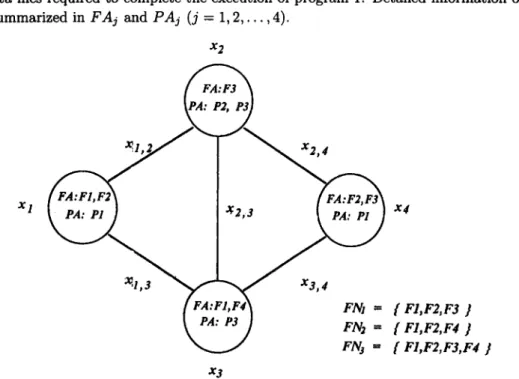
Consider the distributed processing system in Figure 1, there are four processing elements (xt, x2, x3, x4) connected by links xl,2, xl,3, x2,3, x2,4, and x3,4. Processing element Xl contains two data files (F1 and F2) and can run program 1 directly to communicate with other nodes to access data files required to complete the execution of program 1. Detailed information on each node is summarized in
FAj and PAj
(j = 1, 2 , . . . , 4).x2
~1,3 ~
X3,4
FN2 = [ F1,F2,F4 ]
FNj = [ F1,F2,F3,F4 ]
x3
Figure 1. A simple DPS with four processing elements.
An outline of the FST-SPR algorithm used to compute the DPR and DSR presented here. For a more detailed treatment, readers are referred to [6].
Step 1. Perform reliability-preserving reduction on the original DPS graph. Step 2. Find a spanning tree from the reduced DPS graph.
Step 3. Cut each link from the spanning tree (obtained from Step 1) so that the resulting subgraphs are all completely disjoint.
Step 4. Check whether each the resulting subgraph contains an FST. If so, then repeat Steps 1 to 4 until the resulting subgraph contains no FST or the resulting subgraph contains no link.
Step 5. For all the subgraphs generated during the cutting process, sum all the probability subgraphs that contain an FST by adding all the associated probability spaces to obtain the final reliability.
Subgraphs generated using the FST-SPR reliability algorithm are completely disjoint, and hence, no replicated subgraphs (or trees) will be generated. In [6], the FST-SPR algorithm was compared with MFST [1] and FARE [5] to show its performance advantage in the analysis of D P R and DSR.
118 D.-J. CMEN e t al.
3. T H E H R F S T A L G O R I T H M
3.1. O b s e r v a t i o n s o n t h e F S T - S P R A l g o r i t h m
When we study the FST-SPR algorithm carefully, we find that a spanning tree must be found each time for a subgraph is generated (as shown in Step 2 of the FST-SPR algorithm). This implies that the number of times the spanning tree generation procedure is invoked is equal to the number of subgraphs generated. In the worst case, the computation cost will be L!, where L is the number of links in the first spanning tree identified in the original graph. Thus, the cost to find a spanning tree in the FST-SPR algorithm is high.
The purpose of finding a spanning tree is to see if the current subgraph can run the distributed program successfully (whether it contains all the data files required for the execution of the distributed program under consideration). If it can, then a disjoint-cutting process is performed to generate disjoint subgraphs from the current subgraph. If it cannot, then the subgraph generation is stopped. This implies that a spanning tree that can run the distributed program successfully will also be an FST and that it will take more time, in general, to run the distributed program, since the number of nodes and links of a spanning tree is greater than the number of nodes and links of an FST. Thus, using the spanning tree to run the distributed program will take more time and generate more subgraphs than that of the FST during the analysis of DPR and DSR.
Based on the above observations, we suggest that if we can find a way to choose an FST together with an appropriate cutting approach to generating subgraphs, then both the computation time and the number of subgraphs can be reduced. This suggestion can be justified easily. Consider the example in Figure 2, and suppose links i l ,
L2,..., L5
in graph A are a spanning tree. Then five disjoint subgraphs will be generated from graph A by applying the FST-SPR algorithm. Suppose links L1, L2, L3 in the same spanning tree are an FST for a distributed programPj.
Then the operation of links L1, L2, L3 in graph A will be enough for successful execution of programPj.
Thus, finding the FST instead of the spanning tree for the disjoint-cutting process will generate fewer subgraphs. The difference between the use of an FST and a spanning tree for subgraph generation is shown in Figure 2.graph A graph A
L ~ ] b4spanning t r ~ : ~ FST :
[ fl I[ 11 ID
r
I
F i g u r e 2. Difference between the use of s p a n n i n g tree and F S T .
3.2. T h e C o n c e p t u a l F o u n d a t i o n o f t h e H R F S T A l g o r i t h m
Once the motivation is understood, we need to construct a method of finding an FST with reasonable cost and then to apply the disjoint-cutting process to generate subgraphs. The most straightforward approach is to use the MFST algorithm to find an FST. This is not a good solution, however, since we have been trying to avoid generating replicated trees (subgraphs), in order to reduce the computation time. Thus, a new approach must be developed.
Here we will present a new method of finding an FST. The basic idea of the method is to find a heuristic cost function to compute the cost of each link x i j in terms of data files and programs resident in nodes xi and xj. Through the cost function analysis, we will he able to understand,
which connecting between nodes will offer us a good chance of obtaining an FST. T h e heuristic cost function is defined below.
cost(x~j) = # ( F N ( F A , U F A j ) ) + # ( P N - (PA~ (J P A j ) ) ,
where "-" is the difference set and " # " is the number of sets.
Therefore, cost(xij) = 0 means t h a t if link x i j is selected then there is a good chance t h a t an F S T is in subgraph x j , x~d, x j . Rules for selecting links are listed below.
Rule 1. Always choose the link t h a t has the minimum cost in the graph.
Rule 2. If there are two or more links with the minimum cost, then choose the one whose connecting nodes have the least replicated d a t a files and programs among those under consideration.
Rule 1 indicates that we should use the mos't important link as the factor for the probability partition process; Rule 2 tells us t h a t connecting two nodes that have the least-replicated d a t a files and programs will decrease the costs of the adjacent links. This will enable an F S T to be found as soon as possible.
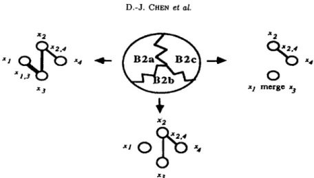
Consider the DPS in Figure 1 for the analysis of DPR1. T h e costs of links Xl,2, Xl,a, x2,3, x2,a, and x3,4 are, based on the cost function defined above, 0, 1, 2, 1, and 0, respectively. According to the link selecting rule, link Xl,2 is selected to be cut for the generation of subgraphs. Since its cost is zero, there is only one subgraph generated by the original graph. T h e probability space after this partition is shown in Figure 3.
x 3 x 3
Figure 3. The probability space of the original graph.
If we continue the analysis process, the costs of links x1,3, x2,z, x2,4, and xa,4 are now 1, 2, 1, and 0, respectively. Since the link Xa,4 has the minimum cost (zero), the subgraphs of portion B are the subgraph B without link xa,4 (shown by portion B2). T h e probability space after this partition is shown in Figure 4.
Xl q ( ~ ~4 ~ ~ , , ~ xl x4
1.30x3,4
1,3
(..)
x 3 x 3
Figure 4. The probability space of the portion B.
T h e portion B2 now has to be split. T h e costs of links xl,a, x2,z, and x2,4 are 1, 2, and 1, respectively, so the first link to be cut is x l , z . Since the cost of link Xl,a is not zero, another link should be selected to be cut for generating the second subgraph. Because of the disjoint property, the second subgraph of subgraph B2 should merge the nodes xl and xz, and now the costs of links xz,3 and x2,4 are 0 and 1. Since the cost of link x2,z is the minimum and is zero, then the
120 D.-J. CHEN et al.
x l Q ( ~ ;4 ~ ~ x4
x_, ~1 merge x 3
x 3
Figure 5. The probability space of the portion B2.
link to be cut in the second subgraph is x2,3. The probabiliW space after this partition ks shown in Figure 5.
T h e P R t of every subgraph can be computed according to the LSt and a set called W O R N t , which is the set of the links to be cut by the subgraphs (multiply Pi,j if x i j E L S t or x i j E W O R K t , multiply qi,j if ~ E LSt). Finally, we sum all the P R t ' s to obtain the reliability of the DPS.
3.2. T h e C o m p l e t e H R F S T R e l i a b i l i t y A l g o r i t h m
T h e H R F S T algorithm is different from the F S T - S P R algorithm; it is described informally below.
1. Perform as many reductions on the current graph as possible and compute the cost of each link while carrying out the reductions.
2. If there is any single node that contains all data files and programs required, then remove current graph from TRY, store the current graph in the list FOUND, and go to Step 5. 3. Remove the current graph from TRY. If it has no links that can be cut, then store the
current graph in the list FOUND and go to Step 7.
4. Use Rule 1 and Rule 2 to select a link xi,j. Cut the selected link xi,j from the current graph to generate the first subgraph. Connect nodes xi and xj and perform reductions if necessary. Repeat the same process to get a link xk,t and cut link xk,t to generate the second subgraph, until a link Xm,n with cost zero is chosen to produce the ~t t h child subgraph.
5. Set the links chosen in Step 4 to in the current graph. This implies that the current graph contains at least one FST. Add the current graph and the working links to FOUND. 6. Check each subgraph generated in Step 4 and add the candidate F S T subgraphs to the
list TRY.
7. For each subgraph in TRY, apply Steps 1 to 6 repeatedly until list TRY is empty. 8. All the FSTs of each size are now stored in the list FOUND.
T h e formal algorithm is presented below. H R F S T ALGORITHM. b e g i n step 1: initialization t = original graph ; T R Y = { t } ; FOUND = f ;
LS,
=f;
F N = F N i tJ F N i (where program i • P N ) ;R = O ;
step 2 : compute_cost(t) ; step 3 : generate subgraphs
r e p e a t
3.1.1 get a graph t from TRY and remove t from TRY ; 3.1.2 reduction step repeat degree-l_reduction(t) ; degree-2_reduction (t); series_reduction(t) ; parallel_reduction(t) ; unsatisfied_connected_components_deletion(t) ; u n t i l no reduction happen 3.2 checking step
i f there is any single node i where FA~ D_ F N and P A i 2 P N t h e n set P R t according to L S t add t to FOUND; continue; find any connected component i in t such that
FA~ 2 F N and PA~ C_ P N ;
i f any connected component i exists t h e n add t to FOUND ;
else continue ; 3.3 cutting step
add subgraph (t, WORKt) to TRY ; for all link x~,j E WORKt ;
P R t = P R t * Pi,j ; o d
u n t i l (TRY = f) step 4 : compute reliability
for all t E FOUND R = R + P R t ; o d
e n d
procedure subgraph (t, WORKt) b e g i n W O R K t = y
repeat
child *-- t ; PRchild = P R t ; LSchild : LS~ ;child 4-- nodes_merged( child, W O R K t ) ; f o r all x~,j e W O R K t d o
PRchild = PRchild * p~,j ; o d
xi,j *-- m i n _ c o s t l i n k ( c h i l d ) ; child ~ cut_link(child, xi,j) ; CUTchild = {xi,j} ;
PRehild = PRehild * qi,j ; LSehud = LSehad >> {x--~,j} W O R K t = W O R K t >> {x~,j } ; u n t i l (cost(x~,i) = O)
122 D . - J . CHEN et a~.
return(child)
e n d
procedure compute_cost(t) begin
for each link x~,j in subgraph t do
cost(xi,j) = # ( F Y - (FAi t.J F A j ) ) + # ( P g - ( P A i t..J P A j ) ) od
e n d
procedure modify_cost(t, xi,j) begin
cost(xi,j) = # ( F N - (FAi t_J F A j ) ) + # ( B Y - ( P A i U P A j ) ) e n d
procedure min_costAink(t) ; b e g i n
select a link xi,j whose cost is minimum from all the links in subgraph t ;
if there are two or more links with the same minimum cost, then select the one whose connecting nodes have the least-replicated data files and programs.
e n d
procedure series_reduction(t) b e g i n
for all node xi in t
/* similar to t h a t in t h e F S T - S P R a l g o r i t h m */ modify_cost (t, xk,j)
o d e n d
procedure parallel_ reduction(t) b e g i n
for all node xi in t
/* similar to t h a t in t h e F S T - S P R a l g o r i t h m */ modify_cost(t, Xk,j ) o d e n d procedure degree-l_reduction(t) b e g i n /* similar to t h a t in t h e F S T - S P R a l g o r i t h m */ modify_cost ( t, xk ,j ) e n d procedure degree-2_reduction(t) b e g i n
for all node xi in t
/* similar to that in the F S T - S P R algorithm */ modify_cost(t, xk,j)
e n d
procedure nodes_merged(t,old) b e g i n
for all link x i , j E old
/* the same as t h a t in the HRFST algorithm */ for all nodes xk which is a neighbor node of xi
modify_cost(t, xk,i) o d o d e n d procedure unsatisfied_connected_components_deletion (t) b e g i n
for all unsatisfied connected components i in graph t delete all nodes x n in connected component i ; delete all links x i , j in connected component i ; o d
e n d
4. R E L I A B I L I T Y A N A L Y S I S OF D P S U S I N G T H E H F R S T
R E L I A B I L I T Y A L G O R I T H M S
4.1. E x a m p l e
We shall now apply the HRFST algorithm to the DPS in Figure 1 to analyze the DPR1. Splitting snapshots of the subgraphs generated are illustrated in Figure 6.
DPR1 = Pl,2 T ql,2 P3,4 + ql,2 Pl,3 p2,3 q3,4 -{- ql,2 ql,3 P2,3 P2,4 q3,4-
If we assume all the links have the same reliability, 0.9, then DPR1 is equal to 0.99891. To evaluate the DSR, F N = (F1, F2, F3, F 4 ) . Applying the same algorithm, we obtain
DSR -- Pl,2 P2,3 -I- Pl,2 Pl,3 q2,3 T Pl,2 ql,3 q2,3 P2,4 P3,4 + ql,2 Pl,3 P2,3
÷ ql,2 q2,3 P2,4 P3,4 -{- ql,2 ql,3 P2,3 q2,4 P3,4 -b ql,2 ql,3 P2,3 P2,4. Again, if we assume all the links have the same reliability, 0.9, then the DSR is equal to 0.9963. The results obtained by the HRFST algorithm are equivalent to those obtained with the FST-SPR algorithm.
4.2. T h e C o r r e c t n e s s a n d T i m e C o m p l e x i t y o f t h e A l g o r i t h m THEOREM 1. The F S T - S P R a l g o r i t h m is correct.
PROOF. See [7].
THEOREM 2. The H R F S T a l g o r i t h m is correct.
PROOF. The cutting method of the HRFST algorithm is also based on the factoring theorem and is equivalent to the form of the equation
R
R ( G ) = p~,j , pk,l . . . p ~ , z p u , v R ( G n ) + PidPk,l . . . Py,zq~,~ ( Gn )
+ P i , j P k , l . . . q ~ , z R ( G ~ - I ) - t - " " "t- q ~ , j R ( G ~ ) .
Further, the topology meaning of the factors is an FST instead of a spanning tree. Thus, the disjoint property still holds in the HRFST algorithm. All the reduction techniques are also
124 I).-.I. (*,III.;N ¢.'t tg/.
X2
cost(xl,2) ---- 0 ~ A : n o d e s _ m e r g e d
XI ~
X4
cost(xl.3) -- I (~ : parallel reduction
cost(x2,3) -- 2 x3 ® : series reduction
L S =. { } + : degree-2 reduction cost(x2,4) = I W O R K = (x~,2} cost(x3.4) = 0 P R = Pl,2
I
COSt(X1,3) = 1f3 ~ 3
cost(x2,3) ---- 2COSt(X2,4)----
1 L S = {xt--T~.2 C U T = {xl,2} cost(x3,4) = 0 W O R K --- {X3.4} P R - q l ~ p 3 , 4I
c o s t ( x 1 , 3 ) = 1 _ ~ _ COSt(X2,3) ~- 2COSt(X2,4)----
1 L s = ~ { ~ . 2 , ~ } C U T = {x3.4} W O R K = {XI.3,X2,3} P R = q l ~2Pl,3P2.3q3,4 X2 ~ % t ' ~ X4 ---X2.3~-X2,4 O %%
cost(x2
4) =l
O
~ X 3 . 4 X 3 ~ c - ~ s t ( x 3 . 4 ' ) ---- 0 x I A X 3 0 X4 L S = { x l a , xl,3,~---~,4 L S --- {x--l,~xl,3,x-'~,3,x3-"~},4 C U T ~- { x l . 3 } C U T - - - {x2.3} X * W O R K ~- { 3,4 } Fail P R = ql,2ql,3P2,3P2,4q3,4 O O L S - -fff'{,2.xl,3,×3.4,x3.4' }
C U T -- { x 3 / } F a i lFigure 6. The splitting snapshots of the D P R I in Figure I.
reliability-preserving, like those incorporated in the F S T - S P R algorithm. Therefore, the H R F S T
algorithm is also correct. II
T h e K-terminal reliability problem has been s h o w n to be as hard as an N P problem [8]. Unlike the time complexity analysis in the K-terminal reliability problem [0,10], which is statically dependent on the given k-terminal connection, the time complexity of the distributed p r o g r a m
T~ble 1. The file distribution of the DPS. Table 2. The program distribution of the DPS.
Node Files Node Programs
x l F1 x l P1 x2 F2 x2 P4 x3 F3 x3 P2,P3 x4 F4 x4 P2,P3 x s F5 x5 P4 x6 F6 x6 P1
Table 3. The data files required for execution of each program. Program Files Required
P1 F1,F3,F4,F5 P2 F2,F4,F5,F6 P3 F1,F3,F4,F5,F6 P4 F1,F2,F3,F4,F5,F6 x 2 x4 x 2 x4 :~3 x 5 ):3 x 5 (a) (b) x 2 x 4 x 2 x 4 x 3 x 5 x 3 x 5 ( e ) ( d ) x 2 x4 x 2 x 4 x 3 x 5 x 3 x 5 (e) (f)
Figure 7. T h e six kinds of topologies for the six nodes.
reliability problem is dynamically bound to the data flies required for each distributed program. The time complexity of the M F S T and F A R E algorithms presented in [1,2,4,5] is 0(2") in the
worst case, where m denotes the number of links in the graph. However, in practical situation, such cases seldom occur, since once an MFST is found the tree expansion is stopped. The proposed HRFST algorithm uses the graph heuristic cutting technique and incorporates reduction techniques to speed up subgraph generation. The time complexity is quite difficult to quantify since the number of links and nodes may be reduced or merged during the evaluation process. However, by common reasoning, the complexity should be less than that of the MFST and
126 D.-J. CHEN et al.
Table 4. The number of subgraph vs. different topology. P 1 execute at xl. Topology a b c d e f Algorithm FST-SPR 7 13 21 30 104 314 HRFST 6 11 17 23 66 179 P2 execute at x4. Topology a b c d e f Algorithm FST-SPR 7 11 11 30 104 311 HRFST 6 9 9 19 65 175 P3 execute at x3. Topology a b c d e f Algorithm FST-SPR 9 29 49 74 139 402 HRFST 8 26 39 53 92 223 P 4 execute at x2. Topology a b c d e f Algorithm FST-SPR 11 37 56 88 180 471 HRFST 10 31 40 58 105 266
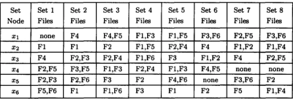
Table 5. Eight sets of data file distributions.
Set Set 1 Set 2 Set 3 Set 4 Set 5 Set 6 Set 7 Set 8
Node Files Files Files Files Files Files Files Files
Xl none F4 F4,F5 F1,F3 F1,F5 F3,F6 F2,F5 F3,F6 x2 F1 F1 F2 F1,F5 F2,F4 F4 F1,F2 F1,F4 x3 F4 F2,F3 F2,F4 F1,F6 F3 F1,F2 F4 F2,F5 x4 F2,F5 F3,F5 F1,F3 F2,F4 F1,F3 F4,F5 none none x5 F2,F3 F2,F6 F3 F2 F4,F6 none F3,F6 F2 x6 F5,F6 F1 F1,F6 F3 F1 F2 F5 F1,F4
F A R E a l g o r i t h m s . O n e good way to c o m p a r e t h e proposed H R F S T a l g o r i t h m w i t h t h e F S T - S P R a l g o r i t h m is b a s e d o n t h e i n t e r m e d i a t e trees (or s u b g r a p h s ) g e n e r a t e d d u r i n g t h e e n t i r e r e l i a b i l i t y e v a l u a t i o n process. I n t h i s way, we c a n tell how m u c h m e m o r y space a n d t i m e is required for t h e different a l g o r i t h m s t o r u n t h e d i s t r i b u t e d programs.
4 . 3 . T h e E f f e c t s o f R e l i a b i l i t y F a c t o r s o n t h e P e r f o r m a n c e o f D i f f e r e n t A l g o r i t h m s T h e file d i s t r i b u t i o n , p r o g r a m d i s t r i b u t i o n a n d topology of a g r a p h all play a n i m p o r t a n t role i n t h e process of a n a l y z i n g t h e reliability of t h e DPS. T h o s e are t h e factors t h a t d e t e r m i n e t h e p e r f o r m a n c e of r e l i a b i l i t y algorithms. I n t h i s section, these factors are used t o c o m p a r e two a l g o r i t h m s : F S T - S P R a n d H R F S T .
4 . 3 . 1 . T h e e f f e c t s o f d i f f e r e n t t o p o l o g i e s
S u p p o s e a D P S c o n t a i n s six processing e l e m e n t s a n d t h e file d i s t r i b u t i o n , p r o g r a m d i s t r i b u - t i o n , a n d t h e necessary files for each p r o g r a m to be executed are as listed i n T a b l e s 1-3. I n F i g u r e 7, t h e r e are six different k i n d s of topologies t o r u n t h e DPPA (i = 1, 2, 3, 4) a c c o r d i n g t o t h e d i s t r i b u t i o n s in T a b l e s 1-3.
Each program is run from some specified sites to communicate with its required d a t a files. T h e number of subgraphs generated in each of the six topologies for each program on different sites is shown in Table 4. T h e comparisons in Table 4, show clearly t h a t the H R F S T algorithm is better in different topologies.
4.3.2. T h e e f f e c t s o f d i f f e r e n t file d i s t r i b u t i o n s
To evaluate the influence of the file distribution on the performance of different algorithms, eight sets of file distributions were selected at random. T h e y are listed in Table 5. A six-node topology is shown in Figure 8 for the eight sets of file distributions to reside in. T h e program distribution and files required for each program to be executed are presented in Tables 2 and 3 above, respectively. T h e comparison results are depicted in Figure 9.
~¢2 "x4
x3 x 5
Figure 8. The topology for file distributions in Table 5.
P2 execute at x3 P I e x e c u t e at x 6 [ --- FST-SPR ,~-RFST ]
I
-~" FST-SPR "~-RFST 35 ./-..
30T • 25.L / ~ . ..._._. 25 " Numberof 2 0 ~ / \ / --gtk ~ Numberof 2 1 ~ subgraphs 1 ! O ~ ; ; I I I I I OI .I I I I I ! I 1 2 3 4 5 6 7 8 1 2 3 4 5 6 7 8Set of file distribution Set of file distribution
(a) (b) P3 execute at x4 P4 ex.ect~ at x5 I .-.FST-SPR 6RFST I
[ "" FST-SPR ~'RFST I
40 ~ 3 5 • . \t 7 .I
\
I - - "
Numberof 25 Numberof ~ " I 2 3 4 5 6 7 8 1 2 3 4 5 6 7 8Set of file distribution Set of file distribution
(c) (d)
Figure 9. Number of subgraphs vs. different file distributions.
4.3.3. T h e e f f e c t s o f d i f f e r e n t p r o g r a m d i s t r i b u t i o n s
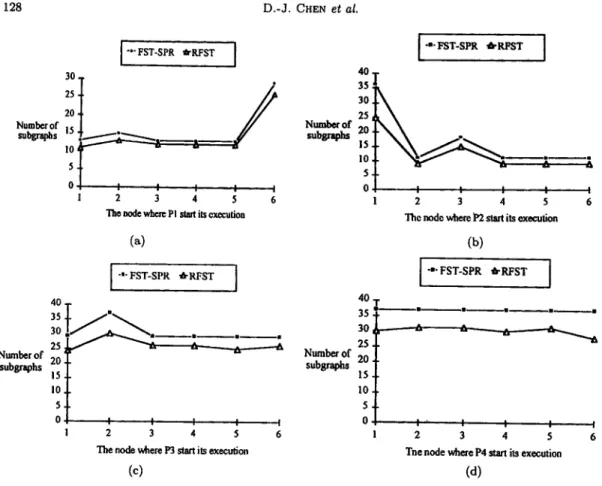
T h e effects of programs running on different nodes of the DPS in Figure 8 are shown in Figure 10. T h e file distribution and data files required for each program to be executed are presented in Tables 1 and 3 above, respectively.
128 D.-J. CHEN et el. ] "'" FST-SPR ~'RFST [ [ "e" FST'SPR '6"RI~T I 30 40 ]- 25 30, 20 25 Number of Number of subgraphs • subgraphs 20,
~l
~ . . 1 5 , to, : i. 5. 0 I I I I 0 I I I I I 1 2 3 4 5 6 2 3 4 5 6The node where Pl start its ~tecutioa The node where P2 start its execution
(a) (b) [ -.- FST.SPR .RFST I I "" FST-SPR ~'RFST ] 40 40 35 . . . . 30 30 ~ ~ -. 25 ~ Numbe# of Nmnberof 20 $ubsraphs 2 0 subgraphs 15 15 I0 I0, 5. I I I I I 0 I' I I I I I 2 3 4 5 6 2 3 4 5 6
The node where P3 start its execution "me node where P4 start its execution
(c) (d)
Figure 10. T h e number of subgraphs vs. different program distributions.
4.4. C o m p a r i s o n of Algorithms
4.4.1. T h e performance of different algorithms on c o m p l e x D P S
The comparison of the performance of different algorithms on complex D P S can be viewed as an objective result, and the more complex the D P S is, the more significant the comparison result is. A n eight node D P S for computing the DPR1, DPR2, DPR3, and DPR4, where the probability of each link is 0.9, is shown in Figure 11. The number of subgraphs generated by different algorithms is depicted in Table 6.
x2 x5
m ~ = {m.ps, F~,/,W
X 4 X7 FN'j = [FI,F2,F4,Fd, FS}
FN 4 = {F2,F3.F4,FS, t~7,FS] Figure 11. A complex DPS with eight processing elements.
A more complex DPS t h a t is a well-known computer n e t w o r k - - A R P A N E T - - i s shown in Figure 12. T h e r e are 21 nodes and 26 links in A R P A NET. Suppose the number of d a t a files
Table 6. The number of subgraphs vs. different programs to be executed. Program P1 P2 P3 P4 Algorithm F S T - S P R 445 334 309 389 HRFST 113 124 118 140 D P R 0.9961182 0.9963265 0.9984532 0.9923256 is 16 a n d t h e n u m b e r o f p r o g r a m s is four. T h e n t h e file d i s t r i b u t i o n , p r o g r a m d i s t r i b u t i o n , a n d files r e q u i r e d for e a c h p r o g r a m t o b e e x e c u t e d a r e as l i s t e d in T a b l e s 7, 8, a n d 9, r e s p e c t i v e l y . A l l t h e s u b g r a p h s g e n e r a t e d for c o m p u t i n g t h e r e l i a b i l i t y o f e a c h p r o g r a m a r e d e p i c t e d in T a b l e 10. S P J LYT~JE-I N C .~A~. A W S C A S E ' A f f O R D
\ I
\ i . _ _ o = /
-
A c U C L A ~ ~ B B N H A R V A R D B L ~ O U C H SFigure 12. ARPA NET.
Table 7. The file distribution of AHPA NET.
Node Files Node Files Node Files
Xl F2 x8 F12 x15 F4 x2 F 3 , F l l z 9 F4 XlS none x3 F7 xl0 F8 x17 F14 x4 F10 x l l F7 xi8 F15 zs F6 x12 F16 x19 F1,F9 xs F13 x13 F10 x20 F5 x7 F12 xla F l l x21 F1,F2
Table 8. The program distribution of ARPA NET.
Node Programs Node Programs Node Programs
Xl P3 xs none Xl5 none
x2 P1 x9 none x16 none
X3 n o n e XlO n o n e X17 n o n e
x4 none Xll none xls P2
x5 none x12 P4 x19 none
xo none x13 none x20 none
x7 none x14 none x21 none
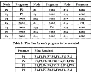
Table 9. The files for each program to be executed.
Program Files Required
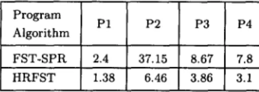
P1 F1,F3,F5,FT,Fg,Fll,F13,F15 P2 F2,F4,F6,F8,F10,F12,F14,F16 P3 F2,F3,F4,F5,F12,F13,F14,F15 P4 FI,F6,F7,F8,F9,F10,F11,F16 T o c o m p a r e t h e a c t u a l e x e c u t i o n t i m e , w e p r e s e n t a D P R i (i = 1, 2, 3, 4) a n a l y s i s u s i n g a n I B M R I S C S y s t e m / 6 0 0 0 t o c o l l e c t e x e c u t i o n t i m e . A l l five a l g o r i t h m s a r e s t r u c t u r e d t o h a v e t h e s a m e I / O a c t i v i t i e s t o e n s u r e t h e f a i r n e s s o f t h e c o m p a r i s o n . T h e s e five p r o g r a m s a r e l i s t e d in t h e
130 D.-J. CHEN et al.
Table 10. The number of subgraphs generated for each program reliability of ARPA NET. Program P1 P2 P3 P4 Algorithm FST-SPR 807 11598 2922 2846 HRFST 356 1274 891 691
appendix. It is clear that the HRFST algorithm outperforms the MFST algorithm. This result justifies our hypothesis that the tedious and time-consuming procedures of checking replicated trees and removing them from the TRY-LIST dominate the overall computation time. The computation times (in seconds) of the DPRi are listed in Table 11.
Table 11. The computation time (computing in seconds) of each DPR, i (i --- 1, 2, 3, 4).
Program P1 P2 P3 P4 Algorithm F S T - S P R 2.4 37.15 8.67 7.8 HRFST 1.38 6.46 3.86 3.1 4.4.2. R e l i a b i l i t y a n a l y s i s o f t w o or m o r e p r o g r a m s e x e c u t e d s i m u l t a n e o u s l y .
To evaluate the results of reliability problem statement 2, based on the DPS in Figure 11, suppose the reliability of each link is 0.9 and several combinations of two or more programs running at the same time are chosen. The number of subgraphs generated by different algorithms is shown in Table 12.
Table 12. The number of subgraphs generated when executing two or more programs together.
Program
P I & P 2 P I & P3 P1 & P 4 P 2 & P 3 P 2 & P 4 Algorithm
F S T - S P R 503 446 563 329 389
HRFST 137 172 192 118 132
D P R 0.9961181 0.9960074 0.9961172 0.9962148 0.9963256
Program
P 3 & P 4 P I & P 2 & P 3 P I & P 2 & P4 P 2 & P 3 & P 4 P I & P 2 & P 3 & P 4 Algorithm F S T - S P R 329 446 563 329 446 HRFST 118 160 156 133 171 D P R 0.9962148 0.9960074 0.9961172 0.9962148 0.9960074
x2, 4 ~ x 4 ,
\ ~,7~2 "~- ] ~ - :¢~.F~.r3j F N s " { ' ~ , I . F $ . F 4 . F . . ~ } I ~ N - - ~'FI,F3oF4,F6J Figure 13. An example of a distributed program running from more than one site.4.4.3. R e l i a b i l i t y a n a l y s i s o f a d i s t r i b u t e d p r o g r a m r u n n i n g from m o r e t h a n o n e site To evaluate the results of reliability problem statement 3, the Figure 13 shows an example in which there are four distributed programs and six data files in the DPS, and all four distributed programs can be executed from two different sites: P1 resides at nodes xl and x6, P2 and P3 reside at nodes x3 and x4, and P4 resides at nodes x2 and Xs. The results of different algorithms are compared in Table 13.
Table 13. The number of subgraphs generated for the example in Figure 13.
Program P1 P2 P3 P4 Algorithm F S T - S P R 35 11 42 46 H R F S T 21 7 23 24 D P R 0.9861766 0.9854047 0.9863232 0.9853018 5. C O N C L U S I O N
In this paper, we have presented a new reliability algorithm, called HRFST, which uses an heuristic cost evaluation function to generate an FST for analyzing the reliability of a distributed computing system. The reliability algorithm eliminates the need to search a spanning tree during the generation of each subgraph. The HRFST algorithm reduces both the number of subgraphs (or trees) generated and the actual execution time required for the reliability analysis of DPR and DSR. Our study of various sample cases and comparisons with the FST-SPR show that HRFST is more efficient than the FST-SPR algorithm.
R E F E R E N C E S
1. V.K.P. Kumar, S. Hariri and C.S. Raghavendra, Distributed program reliability analysis, I E E E Trans.
Software Eng., 42-50 (1986).
2. C.S. Raghavendar, V.K.P. Kumar and S. Hariri, Reliability analysis in distributed systems, I E E E Trans.
on Computer 37 (3), 352-358 (1988).
3. S. Hariri and C.S. Raghavendra, S Y R E L : A Symbolic Reliability Algorithm Based on Path and Cutset
Methods, USC Tech. Rep., (1984).
4. A. Kumar, S. Rai and D.P. Agarwal, Reliability evaluation algorithms for distributed systems, Proc. I E E E
I N F O C O M 88, 851-860 (1988).
5. A. Kumar, S. Rai and D.P. Agarwal, On computer communication network reliability under program execution constraints, I E E E Journal of Selected Areas in Communications, 1393-1400 (1988).
6. D.J. Chen and T.H. Huang, Reliability analysis of distributed systems based on a fast reliability algorithm,
I E E E Trans. on Parallel and Distributed Systems 3 (2), 139-154 (1992).
7. M.S. Lin and D.J. Chen, General graph reduction methods for the reliability analysis of distributed systems,
The Computer Journal 36 (7), 631-644 (1993).
8. M.O. Ball, Computational complexity of network reliability analysis: an overview, I E E E Trans. on Reliability R.35 (3), 230-239 (1986).
9. A. Satyanarayana and K.R. Wood, A linear-time algorithm for computing K-terminal reliability in se- ries-parallel networks, S I A M Journal of Computing 14 (4), 818-832 (1985).
10. K.R. Wood, Factoring algorithms for computing K-terminal network reliability, I E E E Trans. on Reliability P ~ 5 , 269-278 (1986).