以位置為基礎之無線隨意網路路由演算法之研究

國 立 交 通 大 學

應用數學系

碩 士 論 文

以位置為基礎之無線隨意網路路由演算法之研究

On the study of position-based routing

algorithms for wireless ad hoc networks

研 究 生：袁智龍

以位置為基礎之無線隨意網路路由演算法之研究

On the study of position-based routing

algorithms for wireless ad hoc networks

研 究 生：袁智龍 Student：Chih-Lung Yuan

指導教授：陳秋媛 Advisor：Chiu-Yuan Chen

國 立 交 通 大 學

應 用 數 學 系

碩 士 論 文

A Thesis

Submitted to Department of Applied Mathematics

College of Science

National Chiao Tung University

in Partial Fulfillment of the Requirements

for the Degree of

Master

In

Applied Mathematics

July 2012

以位置為基礎之無線隨意網路路由演算法之研究

研究生：袁智龍

指導老師：陳秋媛 教授

國 立 交 通 大 學

應 用 數 學 系

摘 要

On the study of position-based routing

algorithms for wireless ad hoc networks

Student: Carl Chih-Lung Yuan

Advisor: Chiuyuan Chen

Department of Applied Mathematics National Chiao Tung University

Abstract

This thesis considers the problem of designing efficient position-based routing algorithms for wireless ad hoc networks. A routing algorithm is position-based if a node forwards its packet according to the position information (i.e., coordinates in the plane). GREEDY, COMPASS, ELLIPSOID, and FACE are four famous position-based routing algorithms. The former three algorithms run very fast but cannot guarantee message delivery. On the other hand, FACE does not run fast but it guarantees message delivery. It is indeed a challenge to develop an algorithm that can run very fast and can have high delivery rate at the same time. The purpose of this thesis is to propose two such algorithms. Experimental results show that our algorithms are quite good.

Keywords: wireless ad hoc network, position-based routing, delivery guarantee, path dilation, unit disk graph

誌 謝

首先誠摯的感謝指導教授陳秋媛老師，老師細心

的教導使我能夠能夠一窺資工領域的深奧，身上系著

系上繁忙的大大小小事，還是不時的討論指導我正確

的方向，使我在這兩年中獲益匪淺，也學會了很多獨

立研究的方法與知識。

兩年裡的日子，研究室工同的生活點滴，學業上

的討論，一起熬夜趕作業的革命情感等等。感謝眾位

學長姐、同學們以及學弟妹們的互相砥礪，你們的陪

伴讓兩年的研究生活變得更有意義。

最後，我要感謝我的家庭尤其摯愛的雙親，讓我

能夠更致力於學術上的鑽研。

Contents

Abstract (in Chinese) i Abstract (in English) ii

Contents iii

List of Figures iv List of Tables v 1 Introduction 1 2 Preliminaries 5

2.1 The algorithm FACE . . . 6 2.2 The algorithms GREEDY, COMPASS, and ELLIPSOID . . . 7

3 Our main results 7

3.1 Our routing algorithm: HYPERBOLIC . . . 9 3.2 Our routing algorithm: StaticElectricity . . . 13

4 Experimental results 16 5 Concluding remarks 22 References 23

List of Figures

1 (a) Each of GREEDY, COMPASS, and ELLIPSOID can suc-cessfully send a packet from v0 to v5. (b) v1 is a void when v0

sends a packet to v5. . . 3

2 A bad input for FACE; this example is from [2]. . . 4 3 COMPASS fails to reach t from ui for i = 0, 1, 2, 3; this figure

is from [7]. . . 8 4 The tracks of the potential function of GREEDY are

concen-tric circles. . . 10 5 The tracks of the potential function of HYPERBOLIC are

hyperbolas. . . 11 6 The electrostatic field around the destination node. . . 14 7 the electrostatic field with one positive charge and one

nega-tive charge . . . 15 8 The electrostatic field with one positive charge and two

nega-tive charges. . . 15 9 The delivery rate of GREEDY. . . 19 10 The delivery rate of GREEDY, COMPASS, and ELLIPSOID

for UDGs with n = 50 nodes. . . . 20 11 The delivery rate for GREEDY, COMPASS, and ELLIPSOID

for UDGs with n = 70 nodes. . . . 20 12 The delivery rate for GREEDY, COMPASS, and ELLIPSOID

List of Tables

1 The delivery rate of GREEDY for UDGs with n nodes and average degree d. . . . 18 2 The delivery rate (DR) and the average path dilation (P D)

of GREEDY, COMPASS and ELLIPSOID for UDGs with n nodes and average degree d. . . . 18 3 The delivery rate (DR) and the average path dilation (P D)

of GREEDY, COMPASS, ELLIPSOID, HYPERBOLIC, and StaticElectricity for UDGs with n = 50 nodes. . . . 21 4 The delivery rate (DR) and the average path dilation (P D)

of GREEDY, COMPASS, ELLIPSOID, HYPERBOLIC, and StaticElectricity for UDGs with n = 70 nodes. . . . 21 5 The delivery rate (DR) and the average path dilation (P D)

of GREEDY, COMPASS, ELLIPSOID, HYPERBOLIC, and StaticElectricity for UDGs with n = 100 nodes. . . . 21 6 The delivery rate (DR), average path dilation (P D), and

stretch factor (SF ) of GREEDY, HYPERBOLIC, StaticElec-tricity, and FACE-2. . . 22

1

Introduction

We consider routing problems in wireless ad hoc networks which are modeled as unit disk graphs in which nodes are points in the plane and two nodes can communi-cate if their distance is at most some fixed unit. A mobile ad hoc network (MANET) is a system of wireless autonomous hosts that can communicate with each other in the absence of fixed infrastructure. Each node in a MANET can communicate with all other nodes within its transmission range. When two nodes cannot communicate directly, a multi-hop routing path will be used and the message (packet) will route to its destination through intermediate nodes. Throughout this thesis, the terms − message and packet− are used interchangeably. Depending on the forwarding strate-gies in choosing intermediate nodes, routing algorithms for MANETs can be divided into two main categories: topology-based and position-based; see [11]. Topology-based routing algorithms use information about links that exist in the network to perform packet forwarding. Topology-based routing algorithms need to have full information of the topology of the entire network; they usually use routing tables, which have to be pre-computed. Therefore, topology-based routing algorithms have high overhead and scalability problems.

The first position-based routing algorithm was proposed in 1984 in [13]; it is called MFR in [13] and called GREEDY later on. Position-based routing algorithms use the geographical position (i.e., coordinates in the plane) of nodes to make routing deci-sions. In these algorithms, a node forwards packets based on the position information of itself, its neighbors, and the destination of the packet. Therefore a node has to be able to obtain its own geographical position and the geographical position of the destination. Generally, these information are obtained via GPS (Global Positioning

System) and location services. Position-based routing algorithms are also called

ge-ographic routing algorithms (see [6]) and they exhibit better scalability, performance

and robustness against frequent topological changes. Since ad-hoc networks change topology frequently, it is no doubt that position-based routing algorithms outperform topology-based routing algorithms.

The following network characteristics have been used for comparing position-based routing algorithms (see [10]): loop free, distributed operation, path strategy, packet forwarding, path selection metric, memory, guaranteed message delivery, scalability, overhead, adaptive to mobility and additional data. Among these characteristics,

packet forwarding, guaranteed message delivery, and overhead are the most important

ones and are the major concerns of this thesis. For a recent and comprehensive survey of position-based routing algorithms, refer to [10].

There are three main forwarding strategies (see [9, 10]): greedy, restricted

direc-tional flooding, and hierarchical. In greedy forwarding strategy, a route node must

se-lect a locally optimal neighbor with a position progress (advance) towards the packet destination; the metric can be: hop count, geographic distance, progress to desti-nation, direction, power, cost, delay, and a combination of the above. Most greedy forwarding strategies use hop count as their metric. GREEDY [13], COMPASS [7], and ELLIPSOID [5, 16] are three famous greedy forwarding strategies and they all use hop count as their metric (see the next section for these strategies).

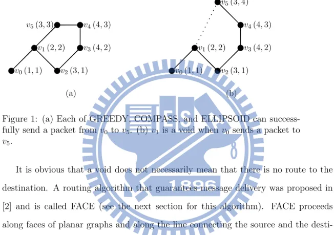
The advantage of greedy forwarding strategy is that it is usually very fast. The drawback of this strategy is that it does not guarantee message delivery. If the message reaches a node which has no closer neighbors to the destination, then a void is reached. When a void is reached, the message has to be discarded if only the greedy forwarding algorithm is used. For example, for the network shown in Figure 1(a),

each of GREEDY, COMPASS, and ELLIPSOID can successfully send a packet from

v0 to v5 and the routing path is v0, v1, v5. However, if the network turns out to be

the one in Figure 1(b), then none of GREEDY, COMPASS, and ELLIPSOID can successfully send a packet from v0 to v5 and v1 is a void.

w_{v0(1, 1)} w_{v1(2, 2)} w_{v2(3, 1)} w_{v3(4, 2)} w_{v4(4, 3)} w v5(3, 3) (a) .. .. .. .. .. .. w_{v0(1, 1)} w_{v1(2, 2)} w_{v2(3, 1)} w_{v3(4, 2)} w_{v4(4, 3)} w_{v5(3, 4)} (b)

Figure 1: (a) Each of GREEDY, COMPASS, and ELLIPSOID can success-fully send a packet from v0 to v5. (b) v1 is a void when v0 sends a packet to

v5.

It is obvious that a void does not necessarily mean that there is no route to the destination. A routing algorithm that guarantees message delivery was proposed in [2] and is called FACE (see the next section for this algorithm). FACE proceeds along faces of planar graphs and along the line connecting the source and the desti-nation. Therefore the underlying network must be a planar graph; to apply FACE, a planarization algorithm must be performed in advance. FACE uses the right hand rule and has to explore the complete boundary of faces. FACE usually has large path dilation; therefore it takes a longer time and is unsatisfactory. To overcome this problem, its well-known improved version, called GREEDY-FACE-GREEDY (GFG) is described in [2]. GFG applies greedy forwarding as much as possible; when a void is reached, a recovery procedure is done through face forwarding; after a void

is bypassed, the strategy is switched back to greedy forwarding again (see also [3]). Such a recovery procedure makes the forwarding strategy a hybrid. See [10] for other hybrids.

The drawback of GREEDY-FACE-GREEDY is that a planarization algorithm has to be performed in advance in order to run FACE and when the input is bad, FACE may have large path dilation (see Figure 2). To overcome this drawback, in this thesis, we will propose two position-based routing algorithms. Both of our al-gorithms are hybrids: the first one is called GREEDY-HYPERBOLIC-GREEDY (or HYPERBOLIC for short) and the second one, GREEDY-StaticElectricity (or Static-Electricity for short). Both HYPERBOLIC and StaticStatic-Electricity use hop count as the metric and apply greedy forwarding as much as possible; when a void is reached, a re-covery procedure is done through HYPERBOLIC or StaticElectricity (see Section 3); after a void is bypassed, the strategy is switched to greedy forwarding again. Notice that both HYPERBOLIC and StaticElectricity do not involve face forwarding and therefore no planarization algorithm is needed. Both HYPERBOLIC and StaticElec-tricity will be compared with GREEDY, COMPASS, and ELLIPSOID. To evaluate the relative performance of these algorithms, we will consider their packet delivery rates and path dilations. Experimental results show that both HYPERBOLIC and StaticElectricity have excellent performance.

Figure 2: A bad input for FACE; this example is from [2].

brief description of FACE, GREEDY, COMPASS, and ELLIPSOID. Section 3 con-tains our algorithms. Section 4 consists of experimental results. Concluding remarks are given in the last section.

2

Preliminaries

This thesis actually considers local routing algorithms, which are position-based routing algorithms satisfying the following three conditions:

• At each point in time, we know position of the starting position and

the position of the destination. In addition, only a constant number of identifiers can be kept in nodes of our network. No point in time do we have full information of the topology of the entire network.

• At each node v, we can use local information stored in v regarding its

neighbors, and the edges connecting v to them. By using this local information plus the information stored in our local memory, an edge incident to v is chosen and traversed until its second endpoint has been reached, unless that is v is the destination, in this case we stop.

• We are not allowed to change the local information stored at a node v.

Notice that once we have left a vertex and if we return to this vertex, we will not be able to determine that we have visited this vertex, unless its identifier is one of the ones carried in our local memory.

A wireless ad hoc network is often modeled as a unit disk graph. Our graph terminologies are standard and we will follow [15]. We suppose the given wireless ad

hoc network contains n nodes and the transmission range of each node is the same (say, r). Two nodes are connected by an edge if the Euclidean distance between them is at most r. The resultant graph is called a unit disk graph. For convenience, the set of neighbors of a node v is denoted by N (v). Let N [v] = N (v)∪ {v}, which is also called the closed neighborhood of v. The line segment between two nodes u and v is denoted by uv and the distance between u and v is denoted by d(u, v). Throughout this section, let s denote the source node, c denote the current node, x denote a neighbor of c, and t denote the destination node.

2.1

The algorithm FACE

FACE (face routing, face forwarding) is also called perimeter routing. The original face routing was called Compass Routing II and was proposed in [7]. There are many improvements of it; Face-2 and AFR (Adaptive Face Routing) are two examples [2]. As was mentioned before, one drawback of face routing is: it usually has large path dilation (the routing path usually is much longer than the shortest path). To reduce the path dilation, hybrid routing algorithms have been proposed. These hybrids combine greedy routing with face routing; GFG (GREEDY-FACE-GREEDY), GPSR (Greedy Perimeter Stateless Routing), and GOAFR are some examples.

Recall that face routing is designed to overcome the inability of greedy routing to guarantee message delivery. To achieve this goal, position information are used to extract a planar subgraph so that routing can be performed on the faces of this subgraph and along st. In face routing, packets are relayed through a sequence of adjacent faces, which are intersected by st. Face routing uses the right hand rule to explore the faces (this is analogous to exploring a maze by keeping one’s right hand on the wall). In the original face routing, the entire perimeter of a face is traversed

and at the intersection point p of st with the perimeter which is closest to t, routing switches to explore the face that shares p. Another version of face routing is to switch to explore the face that shares p where p is the first intersection point of st with the perimeter; this version is also called Face-2 [2].

2.2

The algorithms GREEDY, COMPASS, and ELLIPSOID

In GREEDY, a node forwards the packet to its neighbor which is closest to the destination (i.e., the packet is forwarded to the neighbor with the greatest progress). In COMPASS (compass routing, also called directional routing), a node forwards the packet to a neighboring node such that the angle formed between the current node, next node, and destination is minimized. ELLIPSOID is similar to GREEDY except that among the nodes in N (c), ELLIPSOID will choose the node x which minimizes d(c, x) + d(x, t) and GREEDY will choose the node x which minimizes

d(x, t). ELLIPSOID usually finds a path that is close to the line segment st.

GREEDY, COMPASS, and ELLIPSOID are simple and quick and usually find the shortest routing path. However, none of them guarantees message delivery. In particular, in [7], it has been shown that even in cases when the networks are triangu-lations, COMPASS does not guarantee message delivery; see Figure 3. ELLIPSOID is known to fail very easily when the network has two nodes that are very close to each other.

3

Our main results

The purpose of this section is to propose our main results: two local routing algorithms, which are called HYPERBOLIC and StaticElectricity. Again, throughout

Figure 3: COMPASS fails to reach t from ui for i = 0, 1, 2, 3; this figure is from [7].

this section, let s denote the source node, c denote the current node, x denote a neighbor of c, and t denote the destination node. Moreover, f is used to denote a function defined on the set of nodes of the network and f (v) is used to denote the value of f on v. For clarity, we call f a potential function and call f (v) the potential of v.

We now show how a greedy forwarding algorithm can be obtained by defining a suitable potential function. For example, GREEDY can be obtained by setting

f (v) = d(v, t) and forwarding the packet from the current node c to a node x∈ N(c)

with the minimum potential; it is required that f (x) is strictly less than f (c). A void is reached when the current node c has the minimum potential among all nodes in

N [c]. Based on this observation, a void is also called a local minimum and we will

use the terms − void and local minimum − interchangeably. Clearly, the potential of the destination t is 0, which is also the lowest possible potential.

3.1

Our routing algorithm: HYPERBOLIC

We now describe the idea of our first routing algorithm, which is a hybrid and is called GREEDY-HYPERBOLIC-GREEDY and called HYPERBOLIC for short. Without loss of generality, we draw the destination at position (1, 0). Then, as can be seen from Figure 4, the tracks of the potential function of GREEDY are concentric circles. Now look at Figure 1(b) again and carefully. There is only one routing path when v0 wants to send a packet to v5. Since the tracks of the potential function of

GREEDY are concentric circles, GREEDY is unable to find this unique path and a local minimum is reached at v1. GREEDY will stop at v1.

The strategy of HYPERBOLIC is to switch the potential function from

f (v) = d(v, t)

to

f (v) = d(v, t)− d(v, v1)

when a local minimum (say, v1) is reached. After we switch to the new potential

function, v1 can send the packet to v2 and the void is bypassed. Without loss of

generality, we draw the void at position (−1, 0) and draw the destination at position (1, 0). Then, it can be seen from Figure 5 that the tracks of the potential function

f (v) = d(v, t)−d(v, v1) are hyperbolas and this is the reason why we call our algorithm

HYPERBOLIC. Note that in Figures 4 and 5, we use gray levels to indicate the potentials such that the curve with color black has the lowest potential and the curve with color white, the highest.

We now give the details of our algorithm HYPERBOLIC. To make the algorithm running fast, our algorithm avoids face routing. To make the algorithm having better message delivery rate, our algorithm uses a series of (instead of only one) potential

Figure 4: The tracks of the potential function of GREEDY are concentric circles.

functions to bypass a void. We assume that at most MaxStage potential functions are allowed. In HYPERBOLIC, the header of a packet records the information of

s, t, MaxStage, CurrentStage, and a list L of local minima. MaxStage is an integer

and represents the maximum number of potential functions allowed. CurrentStage is an integer between 0 and MaxStage, with its initial value to be 0. The list L stores voids (local minima) and at most MaxStage voids will be stored in L. When there are i voids in L, CurrentStage is set to i and we say that HYPERBOLIC is at stage

i. For convenience, denote the i voids stored in L by a1, a2, . . . , ai. Define the potential function used at stage i to be

fi(v) = d(v, t)− d(v, a1)− d(v, a2)− · · · − d(v, ai) and define

Figure 5: The tracks of the potential function of HYPERBOLIC are hyper-bolas.

Let x ∈ N[c]. We say that x satisfies (*) if

there exists a j such that j < i and fj(x) < fj(aj+1).

If x satisfies (*), then all the voids aj+1, aj+2, . . . , ai can be bypassed and removed from L, and the potential function can be switched from fi to fj. For an x ∈ N[c], there may be more than one j such that x satisfies (*). Thus we define ix to be the smallest j such that x satisfies (*). We define the weight w(x) of x to be

w(x) = (ix, fix(x)).

A node x ∈ N[c] is said to have the minimum weight among all nodes in N[c] if for all other node y ∈ N[c], we have either ix < iy or ix = iy and fix(x) < fiy(y). To make our algorithm run faster, the packet will be forwarded to the node x∈ N[c] with the minimum weight. We now are ready to present our algorithm HYPERBOLIC.

Algorithm 1 HYPERBOLIC

Require: The header of the packet (which contains the position information

of the source node, the destination node, MaxStage, CurrentStage, and the list L of local minima).

Ensure: A node x∈ N[c] or the packet is discarded.

1: suppose the current node is c;

2: if c is the destination node then the algorithm stops;

3: for each node x∈ N[c], evaluate its weight w(x) = (ix, fix(x));

4: find the node x ∈ N[c] with the minimum weight among all nodes in

N [c];

5: if x ̸= c then { let CurrentStage = ix; forward the packet to x; }

6: else if CurrentStage < MaxStage then { CurrentStage++; put c into

L by letting at= c, where t is CurrentStage; goto line 3; }

7: else discard the packet;

Algorithm HYPERBOLIC works as follows. If the current node c is the destina-tion, then clearly the algorithm should stop. If c is not the destinadestina-tion, then we will find a local optimal choice among all nodes in N [c]. This local optimal choice is the one with the minimum weight and it has two property: (i) it can switch the potential function to the one with the smallest possible index (therefore we can bypass as many voids as possible), and (ii) it has the smallest potential among all nodes in N [c] that satisfy (i). If we can find a neighbor x better than current node c, then we forward the packet to x and modify CurrentStage if needed. If no neighbor is better than

c and if CurrentStage is less than MaxStage, then we put c into L. If no neighbor

is better than c and if CurrentStage equals to MaxStage, then we will discard the packet.

For convenience, we use d to denote the average degree of nodes, use (HYPER-BOLIC,MaxStage) to indicate that HYPERBOLIC is used and there are at most MaxStage potential functions, and use DR to denote the message delivery rate. Experimental results show that: when n = 100 and d = 4, DR’s of GREEDY,

COMPASS, ELLIPSOID, (HYPERBOLIC,2), and (HYPERBOLIC,4) are 38.73%, 47.43%, 35.14%, 73.72%, and 82.50%, respectively; when n = 100 and d = 8, DR’s of GREEDY, COMPASS, ELLIPSOID, (HYPERBOLIC,2), and (HYPERBOLIC,4) are 85.22%, 91.39%, 72.94%, 98.32%, and 99.69%, respectively. See Section 4 for details.

3.2

Our routing algorithm: StaticElectricity

We now introduce our second routing algorithm. We call this algorithm Stat-icElectricity because we will use electrostatic field as a model to solve the routing problem. Electrostatic field has the property that like charges repel each other and unlike charges attract each other. The destination node can be regarded as having a positive charge on it and the packet, a negative charge. If there is no void, then routing can succeed and GREEDY is enough for routing. If a void (local minimum) is reached, then this void can be regarded as having a negative charge on it. Since like charges (the packet and the void) repel each other, the packet will try to bypass the void. Since unlike charges attract each other (the packet and the destination node), the packet will try to approach the destination node.

We assume that at most MaxStage potential functions are allowed by StaticElec-tricity. In StaticElectricity, the header of a packet records the information of s, t, MaxStage, CurrentStage, and a list L of local minima. MaxStage, CurrentStage, and L are defined the same as in HYPERBOLIC. When there are i voids in L, Cur-rentStage is set to i and we say that StaticElectricity is at stage i. The i voids stored in L are denoted by a1, a2, . . . , ai.

We now give the details of our algorithm StaticElectricity. It is a hybrid and starts with running GREEDY by using the potential function f0 defined below. It is

similar to HYPERBOLIC but it uses different potential functions. In particular, it uses potential functions

f0(v) = −

1 (d(v, t))2

for GREEDY and uses

fi(v) =− 1 (d(v, t))2 + 1 (d(v, a1))2 +· · · + 1 (d(v, ai))2

if i voids are reached, for i = 1, 2, etc. Notice that unlike HYPERBOLIC, Static-Electricity does not switch back to GREEDY after voids are bypassed.

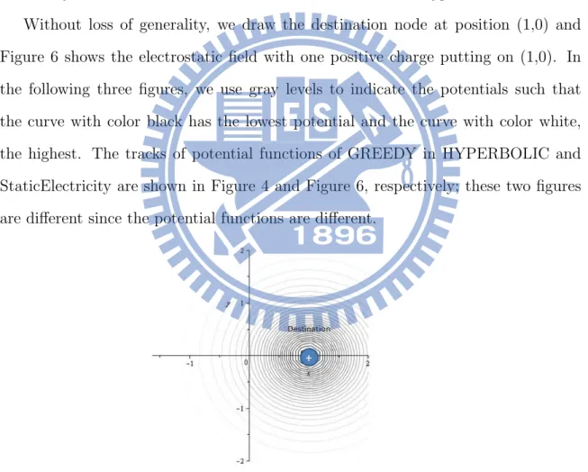
Without loss of generality, we draw the destination node at position (1,0) and Figure 6 shows the electrostatic field with one positive charge putting on (1,0). In the following three figures, we use gray levels to indicate the potentials such that the curve with color black has the lowest potential and the curve with color white, the highest. The tracks of potential functions of GREEDY in HYPERBOLIC and StaticElectricity are shown in Figure 4 and Figure 6, respectively; these two figures are different since the potential functions are different.

Figure 6: The electrostatic field around the destination node.

In Figure 8, we show the situation of one positive charge and two negative charges. Figure 8 shows that when a negative charge occurs, the region closer to the destination node does not change significantly, meaning that if a packet arrives this region, then it will be attracted by the destination node.

Figure 7: the electrostatic field with one positive charge and one negative charge

Figure 8: The electrostatic field with one positive charge and two negative charges.

Algorithm 2 StaticElectricity

Require: The header of the packet (which contains the position information

of the source node, the destination node, MaxStage, CurrentStage, and the list (L) of local minima).

Ensure: A node x∈ N[c] or the packet is discarded.

1: suppose the current node is c and CurrentStage is i;

2: if c is the destination node then the algorithm stops;

3: find the node x∈ N[c] with minimum potential fi(x);

4: if x ̸= c then forward the packet to x;

5: else if i < MaxStage then { i++; put c into L by letting ai = c; goto line 3; }

6: else discard the packet;

4

Experimental results

To perform the simulations, we randomly construct connected UDGs with n nodes in a 100m× 100m area, where n is ranged from 50 to 100, with an increment of 10; for each n, 100 UDGs will be constructed. The transmission range of the UDGs is

r, which will be adjusted so that the average degree d of nodes of is ranged from 4

to 8, with an increment of 0.5. Throughout this section, we assume G is a randomly generated UDG. Let u and v be two distinct nodes in G. Each ordered pair (u, v) will be treated as a pair of the source node and the destination node. To evaluate the performance of a routing algorithm A, we define S to be the set of ordered pairs (u, v) with u̸= v such that A succeeds in exploring a path from u to v. Let |S| denote the cardinality of S. Each of GREEDY, COMPASS, ELLIPSOID, HYPERBOLIC, StaticElectricity, and FACE will run on G.

Again, we use (HYPERBOLIC,MaxStage) to indicate that HYPERBOLIC is used and there are at most MaxStage potential functions. Also, we use (Static-Electricity,MaxStage) to indicate that StaticElectricity is used and there are at most MaxStage potential functions. In our experiment, we run FACE-2 instead of FACE,

which is an improvement of FACE [2]. Notice that if FACE-2 is run on the original UDG (which may not be a planar graph), then the delivery rate may be less than 100%. If FACE-2 is run on GG (Gabriel graph, which is a planar subgraph of thee original UDG), then the delivery rate will be 100%. However, to avoid that FACE-2 will take a long time, we may set up a threshold for the number of hopes in the routing path.

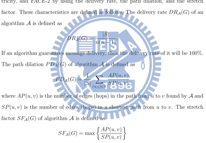
We compare GREEDY, COMPASS, ELLIPSOID, HYPERBOLIC, StaticElec-tricity, and FACE-2 by using the delivery rate, the path dilation, and the stretch factor. These characteristics are defined as follows. The delivery rate DR_A(G) of an algorithm A is defined as

DR_A(G) = |S|

n(n− 1).

If an algorithm guarantees message delivery, then the delivery rate of it will be 100%. The path dilation P D_A(G) of algorithm A is defined as

P D_A(G) = 1 |S| ∑ (u,v)∈S AP (u, v) SP (u, v)

where AP (u, v) is the number of edges (hops) in the path from u to v found byA and

SP (u, v) is the number of edges (hops) in a shortest path from u to v. The stretch

factor SF_A(G) of algorithmA is defined as

SF_A(G) = max {

AP (u, v) SP (u, v)

}

where AP (u, v), SP (u, v), S are defined as above. The path dilation represents the average-case performance of an algorithm and the stretch factor represents the worst-case performance of an algorithm.

Table 1 and also Figure 9 show the delivery rate of GREEDY. These results shows that delivery failure is not uncommon if we use GREEDY, and in sparse graphs, the

delivery rate can be as low as 50%. That is, for these graphs, there are nodes such that half of nodes of the UDG are unreachable if we use GREEDY.

nd 4 4.5 5 5.5 6 6.5 7 7.5 8 50 57.66% 64.70% 71.26% 74.86% 79.84% 84.58% 87.44% 90.96% 94.18% 60 50.42% 57.48% 62.80% 70.53% 76.05% 80.16% 84.21% 88.90% 91.33% 70 47.39% 54.86% 61.53% 69.03% 72.47% 79.94% 83.97% 88.36% 90.79% 80 42.63% 49.99% 56.97% 63.28% 69.66% 75.87% 81.50% 84.32% 87.35% 90 39.14% 46.20% 55.67% 61.82% 67.56% 74.88% 79.51% 83.56% 86.90% 100 37.54% 44.36% 50.73% 55.58% 63.57% 69.36% 75.26% 81.13% 85.22%

Table 1: The delivery rate of GREEDY for UDGs with n nodes and average degree d.

Table 2 compares GREEDY, COMPASS, and ELLIPSOID in terms of their deliv-ery rate and average path dilation. These results show that COMPASS outperforms GREEDY and ELLIPSOID since it has the best delivery rate and its average path dilation is always below 1.10 (i.e., the average path dilation is at most 5-10% greater than the shortest path).

n=50 d=4 d=5 d=6 d=7 d=8 Algorithms DR P D DR P D DR P D DR P D DR P D GREEDY 57.66% 1.0035 71.26% 1.0055 79.84% 1.0069 87.44% 1.0063 94.18% 1.0058 COMPASS 65.42% 1.0503 79.88% 1.0562 86.28% 1.0626 91.70% 1.0674 96.90% 1.0658 ELLIPSOID 50.76% 1.0700 63.40% 1.0844 70.12% 1.0976 77.28% 1.1091 85.38% 1.1146 n=70 d=4 d=5 d=6 d=7 d=8 Algorithms DR P D DR P D DR P D DR P D DR P D GREEDY 47.39% 1.0040 61.53% 1.0066 72.47% 1.0077 83.97% 1.0088 90.79% 1.0086 COMPASS 56.53% 1.0499 70.71% 1.0630 80.56% 1.0722 90.13% 1.0748 94.79% 1.0751 ELLIPSOID 43.50% 1.0657 52.74% 1.0860 62.37% 1.0987 72.96% 1.1137 80.71% 1.1223 n=100 d=4 d=5 d=6 d=7 d=8 Algorithms DR P D DR P D DR P D DR P D DR P D GREEDY 38.73% 1.0057 50.73% 1.0070 63.57% 1.0087 75.26% 1.0108 85.22% 1.0117 COMPASS 47.43% 1.0554 60.02% 1.0682 72.57% 1.0792 83.19% 1.0852 91.39% 1.0900 ELLIPSOID 35.14% 1.0709 43.81% 1.0941 54.34% 1.1121 63.44% 1.1256 72.94% 1.1358

Table 2: The delivery rate (DR) and the average path dilation (P D) of GREEDY, COMPASS and ELLIPSOID for UDGs with n nodes and average degree d.

The trends of Tables 3, 4 and 5 are similar. These tables show the performance of the algorithms under different MaxStage. Table 3 shows the effect of varying

Figure 9: The delivery rate of GREEDY.

MaxStage and average degrees. When the network is sparse (here d = 4), the delivery rate of GREEDY is less than 60%, but the delivery rate of HYPERBOLIC with only one local minimum is more than 80%. Moreover, the delivery rate of HYPERBOLIC is even greater than 95% if MaxStage = 9. Although the average path dilation seems to increases as the MaxStage increases, it is still tolerable. When the network is dense (here d = 8), the delivery rate of GREEDY is greater than 90%, and HYPERBOLIC is icing on the cake. The delivery rate is almost 100% and the average path dilation only about 3.5% longer than the shortest path. Similar behavior can be observed from Tables 4 and 5.

Table 6 compares FACE-2 with GREEDY and our two algorithms HYPERBOLIC and StaticElectricity in terms of delivery rate, average path dilation, and stretch

Figure 10: The delivery rate of GREEDY, COMPASS, and EL-LIPSOID for UDGs with n = 50 nodes.

Figure 11: The delivery rate for GREEDY, COMPASS, and EL-LIPSOID for UDGs with n = 70 nodes.

Figure 12: The delivery rate for GREEDY, COMPASS, and EL-LIPSOID for UDGs with n = 100 nodes.

factor. In this table, “FACE-2 in UDG” means “we run FACE-2 on the original network”, “FACE-2 in GG” means “we run FACE-2 on the Gariel graph of the original graph”. It is no surprising that both the average path dilation and the stretch factor of FACE-2 are much higher than those of the other algorithms. It is surprising that when the network is sparse, the delivery rate of “FACE-2 in UDG” is only 95% even if we allow the threshold to be as large as 2n (2 times the number of nodes of the network), which also means that about 5% of the routing paths take

n=50 d=4 d=5 d=6 d=7 d=8 Algorithms DR P D DR P D DR P D DR P D DR P D GREEDY 57.66% 1.0035 71.26% 1.0055 79.84% 1.0069 87.44% 1.0063 94.18% 1.0058 COMPASS 65.42% 1.0503 79.88% 1.0562 86.28% 1.0626 91.70% 1.0674 96.90% 1.0658 ELLIPSOID 50.76% 1.0700 63.40% 1.0844 70.12% 1.0976 77.28% 1.1091 85.38% 1.1146 (HYPERBOLIC, 1) 80.98% 1.0744 90.68% 1.0600 94.32% 1.0488 96.86% 1.0360 98.94% 1.0209 (HYPERBOLIC, 2) 88.52% 1.1286 94.32% 1.0902 97.04% 1.0689 98.66% 1.0485 99.58% 1.0267 (HYPERBOLIC, 4) 93.40% 1.2028 96.86% 1.1268 98.84% 1.0962 99.56% 1.0642 99.82% 1.0311 (HYPERBOLIC, 9) 96.84% 1.3377 98.80% 1.2158 99.58% 1.1226 99.92% 1.0798 99.94% 1.0358 (StaticElectricity, 1) 70.36% 1.0556 82.92% 1.0497 88.84% 1.0420 94.36% 1.0395 97.88% 1.0243 (StaticElectricity, 2) 75.86% 1.0907 87.98% 1.0900 92.34% 1.0764 96.24% 1.0564 98.80% 1.0337 (StaticElectricity, 4) 82.82% 1.1715 92.18% 1.1450 96.14% 1.1299 98.66% 1.0956 99.68% 1.0493 (StaticElectricity, 9) 90.54% 1.3383 96.76% 1.2590 99.02% 1.1993 99.72% 1.1222 99.88% 1.0548

Table 3: The delivery rate (DR) and the average path dilation (P D) of GREEDY, COMPASS, ELLIPSOID, HYPERBOLIC, and StaticElectricity for UDGs with n = 50 nodes.

n=70 d=4 d=5 d=6 d=7 d=8 Algorithm DR P D DR P D DR P D DR P D DR P D GREEDY 47.39% 1.0040 61.53% 1.0066 72.47% 1.0077 83.97% 1.0088 90.79% 1.0086 COMPASS 56.53% 1.0499 70.71% 1.0630 80.56% 1.0722 90.13% 1.0748 94.79% 1.0751 ELLIPSOID 43.50% 1.0657 52.74% 1.0860 62.37% 1.0987 72.96% 1.1137 80.71% 1.1223 (HYPERBOLIC, 1) 73.81% 1.0936 84.89% 1.0795 90.74% 1.0657 96.11% 1.0446 98.01% 1.0303 (HYPERBOLIC, 2) 82.16% 1.1569 89.91% 1.1206 94.70% 1.0995 97.77% 1.0577 99.17% 1.0400 (HYPERBOLIC, 4) 89.31% 1.2620 94.03% 1.1833 97.49% 1.1398 98.77% 1.1137 99.70% 1.0489 (HYPERBOLIC, 9) 94.21% 1.4882 97.37% 1.3380 99.29% 1.2447 99.61% 1.1214 99.89% 1.0581 (StaticElectricity, 1) 59.16% 1.0543 74.27% 1.0614 83.16% 1.0551 92.09% 1.0464 96.43% 1.0342 (StaticElectricity, 2) 64.61% 1.0964 79.61% 1.1077 87.26% 1.0904 94.44% 1.0684 98.00% 1.0521 (StaticElectricity, 4) 72.51% 1.2040 86.00% 1.1986 92.63% 1.1749 97.01% 1.0728 99.10% 1.0709 (StaticElectricity, 9) 83.70% 1.4498 92.99% 1.3689 97.11% 1.2913 98.84% 1.1619 99.74% 1.0875

Table 4: The delivery rate (DR) and the average path dilation (P D) of GREEDY, COMPASS, ELLIPSOID, HYPERBOLIC, and StaticElectricity for UDGs with n = 70 nodes.

n=100 d=4 d=5 d=6 d=7 d=8 Algorithm DR P D DR P D DR P D DR P D DR P D GREEDY 38.73% 1.0057 50.73% 1.0070 63.57% 1.0087 75.26% 1.0108 85.22% 1.0117 COMPASS 47.43% 1.0554 60.02% 1.0682 72.57% 1.0792 83.19% 1.0852 91.39% 1.0900 ELLIPSOID 35.14% 1.0709 43.81% 1.0941 54.34% 1.1121 63.44% 1.1256 72.94% 1.1358 (HYPERBOLIC, 1) 64.22% 1.0955 77.94% 1.0963 85.66% 1.0778 92.96% 1.0607 96.84% 1.0472 (HYPERBOLIC, 2) 73.72% 1.1710 85.99% 1.1579 91.14% 1.1222 95.91% 1.0876 98.32% 1.0587 (HYPERBOLIC, 4) 82.50% 1.3095 90.83% 1.2358 94.80% 1.1895 97.69% 1.1178 99.05% 1.0708 (HYPERBOLIC, 9) 90.49% 1.6729 95.48% 1.4791 97.31% 1.3190 99.04% 1.1984 99.69% 1.1153 (StaticElectricity, 1) 49.29% 1.0588 63.24% 1.0683 75.29% 1.0654 85.69% 1.0616 92.60% 1.0492 (StaticElectricity, 2) 54.92% 1.1042 69.14% 1.1260 79.91% 1.1106 90.07% 1.1062 95.41% 1.0806 (StaticElectricity, 4) 63.03% 1.2199 77.18% 1.2478 86.37% 1.2158 94.22% 1.1757 97.63% 1.1221 (StaticElectricity, 9) 74.47% 1.4895 87.30% 1.4838 93.90% 1.4153 98.08% 1.2897 99.20% 1.1707

Table 5: The delivery rate (DR) and the average path dilation (P D) of GREEDY, COMPASS, ELLIPSOID, HYPERBOLIC, and StaticElectricity for UDGs with n = 100 nodes.

more than 2n hops to arrive their destination nodes. n=50 d=4 d=6 d=8 Algorithms DR P D SF DR P D SF DR P D SF GREEDY 57.66% 1.0038 1.0698 79.84% 1.0069 1.1727 94.18% 1.0058 1.1625 (HYPERBOLIC, 1) 80.98% 1.0744 1.7987 94.32% 1.0488 1.6636 98.94% 1.0209 1.0243 (HYPERBOLIC, 29) 96.98% 1.3517 5.6921 99.66% 1.1314 3.3137 99.98% 1.0402 1.0607 (StaticElectricity, 1) 70.36% 1.0556 1.7802 88.84% 1.0420 1.7280 97.88% 1.0243 1.5422 (StaticElectricity, 29) 98.92% 1.6886 7.8157 99.84% 1.2381 4.1858 100.0% 1.0607 2.2700 FACE-2 in UDG 95.36% 4.7717 24.868 96.00% 3.7975 22.5879 95.18% 3.0574 20.804 FACE-2 in GG with threshold 95.58% 5.8619 34.157 99.64% 4.8101 29.9250 99.96% 4.2559 27.037 FACE-2 in GG without threshold 100.0% 6.5335 37.563 100.0% 4.8886 30.4660 100.0% 4.2659 27.037

n=70 d=4 d=6 d=8 Algorithms DR P D SF DR P D SF DR P D SF GREEDY 47.39% 1.0040 1.0918 72.47% 1.0077 1.1790 90.79% 1.0086 1.2382 (HYPERBOLIC, 1) 73.81% 1.0936 2.0192 90.74% 1.0657 1.9201 98.01% 1.0303 1.6003 (HYPERBOLIC, 29) 94.93% 1.5369 8.3203 99.44% 1.2624 6.7189 99.94% 1.0649 2.7067 (StaticElectricity, 1) 59.16% 1.0543 1.7249 83.16% 1.0551 1.9479 96.43% 1.0342 1.8097 (StaticElectricity, 29) 95.64% 1.9489 9.2294 99.47% 1.4200 6.8761 99.99% 1.1009 2.9698 FACE-2 in UDG 96.29% 5.7111 38.811 95.79% 4.9922 31.502 93.83% 4.3232 32.830 FACE-2 in GG with threshold 94.19% 6.6834 44.197 99.48% 5.6449 39.687 99.97% 4.6571 34.535 FACE-2 in GG without threshold 100.0% 7.9327 61.731 100.0% 5.7872 41.216 100.0% 4.6763 34.765

n=100 d=4 d=6 d=8 Algorithms DR P D SF DR P D SF DR P D SF GREEDY 38.73% 1.0057 1.1222 63.57% 1.0087 1.2093 85.22% 1.0117 1.2762 (HYPERBOLIC, 1) 64.22% 1.0955 1.9416 85.66% 1.0778 1.9925 96.84% 1.0472 1.8068 (HYPERBOLIC, 29) 92.30% 1.8350 12.934 97.87% 1.3773 9.3820 99.81% 1.1296 4.9085 (StaticElectricity, 1) 49.29% 1.0588 1.8780 75.29% 1.0654 2.0989 92.60% 1.0492 2.1122 (StaticElectricity, 29) 90.59% 2.1443 10.863 98.67% 1.6453 8.9277 99.95% 1.2136 5.4793 FACE-2 in UDG 95.60% 6.5410 46.101 94.75% 6.5071 44.368 92.72% 6.0223 48.371 FACE-2 in GG with threshold 96.30% 7.5630 63.291 99.59% 6.6386 53.299 100.0% 5.3157 43.946 FACE-2 in GG without threshold 100.0% 8.3538 69.627 100.0% 6.7675 55.254 100.0% 5.3157 43.946

Table 6: The delivery rate (DR), average path dilation (P D), and stretch factor (SF ) of GREEDY, HYPERBOLIC, StaticElectricity, and FACE-2.

5

Concluding remarks

The purpose of this thesis is to design two efficient position-based routing algo-rithms for wireless ad hoc networks. Our algoalgo-rithms do not require to run a planariza-tion algorithm in advance. We compare our algorithms to the four famous routing algorithms GREEDY, COMPASS, ELLIPSOID, and FACE in terms of delivery rate, average path dilation, and stretch factor. Experimental results show that our

algo-rithms have very good delivery rate and have small average path dilation and stretch factor.

References

[1] S. Ansari, L. Narayanan, and J. Opatrny, A generalization of the face routing algorithm to a class of non-planar networks, the Second Annual International Conference on Mobile and Ubiquitous Systems: Network-ing and Services (MobiQuitous’05), pp. 213-224, 2005.

[2] P. Bose, P. Morin, I. Stojmenovic, and J. Urrutia, Routing with guar-anteed delivery in ad hoc wireless networks, Wireless Networks 7, pp. 609-616, 2001.

[3] S. Datta, I. Stojenovic, and J. Wu, Internal node and shortcut based routing with guaranteed delivery in wireless networks, Cluster Comput-ing 5, pp. 169-178, 2002.

[4] G.W. Denardin, C.H. Barriquello, A. Campos, and R.N. do Prado, A geographic routing hybrid approach for void resolution in wireless sensor networks, The Journal of Systems and Software 84, pp. 1577-1590, 2011. [5] T. Fevens, A.E. Abdallah, and B.N. Bennani, Randomized AB-face-AB routing algorithms in mobile ad hoc networks, ADHOC-NOW 2005, LNCS 3738, pp. 43-56, 2005.

[6] R. Jain, A. Puri, and R. Sengupta, Geographical routing using partial information for wireless ad hoc networks, IEEE Personal Communica-tions Magazine 8, pp. 48-57, 2001.

[7] E. Kranakis, H. Singh, and J. Urrutia, Compass routing on geometric networks, Proceedings of the 11th Canadian Conference on Computa-tional Geometry 1999.

[8] Y. Li, Y. Yang, and X. Lu, Rules of designing routing metrics for greedy, face, and combined greedy-face routing, IEEE Transactions on Mobile Computing 9(4), pp. 582-595, 2010.

[9] M. Mauve, J. Widmer, and H. Hartenstein, A Survey on Position-Based Routing in Mobile Ad-Hoc Networks, IEEE Network Magazine 15(6), pp. 30-39, 2001.

[10] A.M. Popescu, I.G. Tudorache, B. Peng, and A.H. Kemp, Surveying po-sition based routing protocols for wireless sensor and ad-hoc networks, International Journal of Communication Networks and Information Se-curity 4(1), pp. 41-67, 2012.

[11] L.K. Qabajeh, L.M. Hiah, and M.M. Qabajeh, A qualitative comparison of position-based routing protocols for ad-hoc networks, International Journal of Computer Science and Network Security 9(2), pp. 131-140, 2009.

[12] L. Shu, Y. Zhang, L. Yang, Y. Wang, M. Hauswirth, and N. Xiong, TPGF: geographic routing in wireless multimedia sensor networks, Telecommunication Systems 44, pp. 79-95, 2010.

[13] H. Takagi and L. Kleinrock, Optimal transmission ranges for randomly distributed packet radio terminals, IEEE Transactions on Communica-tions 32(3), pp.246-257, 1984.

[14] S. Tao, A.L. Ananda, and M.C. Chan, Greedy face routing with face identification support in wireless networks, Computer Networks 54, pp. 3431-3448, 2010.

[15] D. B. West, Introduction to Graph Theory, Prentice-Hall, Inc., 2000. [16] K. Yamazaki and K. Sezaki, The proposal of geographical routing

pro-tocols for location-aware services, Electronics and Communications in Japan 87, 2004.