使用時變機率分配之歐式選擇權定價模型研究

全文

(1)國立交通大學資訊管理研究所博. 士. 論. 文. 使用時變機率分配之歐式選擇權定價模型研究 Using Computational Methodology to Price European Options with Time Variant Distributions. 研究生：盛介中指導教授：陳安斌博士. 中華民國. 96. 年. 6. 月.

(2) 使用時變機率分配之歐式選擇權定價模型研究 Using Computational Methodology to Price European Options with Time Variant Distributions 研究生：盛介中. Student: Chieh-Chung Sheng. 指導教授：陳安斌博士. Advisor: An-Pin Chen. 國立交通大學資訊管理研究所博士論文. A Dissertation Submitted to Institute of Information Management College of Management National Chiao Tung University in Partial Fulfillment of the Requirements for the Degree of Doctor of Philosophy in Information Management June 2007 Hsinchu, Taiwan, the Republic of China. 中華民國九十六年六月. 2.

(3) Acknowledgement It takes me five years to accomplish my doctoral degree. And, it may be my last diploma of my entire life. I have to firstly thank my advisor Professor An-Pin Chen, he always supports me and gives me a lot of suggestions. Next, Professor Shrane-Koung Chou first taught me how to apply information technology to solve real world problems during my college time. He is always amiable to students and having abundant knowledge among cross field applications. It is also worth mentioned that Professor Han-Lin Li is a well disciplined scholar having strong logic concepts and theoretical backgrounds. I learned a lot from him about how to be a good scholar and how to perform deliberated research. Apart from my teachers, I have to thank my parents and parents in law who always support me without any reservation. Also, I have to thank my wife Kates Chiu who gives me a lot of supports on research and takes care of my life. It is also worth mentioned that Professor Mu-Yan Chen is one of my best friends who gives me strong supports on discussing research ideas and we exchanges learning experiences with each other. Finally, I thank all my doctoral dissertation committee members. They gave me a lot of suggestions on improving my final dissertation.. 1.

(4) Content 1. Introduction ............................................................................................................................6 2. Backgrounds on option pricing ..............................................................................................8 2.1 Options and fair prices..................................................................................................8 2.2 Risk-neutral distributions ........................................................................................... 11 2.3 Option pricing models ................................................................................................12 2.4 Studies on implied volatility.......................................................................................16 3. Computational approach for pricing European options........................................................17 3.1 Observations regarding actual payoff distributions....................................................18 3.2 Observations regarding implied volatilities................................................................21 3.3 The computational approach ......................................................................................28 3.4 The pricing algorithm .................................................................................................38 3.4.1 The actual distribution generating algorithm...................................................38 3.4.2 The pricing algorithm ......................................................................................40 4. Empirical tests and future studies.........................................................................................42 4.1 Empirical test..............................................................................................................43 4.2 Future studies..............................................................................................................45 5. Conclusions ..........................................................................................................................55 Reference ..................................................................................................................................57. 2.

(5) Graphs Figure 1. Relationship between option values and time to maturity ........................................10 Figure 2. Standard deviations of actual distributions ...............................................................21 Figure 3: Market Expected Possibility Space generated by (FP, Vt) ........................................24 Figure 4: The actual implied volatility distribution map of (FP, IV) compared to the normal distribution, D(µ,σ,skewness,kurtosis) = D(0.0755, 1.1066) ...................................................25 Figure 5: The market implied volatility distribution map of (S, IV) compared to the normal distribution, D’(µ,σ) = D’(0.046030, 1.057034) ......................................................................26 Figure 6. The core concept of the proposed model ..................................................................29 Figure 7. Rotating the factor weights clockwise decreases the mean value of the distribution32 Figure. 8 The transformed distribution after rotated the weighting factors..............................34 Figure 9. Transformed payoff distribution after applying formula (3.15)................................35 Figure 10. 30 days sliding window volatility of TX.................................................................46 Figure 11. Selecting proper sampling period according to volatility change ...........................47 Figure 12. TX index values ......................................................................................................48 Figure 13. Selecting proper sampling period according to current pricesc ..............................48 Figure 14. 50 days payoff distribution with 40 intervals..........................................................50 Figure 15. 50 days payoff distribution with 120 intervals........................................................51 Figure 16. Piecewise linear function concept...........................................................................52 Figure 17. A piecewise linear regression sample......................................................................53 Figure 18. Frequency peak values of different days to maturity ..............................................54. 3.

(6) Tables Table 1 Types of exotic options ..................................................................................................9 Table 2. The actual distribution maps compared to the normal distributions. ..........................18 Table 3: The cumulative possibility distributions .....................................................................26 Table 4. Pricing error.................................................................................................................44. 4.

(7) Using Computational Methodology to Price European Options with Time Variant Distributions. Abstract. Most option pricing methods use mathematical distributions to approximate underlying asset behavior. However, pure mathematical distribution approaches have difficulty approximating the actual distribution. This study first introduces an innovative computational method for pricing European options based on time variant distributions of the underlying asset. The distribution can be either mathematically generated or simply apply real payoff distributions. Moreover, this computational approach can also be applied to applications related to expected value computation that require actual distributions rather than mathematical distributions. This study makes the following contributions: a) solving the risk neutral issue related to price options with none-mathematical distributions; b) proposing a simple method for adjusting standard deviation based on the need to apply short term volatility to real world applications; c) demonstrating option pricing algorithms that are easy to apply to cross field applications; d) helping traders to generate their own distributions to price new derivative instruments without the difficulty of deriving new closed form formulas.. Keywords: Option pricing, actual distribution, expected value, implied volatility. 5.

(8) 1. Introduction. An option is a tradable contract that confers the right, but not the obligation, to buy (call) or sell (put) an underlying asset at an agreed-upon price during a certain period or on a specific date. The value of such a contract is termed the option price or option value. Thus, an option price is the expected return of the underlying asset’s final settlement price larger (call) or lesser (put) than the desired value (the agreed-upon price). Because option value is the expected return of a usually unpredictable underlying asset, option pricing methodologies have been widely adopted by cross fields applications that need to obtain the target’s expected value under uncertainties. For example, the real options analysis (ROA) approach has been widely adopted for assessing information technology investments since the early 1990s [1][2]. Thus, improvements in option pricing methodology can significantly benefit expected value related applications. Option pricing methods have been widely researched since the development of the Black-Scholes model (BS model) in 1973 [3]. Numerous studies have attempted to relax the restrictive assumptions of the BS model by using various methodologies to approximate the real payoff distribution on assets in a risk-neutral manner and thus obtain the fair option price. Although it seems natural to obtain the option price based on real asset payoff distribution, this idea has rarely been implemented because the actual distribution never behaves risk-neutrally. This characteristic limits the adoption of option pricing methodology in certain non-mathematical distribution applications because real world behavior frequently disobeys 6.

(9) mathematical distributions. Furthermore, the time value decreasing speed of an option accelerates considerably (non-linearly) as the maturity date approaches, yielding large pricing error, but high-frequency (time interval less than 1 minute) pricing methodologies have received little attention. This non-linear variation characteristic also limits high frequency applications. For example, applications with time to maturity less than one day are not suitable for traditional option pricing methodologies because its expected value varies significantly as the settlement time approaches. If an option pricing model can remove the above limitations, it will be more applicable not only in finance but also in cross field applications. Accordingly, this study proposes a computational model for pricing European options (whose exercise is only permitted on expiry) using time variant distributions of the underlying asset, and verifies the high-frequency pricing performance based on empirical investigation. Experimental results indicate not only that the proposed method can use actual distribution for pricing options which outperforms the BS model, but also that modern computational methods can be adopted to implement option pricing applications rather than using mathematical distributions via closed form formulas. According to the test results, the proposed model contributes significantly to overcoming the limitations of traditional options pricing models when adopted by numerous cross field applications. For example, researchers must determine whether their target index exhibits geometric Brownian motion with lognormal returns when integrating the BS model (or most option pricing models) to calculate the desired expected values, as Benaroch did in his research on IT investment risks [4]. However, there is no need to justify the target’s distribution when using the proposed computational model. Moreover, traders can generate their own distributions to emulate the real world behaviour of any underlying asset without the help of mathematicians to derive closed form formulas while it is also possible that no closed form formula existed in some situations. 7.

(10) The rest of this paper is organized as follows. Section 2 briefly discusses the traditional option pricing methodologies. Section 3 then discusses observations of asset real payoff distribution and the feasibility of applying the actual distribution map to price European options. The pricing methodology and algorithms are also presented in this section. Next, section 4 conducts an empirical study to verify effectiveness of applying real payoff distribution to price European options with the proposed methodology. Finally, conclusions and future research directions are presented in section 5.. 2. Backgrounds on option pricing. Before constructing option pricing models, it is important to realize basic concepts about option and its fair price, option pricing models, and risk-neutral distributions.. 2.1 Options and fair prices An option is a tradable contract that confers the right, but not the obligation, to buy (call) or sell (put) an underlying asset at an agreed-upon price during a certain period or on a specific date. There are two major types of options existed: plain vanilla option, exotic options. Plain vanilla option is the first generation options, for example, European options and American options. American option allows early exercise which enables an investor executes his privilege before final settlement date. On the contrary, European option does not allow early exercise. Finally, the payoff of a plain vanilla option is determined by the final settlement price of the underlying asset at maturity. Besides plain vanilla options, there are three types of exotic options [5]: 1) path-dependent options, 2) multi-factor options and 3) time-dependent options (illustrated in Table 1). The option price of a path-dependent option is determined by the “path” of the underlying asset 8.

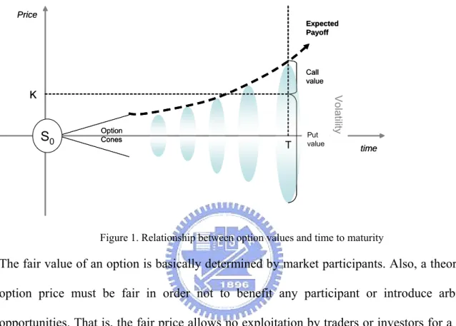
(11) before maturity. The multi-factor option’s price is determined by two or more underlying assets. The time-dependent option determines the price by time and the underlying asset’s current value. Table 1 Types of exotic options Path-dependent options. Multi-factor options. Time-dependent & other options. Average rate option (Asian. Rainbow option. Chooser option. option). Quanto option. Forward start option. Barrier option. Basket option. Binary option. Lookback option. Compound option. Ladder option. Pay-later option. Shout option. Bermudan option. This study focuses on developing a pricing model for European options because it can be modified to price American options. Moreover, cross field applications such as Real Option Analysis (ROA) often apply option pricing models related to European options as well. For a typical European option, the contract is issued with a certain underlying asset to be settled after T days with an agreed upon price K to buy (call) or sell (put) a predetermined amount of the underlying asset. Suppose the current value of the underlying asset is S0, the relationship among put value, call value, time to maturity T, and volatility is demonstrated in Figure 1. For European options, the contract holder must keep the contract until its final settlement day and then evaluate the underlying asset’s price to determine whether the contract should be executed or not. It is obvious that the option price must be determined in a fair manner to deliver an unbiased insight of the contract’s value. Thus, it is important to realize the “fair value” of options. That is the reason why almost all option pricing models 9.

(12) focus on obtaining a theoretical fair price of a certain option to provide traders with a rational basis that can be used to judge whether actual option prices in the marketplace are reasonable, and to help investors determine where to place bids and offers. Price Expected Payoff. Call value. S0. Option Cones. T. Put value. Volatility. K. time. Figure 1. Relationship between option values and time to maturity. The fair value of an option is basically determined by market participants. Also, a theoretical option price must be fair in order not to benefit any participant or introduce arbitrage opportunities. That is, the fair price allows no exploitation by traders or investors for a profit when the option value is efficiently priced by the market [6]. As a result, a fair option price must: a) generate no arbitrage opportunities, b) make no profit for both buyers and writers. a) Generates no arbitrage opportunities: If there is any arbitrage opportunity exists, market participants will execute arbitrage strategies in order to obtain riskless profits. As a result, biased prices will be influenced by investors and no more arbitrage opportunities exist. Thus a fair value must promise no arbitrage opportunities that are widely known as put-call parity. Put-call parity is a strong arbitrage relation first identified by Stoll [7], that between the prices of European put and call options having same underlying with the same strike and expiry, the combinations of options can create positions that are the same as holding the underlying itself. Thus, the call price C, put price P, strike price K and underlying stock price S must satisfy the 10.

(13) following equation: C - P = S - PV(Dividends) - K e(-r T) , where T is the option holding period, r is a continuously compounded interest rate and PV(Dividends) is the present value of the dividends received by the stock owner over the holding period. Although put-call parity identifies the relationship between options and underlying assets, in real world scenario, it is hard to duplicate a stock index with limited stock positions. However, the stock index can be easily duplicated with its relative futures. If there simultaneously exists both options and futures contract of the same underlying asset with the same strike and expiry, put-call parity becomes C - P = FP - PV(Dividends) - K e(-r T) where FP is the futures price of the relative underlying asset. b) Makes no profit for both buyers and writers: If the theoretical option price is always under priced then there will be no option writers selling options with that theoretical value because no one wants to lose money; if the theoretical price is always overpriced then there will be no option buyers purchase that option with theoretical value. A fair option price must also promise an unbiased value that it is equally fair to buy or write an option contract. To sum up, a fair option price guarantees equal profits to all market participants and make no arbitrage opportunities. As a result, every participant in the market will earn only riskless interest rate if the price is fair.. 2.2 Risk-neutral distributions Cox and Ross (1976) established the option price as the expected payoff value discounted at the risk-free interest rate over the risk-neutral distribution of the underlying asset [8]. Nowadays, almost all option pricing models apply risk neutral mathematical distributions to obtain the fair option price. Thus, it is important to realize what a risk neutral distribution is. Risk-neutral means that investors are not risk-averse but instead they do not demand a discounting of the price to take account of risk. With this regard, most option pricing 11.

(14) methodologies estimate the future distribution of the underlying asset in terms of risks, but the pricing models take the average expected price to be the same as holding a riskless bond [9]. The term risk-neutral probability distribution is used to refer to probability distributions which when used as weights in an expected-value calculation will reproduce the market value of financial instruments [10]. Generally speaking, risk-neutral probabilities differ from real-world probabilities because the market price of the underlying asset does not assign value in the same way that a risk-neutral individual would. A risk-neutral distribution must satisfy the following formula [11]: 0 = E(pn – p0) where E(.) denotes the expected value, pn is the future value of the underlying asset, and p0 is the current value of the underlying asset. More practically, if the mean value µ of a payoff distribution equals zero then this distribution is risk-neutral.. 2.3 Option pricing models As discussed before, option price is the expected payoff value discounted at the risk-free interest rate over the risk-neutral distribution of the underlying asset. However, applying none risk-neutral distributions like the real payoff distribution rather than mathematical risk-neutral distributions is difficult because such distributions rarely behaves in a risk-neutral manner. Applying a distribution with non risk-neutral characteristic will violate put-call parity rules [7] because of the arbitrage possibilities associated with the derived put and call prices. This characteristic limits the use of applying practical distribution to price options. Also, a researcher cannot justify if it is worthy to develop closed form formulas to price options with new types of distributions. A simple example is that if a distribution is risk-neutral then the mean value µ must equal zero. However, the µ in a actual distribution rarely equals zero. Another example is that if a researcher wants to integrate 2 or 3 mathematical distributions to 12.

(15) price an option, he may use normal distribution random number generator to produce the simulated distribution space but it does not work because the mean value of randomly generated samples will not be zero. Another example of demonstrating difficulty in applying actual distribution is that it needs different distribution maps for different time to maturity (because this study demonstrates that the actual payoff distribution is time variant, which will be illustrated in the next section). For example, at least n different distribution maps are needed to valuate the option price if it is n days before maturity. Thus, if the sampling data is huge then the pricing speed will be too slow for practical use. Moreover, short-term asset volatility is rarely consistent with that implied by the actual distribution map, leading to significant pricing errors. Consequently, even traders want to apply real asset return distributions, it cannot be practically used to obtain the option price, encouraging researchers to apply mathematically risk-neutral distributions instead. The most classical of these approaches is the BS model, which assumes that the payoff of the underlying asset follows the geometric Brownian motion and has a lognormal distribution with constant volatility and risk-free interest rate before maturity [3]. Since the development of the BS model, more realistic option pricing methodologies have been developed, including: (a) the stochastic interest-rate/volatility option model [12][13][14]; (b) jump-diffusion related models [15][16]; (c) Markovian models [17][18]; and (d) stochastic-volatility jump-diffusion models [19][20]. However, all these models focus on identifying the “right” distributions and pricing options using close form formulas. Consequently, the mathematical distribution never perfectly fits any underlying asset’s actual payoff distribution. Recently, researchers addressed two related empirical phenomena to demonstrate that the real-world distribution do not follow the basic assumption of Black-Scholes model. As a result, researchers forward continuous improvement of pricing methodologies. The first 13.

(16) phenomena is the asymmetric leptokurtic features indicating the return distribution is skewed to the left side and accompanied with a higher peak and two fat tails than those in normal distribution. The second is ‘volatility smile’ which discloses that the implied volatility curve is a convex curve of the strike price while the implied volatility should be constant in Black-Scholes model. In order to deal with the asymmetric leptokurtic features mentioned above, numerous models have been proposed. For example, chaos theory fractal Brownian motion and stable processes [21][22], generalized hyperbolic models[23][24], and time-changed Brownian motions[16][25][22][27]. These models might demonstrate some analytical formulae for standard European call and put options, but they may be unrealistic to obtain analytical solutions for option prices. Meanwhile, different models are also propose to tackle the “volatility smile” in option pricing include: (1) stochastic volatility and ARCH models[28][29][30], (2) constant elasticity model [8][31], (3) normal jump models[12], (4) affine stochastic-volatility and affine jump-diffusion models[32][33][34], (5) implied binomial trees methods[35][36]. These models might not be easy to address analytical solutions for option pricing. Moreover, some of these modes may not solve the asymmetric leptokurtic feature.. Higher Peak Diffusion/Stochastic Models. 50 D a y s P a y of f D istr ibution. Screwed to the left Diffusion/Stochastic Models 4 .0 0. 3 .5 0. 3 .0 0. 2 .5 0. 2 .0 0. Fat Tail Jump Diffusion Models. 1 .5 0. 1 .0 0. 0 .5 0. 0 .0 0 0 .5 6. 0 .4 9. 0 .4 5. 0 .4 0. 0 .3 5. 0 .3 1. 0 .2 6. 14. 0 .2 1. 0 .1 6. 0 .1 2. 0 .0 7. 0 .0 2. - 0 .0 2. - 0 .0 7. - 0 .1 2. - 0 .1 6. - 0 .2 1. - 0 .2 6. - 0 .3 1. - 0 .3 5. Pa yoff R a t e.

(17) In computer science, attempts have also been made to price options using artificial intelligence models to improve options pricing performance. The most popular of these methods is the neural network approach. Unlike classical mathematical methodologies, a neural network is a non-parametric estimation technique which does not make any distributional assumptions regarding the underlying asset. Instead, this approach develops a model using sets of unknown parameters and lets the optimization routine seek the best fitting parameters to obtain the desired results. For example, Hutchinson-Lo-Poggio demonstrated that the neural network approach can be used to price S&P future options [37]. Andrew Carverhill followed this line of research and examined the best method of establishing and train a multi-layer perceptron neural network for option pricing and hedging [38]. Meissner-Kawano also trained neural networks using option prices to address the smiling effect [39] associated with options’ implied volatilities. All these works demonstrate that modern computational theories can offer alternative options pricing methods. In the real world, deriving closed form formulas to price options is time consuming, which decelerates the speed of construction new derivative instruments. Moreover, user may use random number generator to produce a payoff distribution to emulate real assets or simply apply actual distributions instead. However, no solutions for pricing options with user defined distributions existed. Thus, this study focused on determining options price using user defined distributions. Moreover, the proposed model also supports time variant distributions in order to maximize the flexibility of pricing performance. This study also introduces the “real” payoff distribution obtained from a historical sample of Taiwan stock market to demonstrate the proposed model can handle none risk-neutral distributions [58].. 15.

(18) 2.4 Studies on implied volatility In order to observe the real behaviour of an underlying asset, this study introduces a normalization method associated with implied volatility distributions and futures prices. Thus, this section briefly discusses various research topics about implied volatility and future prices. Most financial texts confer that the futures markets aggregate diverse information and expectations regarding the future prices of underlying assets, and thus provide a common reference price which is known as the price discovery function of futures. For example, three topics are commonly discussed in relation to the price discovery function of futures. The first topic deals with the lead-lag relationship and information transmission between the prices of national markets, or between different securities [40][41]. The second topic involves the discussion of volatility spillovers, since volatility is also a source of information [42][43]. The third topic relates to the phenomenon of information transmission between stock index and index futures markets [44][45][46][47]. Similar to futures markets, options markets may also provide a common reference of subsequent real volatility (RV) by calculating the implied volatilities (IV). Early research on the predictive capability of IV found that IV explains variation in future volatilities better than that in historical volatilities (HV). For example, Lantane and Rendleman [48] found that actual option valuations were better explained by actual volatility over the life of the contract than by historical volatility. Chiras and Manaster [49] also tried to compare the predictive power of IV and HV using the CBOE data, and found that IV has superior forecasting power to HV. However, subsequent studies applying time serious methodologies to study the predictive power of implied volatility have yielded mixed results. Some studies have found that IV is a poor method of forecasting subsequent RV, while other studies have found that IV is a good method of forecasting RV. For example, Canina and Figlewski [50] found virtually no relation 16.

(19) between the IV and subsequent RV throughout the remaining life of S&P 100 index options before maturity date. Moreover, Day and Lewis [51] and Lamoureux and Lastrapes [52] both found that GARCH associated with HV is better able to predict RV than IV. Meanwhile, other studies have found that IVs provide reasonably good information on the subsequent RVs of the underlying asset. For example, Harvey and Whaley [53] tested and rejected the hypothesis that volatility changes are unpredictable. Moreover, Fleming [54] examined the performance of the implied volatility of the S&P 100 for forecasting future stock market volatility, and found that although IV has an upward bias but it contains relevant information regarding future volatility.. 3. Computational approach for pricing European. options. This study uses actual distributions to demonstrate the effectiveness of applying the proposed model to price European options. For this reason, this section first discusses observations on actual distributions. Next, this section proposes a computational method of pricing European options with distribution maps saved in databases. In order to prove the effectiveness of the proposed model, this study uses high frequency time interval with one minute time ticks to compute empirical samples. High frequency examples are used to obtain large samples for verification purposes if the execution efficiency of this computation method can feasibly be applied to real world applications. The same concept can also be applied to price European options regardless of time interval.. 17.

(20) 3.1 Observations regarding actual payoff distributions Most option pricing models use mathematical distributions. For example, the BS model assumes that underlying assets follow a geometric Brownian motion with lognormal returns. Meanwhile, other sophisticated option pricing methodologies like the stochastic volatility model apply a flexible distributional structure in which the correlation between volatility shocks and underlying stock returns controls the level of skewness, and use the volatility variation coefficient to control the kurtosis level [19][20]. However, none of these mathematical distributions can precisely describe underlying asset behaviour in the real world. To observe the real behaviour of the underlying assets, this study uses sampling data for the period 01/01/1991 to 09/03/2007 from the Taiwan Stock Exchange Capitalization Weighted Stock Index (TAIEX). Because most mathematical option pricing models discuss the underlying asset return distribution using lognormal related distributions (or with certain modifications), this study calculates the asset return rate as. ln(. Pt ) P0. with different times to. maturity where P0 is the original price and Pt represents the price after t days. The actual distributions are compared with the normal distributions as listed in Table 2.. Table 2. The actual distribution maps compared to the normal distributions. 1. The X-Axis is the nature log asset return rate in % and the Y-Axis is the possibility value in %. 2. The histograms represent the real payoff distribution and the curve lines represent the normal distribution.. 18.

(21) 50 Days Payoff Distribution. 40 Days Payoff Distribution. 4.00. 4.50. 3.50. 4.00. 3.50. 3.00. 3.00. 2.50 2.50. 2.00 2.00. 1.50 1.50. 1.00. 1.00. 0.50. 0.50. 0.00. 0.00 0.51. 0.47. 0.43. 0.38. 0.34. 0.30. 0.26. 0.21. 0.17. 0.13. 0.09. 0.04. 0.00. -0.04. -0.09. -0.13. -0.17. -0.21. -0.26. -0.30. -0.34. 0.56. 0.49. 0.45. 0.40. 0.35. 0.31. 0.26. 0.21. 0.16. 0.12. 0.07. 0.02. -0.02. -0.07. -0.12. -0.16. -0.21. -0.26. -0.31. -0.35. Payoff Rate. Payoff Rate. 30 Days Payoff Distribution. 20 Days Payoff Distribution 7.00. 5.00 4.50. 6.00 4.00 5.00. 3.50 3.00. 4.00. 2.50 3.00. 2.00 1.50. 2.00. 1.00 1.00 0.50 0.00. 0.00 0.37. 0.32. 0.29. 0.26. 0.23. 0.20. 0.17. 0.14. 0.11. 0.08. 0.05. 0.02. -0.02. -0.05. -0.08. -0.11. -0.14. -0.17. -0.20. -0.23. 0.56. 0.47. 0.43. 0.39. 0.34. 0.30. 0.26. 0.22. 0.17. 0.13. 0.09. 0.04. 0.00. -0.04. -0.09. -0.13. -0.17. -0.22. -0.26. -0.30. Payoff Rate. Payoff Rate. 10 Days Payoff Distribution. 1 Days Payoff Distribution. 10.00. 45.00. 9.00. 40.00. 8.00. 35.00. 7.00 30.00 6.00 25.00 5.00 20.00 4.00 15.00 3.00 10.00. 2.00 1.00. 5.00. 0.00. 0.00 0.07. 0.06. 0.05. 0.05. 0.04. 0.03. 0.03. 0.02. 0.01. 0.01. 0.00. -0.01. -0.01. -0.02. -0.03. -0.03. -0.04. -0.05. -0.05. -0.06. -0.07. 0.29. 0.24. 0.21. 0.18. 0.16. 0.13. 0.11. 0.08. 0.05. 0.03. 0.00. -0.03. -0.05. -0.08. -0.11. -0.13. -0.16. -0.20. -0.24. Payoff Rate. Payoff Rate. From Table 2, the real payoff distribution of the asset (TAIEX) varies with days-to-maturity. That is, the actual distribution is time variant. The most interesting finding is that the actual distribution exhibits twin-peak phenomenon in 30, 40 and 50 days to maturity distribution maps. Restated, when days to maturity exceeds 30, the real asset return rate distribution displays two peaks. This twin peak phenomenon has received little attention from academics.. 19.

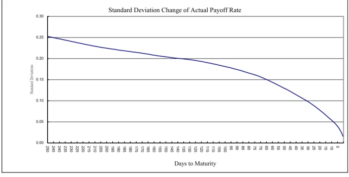
(22) 10 D a y s P a y off D istr ibution. Screwed to the left? Screwed to the right 1 0 .0 0. Higher Peak Still higher. 9 .0 0 8 .0 0 7 .0 0 6 .0 0 5 .0 0 4 .0 0. Fat Tail Not that fat. 3 .0 0 2 .0 0 1 .0 0 0 .0 0. 0 .2 9. 0 .2 4. 0 .2 1. 0 .1 8. 0 .1 6. 0 .1 3. 0 .1 1. 0 .0 8. 0 .0 5. 0 .0 3. 0 .0 0. - 0 .0 3. - 0 .0 5. - 0 .0 8. - 0 .1 1. - 0 .1 3. - 0 .1 6. - 0 .2 0. - 0 .2 4. Pa yoff R a te. The actual distribution clearly shows that mathematical distribution approaches have difficulty obtaining precise option price (at least for the Taiwan stock market), because the actual distribution varies according to time to maturity. The time variant distribution issue limits the use of fixed mathematical distribution pattern across the entire time to maturity range because variation in time to maturity requires the option pricing model to apply time variant distributions. However, it is difficult for mathematical models to apply different distributions for different time to maturity. Furthermore, behavior may differ among assets and markets, so a mathematical model must apply different distributions to maximize its pricing performance for different assets or different markets. Another issue is that the actual payoff distributions, like the time variant distributions with twin peak phenomenon, which are difficult to be described by using mathematical distributions. This issue also limits the cross-field applications of using the traditional option pricing models. Finally, the standard deviation of each distribution map from D1 to D250 is plotted in Figure 2.. 20.

(23) Standard Deviation Change of Actual Payoff Rate 0.30. 0.25. Standard Deviations. 0.20. 0.15. 0.10. 0.05. 0.00 5. 10. 15. 20. 25. 30. 35. 40. 45. 50. 55. 60. 65. 70. 75. 80. 85. 90. 95. 100. 105. 110. 115. 120. 125. 130. 135. 140. 145. 150. 155. 160. 165. 170. 175. 180. 185. 190. 195. 200. 205. 210. 215. 220. 225. 230. 235. 240. 245. 250. Days to Maturity. Figure 2. Standard deviations of actual distributions. 3.2 Observations regarding implied volatilities In order to observe actual payoff behaviors associated with implied volatilities, this study designs a method to demonstrate the relationship between implied volatilities and the underlying asset’s final settlement value. Most researches related to market price observation among various options written on the same underlying asset used to estimate a single volatility with at-the-money or near-the-money options since they are more sensitive to volatility changes and least susceptible to the effect of the bid-ask spread [55]. Beckers [56] and Canina and Figlewski [50] suggests that the option that near the money are better predictors to future real volatility than the IVs of deep in or out of the money options. Thus, this research uses only the daily close price of near-the-money nearby options contract having same underlying with the same strike and expiry for verification. List 1. Notations used in this paper Notations List: C = Call Price 21.

(24) P = Put Price σ = Volatility r = Interest Rate S = Spot Price K = Exercise Price T = Time to Mature in years t = Time to Mature in days N() = Cumulative Standard Normal Distribution Function Nd(μ,σ) = Normal Distribution Function with mean equals μ and standard deviation equalsσ IV = Implied Volatility, yearly Vt = Implied Volatility of t days. FP = Futures Price SP = Final Settlement value. According to Black-Scholes model, the call price C and put price P of a European option can be calculated as follows: C = SN ( d1 ) − Ke − rT N ( d 2 ). (3.1). P = Ke − rT N ( − d 2 ) − SN ( − d1 ). (3.2). d1 =. d2 =. ln(. ln(. S σ2 ) + ( r + )T K 2 σ T. (3.3). S σ2 ) + ( r − )T K 2 σ T. (3.4). This paper modified the calculation method of deriving implied volatility in order to generate an unbiased probability space. Traditionally, computing an implied volatility (IV) requires 22.

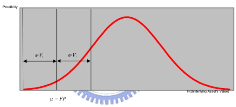
(25) solving (3.1) or (3.2) repeatedly with different trial values for the volatility input. However, the derived IV of a call option (3.1) is rarely equal to the value obtained from a put option (3.2) with the same exercise price and thus most IV related researches use only call or put option into discussions. However, with the relationship indicated in put-call parity, the FP, C and P of the same underlying with the same strike and expiry are tightly coupled with each other that any slight price change of one item will immediately cause the price moves of the other two items. Thus, in order to verify the possibility space formed by FP and IV, this study combines both put and call IVs into a single value IV, namely, the union IV (IVu). Combining (3.1) and (3.2), the IVu can be solved with the following formula: C + P = SN ( d1 ) − Ke − rT N ( d 2 ) + Ke − rT N ( −d 2 ) − SN ( − d1 ). (3.5). Let Oc = {C1, C2, …, Cn} denotes the historical near-the-money call options prices in time interval I, Op = {P1, P2, …, Pn} denotes the historical near-the-money put options prices in I and F = {FP1, FP2, …, FPn} represents the futures prices in I. For the ith historical data in I, using (Ci, Pi, FPi) to generate the ith sampling distribution space and the actual final settlement value of (Ci, Pi) is SPi. Consider the ith historical data in I, take Ci and Pi into (3.5), the yearly IVu of the ith day in I can be solved. Let V = {V1, V2, …, Vn} denotes the IVu in I. Transfer the yearly IVu into days to mature scale, let vt denotes the union implied volatility of t days to mature:. vt =. t × Vi 2 365. (3.6). Suppose SPi and FPi is the relative final settlement value and future price of the ith historical data in I, the actual SP is located at di standard deviations of an Nd(μ,σ) = N(FPi, vt) 23.

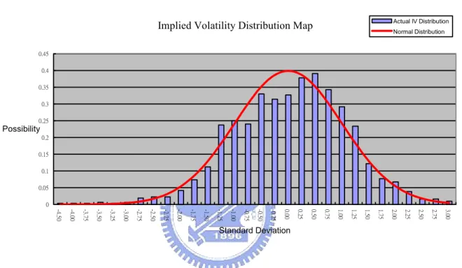
(26) distribution space:. ln( di =. SPi ) FPi vt. (3.7). Thus, for each historical record in I an associated di can be calculated, the collection of di forms a sampling space of standard deviations D = {d1, d2,…, dn}. If the final settlement value follows a normal distribution of Nd(μ,σ) = Nd(FPi, vt), the distribution of D will be a standard normal distribution, Nd(μ,σ) = Nd(0, 1).. Implied Volatility Possibility Space Possibility. σ=Vt. σ= Vt. ln(Underlying Asset's Value). μ = FP. Figure 3: Market Expected Possibility Space generated by (FP, Vt). To observe the behaviors of (FP, IV), this study uses the option and futures prices of Taiwan Stock Exchange Capitalization Weighted Stock Index (TX) from 24/12/2001 to 31/12/2006 in order to testify the results, I=[24/12/2001,31/12/2006]. The risk-less interest rate r applied is monthly fixed deposit interest rate collected from the Central Bank of Taiwan. The calculation results of D are accumulated into Figure 4 in order to compare to normal distribution Nd(0, 1), the (mean, standard deviation) of D is (0.0755, 1.1066) respectively. 24.

(27) Actual IV Distribution. Implied Volatility Distribution Map. Normal Distribution. 0.5 0.45 0.4 0.35 0.3. Possibility0.25 0.2 0.15 0.1 0.05 0 3.25. 3.00. 2.75. 2.50. 2.25. 2.00. 1.75. 1.50. 1.25. 1.00. 0.75. 0.50. 0.25. 0.00. -0.25. -0.50. -0.75. -1.00. -1.25. -1.50. -1.75. -2.00. -2.25. -2.50. -2.75. -3.00. -3.25. -3.50. -3.75. -4.25. -4.50. Standard Deviation. Figure 4: The actual implied volatility distribution map of (FP, IV) compared to the normal distribution, D(µ,σ,skewness,kurtosis) = D(0.0755, 1.1066). Figure 4 exhibits that the distribution of D is roughly similar to Nd(0,1) and is skewed left and peaked compared to Nd(0.0755, 1.1066) but slightly flatter and skewed right compared to Nd(0,1) with thicker tails. In another words, the actual final settlement values of Taiwan Stock Index futures and options roughly follow the behavior of market expectation formed by FP and IV with slightly larger volatilities. Another interesting observation is that there are two possibility peaks located at +0.5 and -0.5 standard deviations. This phenomenon indicates that the final settlement value of the underlying asset tends to bias half an implied volatility in (FP, IV) distributions. Using the close price of stock index instead of the FP in (3.7), this study generates another possibility space formed by IV only. Let D’ = {d’1, d’2,…, d’n}, the (3.7) becomes: SPi ) Si vt. ln( d' i =. (3.8) 25.

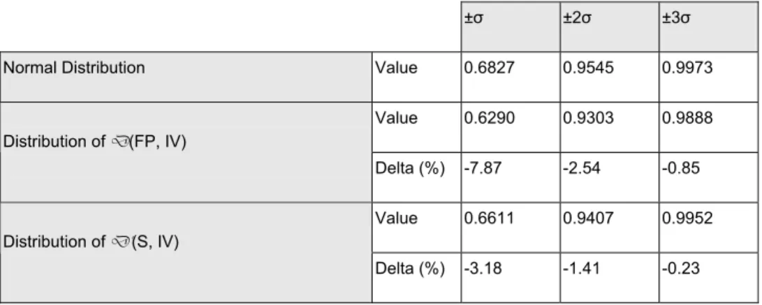
(28) The computed result of D’ in I are summarized into Figure 5. Compared to normal distribution Nd(0, 1), the (mean, standard deviation) of D’ is (0.046030, 1.057034) respectively.. Actual IV Distribution. Implied Volatility Distribution Map. Normal Distribution. 0.45 0.4 0.35 0.3 0.25. Possibility 0.2 0.15 0.1 0.05 0 3.00. 2.75. 2.50. 2.25. 2.00. 1.75. 1.50. 1.25. 1.00. 0.75. 0.50. 0.25. 0.00. -0.25. -0.50. -0.75. -1.00. -1.25. -1.50. -1.75. -2.00. -2.25. -2.50. -2.75. -3.00. -3.25. -3.50. -3.75. -4.00. -4.50. Standard Deviation. Figure 5: The market implied volatility distribution map of (S, IV) compared to the normal distribution, D’(µ,σ) = D’(0.046030, 1.057034). Figure 5 exhibits that the distribution of D’ is more similar to Nd(0,1) than D and is skewed left and peaked compared to Nd(0.046030, 1.057034) but slightly flatter and skewed right compared to Nd(0,1) with thicker tails. Comparing D and D’, the actual final settlement values of Taiwan Stock Index futures and options roughly follow the behavior of the distribution map formed by FP and IV but even closer with the expectation of S and IV. The cumulative possibility distributions from interval ±σ to ±3σ of normal distribution, D and D’ are listed below: Table 3: The cumulative possibility distributions 26.

(29) Normal Distribution. ±σ. ±2σ. ±3σ. Value. 0.6827. 0.9545. 0.9973. Value. 0.6290. 0.9303. 0.9888. Delta (%). -7.87. -2.54. -0.85. Value. 0.6611. 0.9407. 0.9952. Delta (%). -3.18. -1.41. -0.23. Distribution of D(FP, IV). Distribution of D’(S, IV). Table 3 shows that the cumulative possibility of D is smaller than normal distribution about 7.87% in plus minus one standard deviation while 0.85% smaller in ±3σ. D’ is even closer to normal distribution in our testing example, however, both D and D’ clearly indicates that the option price is slightly under estimated. Observing Figure 4, Figure 5 and Table 3, this study concludes that the behavior of TX does not follow normal distributions. However, this conclusion also suggests that an investor can roughly expect the final settlement value of a stock index will locate at the futures price with a standard deviation equals to the implied volatility derived from option price. With this conclusion, investors can expect the price behavior of their stock positions will roughly follow the price behavior of holding both futures and options combinations but most likely having an expectation bias of ±0.5 implied volatilities. Another observation in this research also suggests that (S, IV) combinations are more close to the price behaviors of a stock index than (FP, IV) combinations, that is, applying options only may obtain better risk management performance than using both options and futures combinations. Observing the testing results in section 3.1 and 3.2, this study concludes that the actual behavior of TX does not follow any mathematical distributions. More precisely, it is difficult to approximate an underlying asset like stocks by applying mathematical distribution. 27.

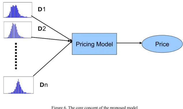
(30) combinations. With this conclusion, this study first introduces the idea to price options with actual distributions.. 3.3 The computational approach Option price is the expected value of the payoff discounted at the risk-free interest rate over the risk-neutral distribution of the underlying asset. Thus, given the price S and an agreed-upon price K for the underlying asset applicable during a certain period T, the option value can be described as follows: C = E(Max(S-K, 0)) P = E(Max(K-S, 0)) Where C denotes the call option price, P represents the put option price, and E(.) is the expected value. In the real world the price of most assets varies continuously, and this variation is described as volatility σ. An option pricing model calculates C or P of the underlying asset under the circumstances (S, K, σ, T, r). The proposed computational model applies actual distribution maps to calculate the desired option price as illustrated in Figure 6.. 28.

(31) D1 D2 Pricing Model. Price. Dn. Figure 6. The core concept of the proposed model. Assume I days of sampling data, with each day containing J time ticks. Then for each sample of ith day and jth time tick Xi,j, the tick payoff rate Ri,j is. Ri , j. ⎧ X i +1,1 − X i , j , if the final settlement price is determined by the opening price on the final settlement day ⎪ X i, j ⎪ =⎨ ⎪ X i +1,n − X i , j , if the final settlement price is determined by the closing price on the final settlement day ⎪ X i, j ⎩. Notably, Ri,j can also be represented as ln((Xi+1,1- Xi,j )/Xi,j) or ln((Xi+1,n- Xi,j )/Xi,j) based on the assumptions of the BS model. However, the difference of applying logarithm or simple payoff rate is minor for high frequency applications. This study avoids unnecessary use of floating point functions to increase execution speed. When using this computational approach to price options, the Ri,j should be modified as:. Ri , j. ⎧ PV ( X i +1,1 − X i , j ) , if the final settlement price is determined by the opening price on the final settlement day ⎪ X i, j ⎪ =⎨ ⎪ PV ( X i +1,n − X i , j ) , if the final settlement price is determined by the closing price on the final settlement day ⎪ X i, j ⎩. where. PV(.) denotes the present value associated with riskless interest rates. Notably, it makes 29.

(32) virtually no difference to calculate PV(.) for less than 50 days to maturity because the impact on interest rates is minor for short term options. The payoff rate can be preprocessed and stored in a database table for further use in achieving a reasonable execution speed when calculating option prices for practical use. Assume an option matures the next day and has strike price S, final settlement price St, exercise price K and current time-tick j. Given m sampling days (which can only generate m-1 sample entries), the call price C can be approximated as follows: m−1. C( S, K , j) = E(max(St − K ,0)) =. ∑. max(S × (1 + Ri , j ) − K ,0). i =1. m −1. Similarly, the Put price P can be approximated as follows: m −1. P ( S , K , j ) = E (max( K − S t ,0)) =. ∑. max( K − S × (1 + Ri , j ),0). i =1. m −1. Consider the riskless interest rate r with time to maturity τ, the Call/Put price can be represented as: m −1. C ( S , K , j , r ,τ ) =. ∑ i =1. m −1 m −1. P ( S , K , j , r ,τ ) =. max(S × (1 + Ri , j ) − e −rτ K ,0). ∑ i =1. (3.9). max(e −rτ K − S × (1 + Ri , j ),0) m −1. (3.10). However, when attempting to determine the option price using (3.9) and (3.10), it quickly becomes obvious that the calculated price does not follow the put-call parity rule because the mean value µ of a actual distribution does not equal zero (implying the actual distribution is not risk-neutral). Notably, arbitraging opportunities occur when the distribution is not risk-neutral. Furthermore, the actual distribution has its own volatility which is difficult to change. For example, if a real payoff distribution is formed based on a ten year period of sample data and 30.

(33) has a standard deviation σ1, but the forecasted volatility of the target option is σ2, then the option must be priced using a distribution with a standard deviation σ2 rather than σ1. If the intrinsic volatility of the actual payoff distribution cannot be transformed to fit the short term volatility, the pricing error will be too large for practical use. Given the difficulty of changing the mean value without influence the variance, this study established a computational method for adjusting both the mean value and variance of an existing distribution to obtain the desired values while maintaining a similar distribution to the original. To obtain risk-neutral characteristics based on the actual distribution, the mean µ of the sampling data must be zero. By observing the actual distribution, if the µ changes from a positive value to zero, the occurrence probability of rightmost (larger) sampling data reduces while the leftmost (smaller) sampling data increases. Based on this phenomenon, a computational method can be developed for adjusting the mean value of the actual distributions by altering the sample occurrence possibilities. The first step is attaching a weighting factor wi to each sampled payoff rate Ri,j. Each wi is assigned an original value 1.0, indicating that it has a “sampling count” of 1. The Call and Put prices thus can be represented as m −1. C ( S , K , j , r ,τ ) =. ∑ i =1. m −1 m −1. P ( S , K , j , r ,τ ) =. max( wi ( S × (1 + Ri , j ' ) − e −rτ K ),0). ∑ i =1. (3.9a). max( wi ( e −rτ K − S × (1 + Ri , j ' )),0) m −1. (3.10a). (Note that Ri,j’ is the standard deviation transformed payoff rate in 3.15) For each set of sampling data, the mean value µ’ and standard deviation σ’ can be calculated as:. 31.

(34) ⎧ ⎪ ⎪µ ' = ⎪ ⎪⎪ ⎨ ⎪ ⎪ ⎪σ ' = ⎪ ⎩⎪. n. ∑R. i, j. i =1. × wi. n. ∑w. i. i =1. n. ∑(R. i, j. i =1. − µ ' ) 2 × wi n. ∑w i =1. i. for the jth tick to maturity. The second step is to adjust the weighting factors to transform the actual distribution into a risk-neutral manner. To achieve this, it is first necessary to sort the sampled payoff rates and position them on the X-axis with weighting factor 1. Assuming that the sample appearance probability changes linearly, the weighting factors can be rotated to modify the distribution, as illustrated in Figure 7. Consequently, by fixing the rotation point to X = 0, the weighting factors can be rotated clockwise to decrease the mean values or anti-clockwise to increase them.. Weighting factor value w = 1.0. Ri,j. 0. Figure 7. Rotating the factor weights clockwise decreases the mean value of the distribution. The weighting factors can be determined by solving the linear equations through the following steps: n. X a = ∑ Ri , j i =1. n. Ri , j ≥ 0. X a 2 = ∑ ( Ri , j ) 2. Ri , j < 0. X b 2 = ∑ ( Ri , j ) 2. i =1. n. Let. X b = ∑ Ri , j i =1. Ri , j ≥ 0. n. and. i =1. Ri , j < 0. (3.11). Let ma denote the slope of the weighting factors for Ri,j ≥ 0, while mb represents the slope of the weighting factors for Ri,j < 0. 32.

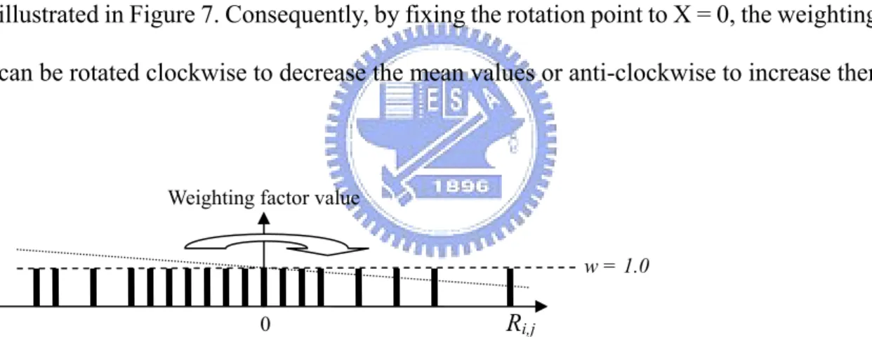
(35) ⎧ X a ma = X b mb ⎪n n ⎨ R ( 1 m R ) Ri , j (1 − mb Ri , j ) = 0 − + ∑ a i, j ⎪∑ i , j i i = 1 = 1 ⎩ Solve (Xa + Xb)Xb ⎧ ⎪ma = X X − X X ⎪ b a2 b2 a ⎨ ⎪mb = ( X a + X b ) X a ⎪ X b X a 2 − X b2 X a Then ⎩. (3.12). Thus, the weighting factor can be transformed as follows:. ⎧1 − ma Ri , j ⎪ wi = ⎨ ⎪⎩1 + mb Ri , j. Rij ≥ 0 Ri , j < 0. (3.13). Combining (3.12) and (3.13) yields the following weighting formula: ⎧ ⎪1 − ⎪ wi = ⎨ ⎪1 + ⎪⎩. (Xa + Xb)Xb Ri , j X b X a 2 − X b2 X a (Xa + Xb)Xa Ri , j X b X a 2 − X b2 X a. Ri , j ≥ 0. Ri , j < 0. (3.14). This computational method can transform any distribution into a risk-neutral distribution while largely preserving the characteristics of the original, as shown in Figure 8.. 33.

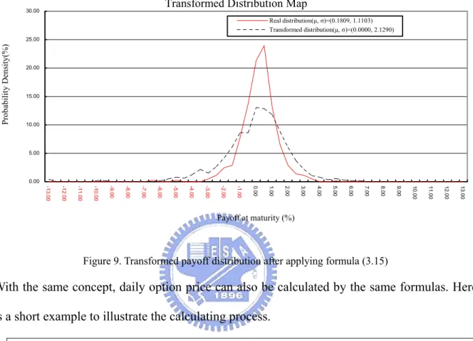
(36) Transformed Distribution Map. 30.00. Real distribution µ = 0.1809 Transformed distribution µ = 0.0000. Probability Density(%). 25.00. 20.00. 15.00. 10.00. 5.00. 0.00 7.00. 6.50. 6.00. 5.50. 5.00. 4.50. 4.00. 3.50. 3.00. 2.50. 2.00. 1.50. 1.00. 0.50. 0.00. -0.50. -1.00. -1.50. -2.00. -2.50. -3.00. -3.50. -4.00. -4.50. -5.00. -5.50. -6.00. -6.50. -7.00. Payoff at maturity (%). Figure. 8 The transformed distribution after rotated the weighting factors. After transforming the actual distribution into a risk-neutral distribution, the next step is to adjust its standard deviation. If the standard deviation after applying formula (3.14) is v, the desired standard deviation of the distribution map is v’; formula (3.14) then can be rewritten as: ⎧ ⎪(1 − ⎪ wi = ⎨ ⎪(1 + ⎪⎩. (Xa + Xb)Xb Ri , j ) Ri , j ≥ 0 X b X a 2 − X b2 X a (Xa + Xb)Xa Ri , j ) Ri , j < 0 X b X a 2 − X b2 X a. and Ri , j ' =. v' × Ri , j v. (3.15). Notably, v’ must be measured using the time to maturity scale (most option pricing applications use annual volatility). Supposing t days (t is a real number) to maturity and anticipated annual volatility is σ, v’ can be estimated by: v' =. t ×σ 2 365. (3.16). Formula (3.15) can transform the actual distribution into the desired volatility without affecting its mean value while maintaining a similar shape to the original distribution. Figure 9 shows the 34.

(37) transformed distribution. The option price thus can be determined via (3.9a), (3.10a), (3.11), (3.15) and (3.16). Transformed Distribution Map. 30.00. Real distribution(µ, σ)=(0.1809, 1.1103) Transformed distribution(µ, σ)=(0.0000, 2.1290). Probability Density(%). 25.00. 20.00. 15.00. 10.00. 5.00. 0.00 13.00. 12.00. 11.00. 10.00. 9.00. 8.00. 7.00. 6.00. 5.00. 4.00. 3.00. 2.00. 1.00. 0.00. -1.00. -2.00. -3.00. -4.00. -5.00. -6.00. -7.00. -8.00. -9.00. -10.00. -11.00. -12.00. -13.00. Payoff at maturity (%). Figure 9. Transformed payoff distribution after applying formula (3.15). With the same concept, daily option price can also be calculated by the same formulas. Here is a short example to illustrate the calculating process. Example 1. Today, suppose TX = 6416. There are 10 days before maturity. The risk-less interest rate = 0.02 and the current call option price on K=6400 is 76. We want to purchase a call option at K = 6400 tomorrow (days to maturity = 9).. Using the following steps to obtain the Call price with the proposed model: z Step1: Selecting desired distribution DT-1 according to time to maturity T z Step2: Using formula (3.14) to adjust selected distribution risk-neutrally z Step3: Using binary search to obtain v’ z Step4: Applying formula (3.14) to obtain the risk-neutral distribution DT 35.

(38) z Step5: Using v’ (in 3.15) to transform distribution DT and apply (3.9a) to get the price. The calculating processes of this example are described as follows: z Step 1: Get distribution map of D10, which can use standard SQL to select the desired. distribution map. SELECT PayoffRate, 1.0 as w FROM DistributionMap WHERE DayCount = 10 z Step 2: Applying (3.14) to adjust the selected distribution risk-neutrally, the weighting. factors are listed below: PayOffRate -1.174731 -0.700737 -0.621213 -0.617936 -0.59823 -0.571291 -0.566551 -0.564137 -0.561379. w 1.647186 1.386052 1.342241 1.340435 1.329579 1.314737 1.312126 1.310796 1.309276. 0.5123461 0.5461306 0.5617606 0.564909 0.5651684 0.6291424 0.7492108 0.8516793. 0.783126 0.768825 0.762209 0.760877 0.760767 0.733687 0.682862 0.639488. •. Step 3: Using binary search to obtain v’ of D10 (applying 3.9a) on D10, v’= 0.1468. 36.

(39) z Step 4: Applying formula (3.14) to obtain the risk-neutral distribution D9. Now, pricing the desired option by D9, select the desired distribution map: SELECT Rat, 1.0 as w FROM DistributionMap WHERE DayCount = 9 Then, applying (3.14) to adjust D9 distribution risk-neutrally. z Step5: Using v’ (in 3.15) to transform distribution D9 and apply (3.9a) to get the. price. Calculate v of D9, v = 0.07; Apply (v’, v) = (0.1468, 0.07) into (3.15) and (3.9a), Call Price = 69.66. In practical use, if a trader or researcher wants to generate a user defined distribution for option pricing, he can use the following steps: Step 1. Choose a random number generator:. Properly choose a random number generator for generating samples. 37.

(40) Step 2. Design distribution maps:. Figure out the desired distribution shape, and then use random generators to produce samples. For example, if a researcher wants to generate a twin peak distribution located at exactly 0.5 and -0.5 stand deviations. He can generate 5,000 samples with Max(N(0.5, 1), 0) and then produce another 5,000 samples with Min(N(-0.5, 1), 0). It is almost sure that the generated distribution map is not risk-neutral because the mean value of the samples does not equal to zero. However, the researcher may safely apply the proposed model to obtain unbiased option values that follows put-call parity. Step 3. Modify distribution maps:. If the researcher does not satisfy with the produced distribution map, he may generate other sampling data and mixes them into the existed distribution maps. For example, if the researcher wants to increase the thickness of the tail at +0.9 standard deviation and -0.9 standard deviation, he may simply generate 50 samples of N(0.9, 1) and N(-0.9, 1) and mixes them with the pre-generated samples.. 3.4 The pricing algorithm The full pricing algorithm comprises two parts. The first part is the algorithm for preparing the distribution map, while the second part is the pricing algorithm.. 3.4.1 The actual distribution generating algorithm. This algorithm is used to generate the actual distribution map to accelerate the calculation process. Because the actual distribution is repeatedly reused for the pricing algorithm, it is optimum to insert new sampling data into the existing distribution maps at the beginning of every trading day (or after trading hours). This algorithm requires minimal execution time if 38.

(41) updates are daily performed. SettlePrice indicates the opening or closing price for the asset (depending on whether the final settlement price is determined based on the opening or closing price on the final settlement day) on the specified date TransactionDate. The sampling data for the previous day are gathered in a data set {TimeTicks, TickPrice} that contains the time tick count and tick price of the underlying asset. The results are stored in the DistributionMap table with the primary index set to (Transaction_date, Time_Ticks). The Transaction_date field represents the sampling date, the Time_Ticks field indicates the time tick counts of the sample, and the Return_Rate field stores the asset return rate.. Algorithm MakeRealDistribution Input: SettlePrice, TransactionDate, {TimeTicks, TickPrice} of previous trading day Output: DistributionMap(Transaction_date, Time_Ticks, Return_Rate) Begin /* Clear old data to prevent duplication */ DELETE FROM DistributionMap WHERE Transaction_date = TransactionDate /* Insert new data */ For Each element pair in {TimeTicks, TickPrice} INSERT INTO DistributionMap (Transaction_date, Time_Ticks, Return_Rate) VALUES (TransactionDate, TimeTicks, SettlePrice/TickPrice) End For End Algorithm. In practical use of the DistributionMap, end users can also write their own programs to generate 39.

(42) any desired mathematical distribution (or combinations) and store the generated samples into the DistributionMap table for the pricing algorithm to calculate the desired option price. For example, a researcher may use two lognormal distributions to simulate the twin-peak distribution as observed for the Taiwan stock market to verify whether it is worthwhile to apply two lognormal distributions to the BS model to improve the pricing performance. Researchers do not need to worry whether the two distribution combinations disobey the risk neutral characteristic before deriving sophisticated mathematical solutions. This characteristic increases the versatility of the pricing algorithm for cross field applications.. 3.4.2 The pricing algorithm. This algorithm is used to price a European option with DistributionMap table generated by MakeRealDistribution. Suppose that the parameter set (S, K, σ, T, r) used to calculate the option price is (SpotPrice, ExercisePrice, Volatility, TimeTicks, RisklessInterestRate), the pricing algorithm can be described as follows:. Algorithm GetOptionPrice Input: SpotPrice, ExercisePrice, Volatility, TimeTicks, RisklessInterestRate, TimeTicks Referenced Table: DistributionMap Output: CallValue, PutValue Begin Define TargetRate = ExcPri/CrnPri – 1 Define TargetMeanVaue = 0 //Suppose that the transformed distribution is //Risk-Neutral. 40.

(43) SELECT Return_Rate, 1.0 as Weight FROM DistributionMap WHERE DistributionMap.Time_Ticks = TimeTicks INTO CURSOR TmpCursor ORDER BY Return_Rate ASC //Generate Weighting Factors. Let Cnt = record counts of TmpCursor. Summation from TmpCursor Let A = ΣReturn_Rate for Return_Rate ≥ 0 Let B = ΣReturn_Rate for Return_Rate <0 Let A2 = Σ(Return_Rate ^2) for Return_Rate ≥ 0 Let B2 = Σ(Return_Rate ^2) for Return_Rate < 0 End Summation. //Formula (3.11). Let OriginalSD = the standard deviation of Weight in TmpCursor Let DaysToMarurity = transfer Timeticks to days to maturity. Let TransformedVolatility = Square Root of (DaysToMaturity*Volatility^2)/365 //Formula (3.16). For Each record in TmpCursor Replace Weight With (TransformedVolatility/OriginalSD) * (1 – (( A + B) * B/( B * A2-A * B2)) * Return_Rate)For Return_Rate ≥ 0 41.

(44) Replace Weight With (TransformedVolatility/OriginalSD) * (1 + (( A + B) * A/( B * A2 - A * B2)) * Return_Rate)For Return_Rate < 0 End For. //Formula (3.15). SELECT SUM(Weight * (SpotPrice * (1 + Return_Rate) - ExercisePrice))/Cnt FROM TmpCursor WHERE TmpCursor.Weight >= TargetRate INTO VARIABLE CallValue. //Formula (3.9a), processed by SQL. SELECT SUM(Weight * (ExercisePrice - SpotPrice * (1 + Return_Rate)))/Cnt ; FROM TmpCur WHERE TmpCursor.Weight < TargetRate INTO VARIABLE PutValue. //Formula (3.10a), processed by SQL. RETURN CallValue, PutValue End Algorithm. The above algorithm is carefully optimized for modern database applications involving SQL syntax and summarizing operations. The elimination of unnecessary floating point functions also increases the execution speed.. 4. Empirical tests and future studies. This session first performs an empirical test and then discusses future studies of the proposed pricing model. 42.

(45) 4.1 Empirical test This study uses tick price data for the period from 03/01/2001 to 17/12/2003 to verify the feasibility of using the proposed computational methods to price TAIEX options using real payoff distributions. There were 270 data recorded for each sampling day, and given the sample data set contained 216,810 entries. Data for the period 03/01/2001 to 31/12/2002 were adopted as the initial distribution map, and pricing errors in high frequency transactions were verified on the last trading day of each month during 2003. The trading hours of the TAIEX run from 9:00 to 13:00. The final settlement price was taken to be the opening price of the final settlement day. The verification procedure is presented below:. Step 1: Generate the initial distribution map.. Filter out incorrect and duplicated data in the database, generate the distribution map using the MakeRealDistribution algorithm, and store it in a database table DistributionMap (Transaction_date, Time_Ticks, Return_Rate) that gives market price data on a per-minute basis between 03/01/2001 and 31/12/2002. Because the trading hours are 9:00 to 13:30, the first minute (9:01) is taken as Time_Ticks = 1 while the last (13:30) is Time_Ticks = 270. The Return_Rate Ri,j equals the tick price of the TAIEX divided by the opening price for the following day: Ri , j =. X i +1,1 X i, j. Step 2: Determine the option price.. This study uses an out-of-sample strategy to verify the pricing performance. The nearest three in-the-money and out-of-the-money call/put option prices were then calculated and priced 43.

(46) using the GetOptionPrice algorithm for every time tick. The same option prices were also calculated using the BS model as a comparison. The riskless interest rate was the monthly fixed deposit interest rate used by the Central Bank of Taiwan.. Step 3: Estimate the pricing efficiency.. The option price is the expected value of St > K for a call option, or St < K for a put option at maturity. Restated, for an ideal call price C = MAX(St – K, 0), the put price should be P = MAX(K – St, 0). Consequently, if an individual spends C dollars to purchase a call option, they should obtain C dollars by holding the option until maturity. The returning ratios Rc and Rp were calculated for each option price to determine the pricing efficiency where the ideal value is 1.0: Rc =. ∑ max(S − K ,0) for call options, and ∑C t. Rp =. ∑ max( K − S ,0) for put options. ∑P t. Table 4 lists the final results. According to the empirical test, the computational method outperforms the traditional BS model in pricing performance.. Table 4. Pricing error. Computational Method. Black-Scholes Method. Call Option, Rc. 0.9290. 0.9037. Pricing Error. 7.10%. 9.63%. Put Option, Rp. 0.9874. 0.9081. Pricing Error. 1.26%. 9.19%. Besides the pricing performance test, the execution speed was tested using Microsoft Visual FoxPro. The computational option model examined in this study is sufficiently efficient to price 44.

(47) 1,000 option prices in 16 seconds (approximately 0.02 seconds each) where the distribution map contains 216,810 sample data, and is run on a 1GB RAM Intel Pentium4 2.6 GHz CPU personal computer system. All analytical results indicate that this computational method provides good pricing performance and efficient execution speeds when run on modern personal computer systems.. 4.2 Future studies Theoretically, pricing options must apply risk-neutral concepts in order to obtain unbiased prices. However, there always exist the needs to price options by user’s personal speculations. This session briefly discusses future studies about determining option pricing via both risk-neutral and none risk-neutral view points. Most option pricing theories suggest the use of risk-neutral distributions to price options. The reason is simple because those models assume that the underlying asset’s price is unpredictable. In another words, if everyone can predict the future price, there will be no one lost money. Because the future price is unpredictable, most pricing models describe the underlying asset’s behavior as “Random Walk”. According to random walk hypothesis, the future price of an underlying asset is independent to its historical price while the future price is dependent only to the current price. For example, if one person tosses a fair coin that he wins 10 dollars if upper side appears or losses 10 dollars if opposite side occurs. If that person owns 100 dollars, the next state he will own either 90 dollars or 110 dollars. That is, the future is unpredictable but the next state is dependant to the current state. For that reason, traditional option pricing theories suggest the use of risk-neutral distributions for option pricing. However, it also lefts a mysterious question: which volatility is correct? Even most option pricing models apply risk-neutral distributions; however, investors have to decide the right 45.

(48) volatility value used for pricing. Thus, investors are bewildered of choosing the correct volatility value for risk-neutral pricing while it is also difficult to select the “right” volatility because it also varies consistently as illustrated in Figure 10.. 30 Days Sliding Window Volatility Change 0.18 0.16 0.14. Volatility. 0.12 0.10 0.08 0.06 0.04 0.02 0.00 2007/2/21. 2006/12/21. 2006/10/21. 2006/8/21. 2006/6/21. 2006/4/21. 2006/2/21. 2005/12/21. 2005/10/21. 2005/8/21. 2005/6/21. 2005/4/21. 2005/2/21. 2004/12/21. 2004/10/21. 2004/8/21. 2004/6/21. 2004/4/21. 2004/2/21. 2003/12/21. 2003/10/21. 2003/8/21. 2003/6/21. 2003/4/21. 2003/2/21. 2002/12/21. 2002/10/21. 2002/8/21. 2002/6/21. 2002/4/21. 2002/2/21. 2001/12/21. 2001/10/21. 2001/8/21. 2001/6/21. 2001/4/21. 2001/2/21. Date. Figure 10. 30 days sliding window volatility of TX. In order to obtain the right volatility used in option pricing models, the most famous methodologies may be ARCH [63] or GARCH [64] approaches. Those methodologies have been proved that they can predict future volatility with an acceptable level [40][65]. For future studies on the proposed computational model, it may combine the use of ARCH or GARCH models to predict future volatilities in order to obtain more accurate prices. Also, artificial intelligence (AI) related models may be applied to forecast future volatilities for obtaining more precise prices with the proposed model. Additionally, the proposed model uses actual distributions instead of mathematical distributions. Thus, it is also feasible to use “proper” periods of sampling data to dynamically construct the desired distribution maps. With this approach, it is possible to use pattern 46.

(49) matching techniques to determine which period of past samples best fits current conditions. And then, uses only properly fitted samples to build up the distribution maps for calculating. To sum up, it is possible to risk-neutrally optimize the proposed model by optimizing forecasted volatilities or sampling periods. For example, if current volatility change looks like the blue area illustrated in Figure 11, users may use pattern matching technique or other methodologies to determine the most similar areas in the past (as in red periods). Using only similar periods as the sampling data, the SQL may be look like: SELECT * FROM DistributionMap WHERE DistributionMap.SamplingDate IN RedPeriod AND DistributionMap.DayCount = DaysToMaturity 30 Days Sliding Window Volatility Change. 0.18. 0.16 0.14. Volatility. 0.12. 0.10 0.08. 0.06. 0.04 0.02. 0.00 2007/2/21. 2006/12/21. 2006/10/21. 2006/8/21. 2006/6/21. 2006/4/21. 2006/2/21. 2005/12/21. 2005/10/21. 2005/8/21. 2005/6/21. 2005/4/21. 2005/2/21. 2004/12/21. 2004/10/21. 2004/8/21. 2004/6/21. 2004/4/21. 2004/2/21. 2003/12/21. 2003/10/21. 2003/8/21. 2003/6/21. 2003/4/21. 2003/2/21. 2002/12/21. 2002/10/21. 2002/8/21. 2002/6/21. 2002/4/21. 2002/2/21. 2001/12/21. 2001/10/21. 2001/8/21. 2001/6/21. 2001/4/21. 2001/2/21. Date. Figure 11. Selecting proper sampling period according to volatility change. Although it is vital for theoretical option pricing models to obey risk-neutral perspectives, it is also equally important for individual investor to have his personal view to the future behavior of the underlying asset. However, if the investor has his own perspective, the derived option prices will not behave risk-neutrally. That is, the put-call parity will be violated if the investor applies his personal views. Figure 12 demonstrates the TX index values from 1/1/2001 to 9/3/2007. It is also clear that the underlying asset’s price behaves differently from volatility 47.

(50) values. TX Index Value 9000.00 8000.00 7000.00 6000.00 5000.00 4000.00 3000.00 2000.00 1000.00 0.00 2007/3/2. 2007/1/2. 2006/11/2. 2006/9/2. 2006/7/2. 2006/5/2. 2006/3/2. 2006/1/2. 2005/11/2. 2005/9/2. 2005/7/2. 2005/5/2. 2005/3/2. 2005/1/2. 2004/11/2. 2004/9/2. 2004/7/2. 2004/5/2. 2004/3/2. 2004/1/2. 2003/11/2. 2003/9/2. 2003/7/2. 2003/5/2. 2003/3/2. 2003/1/2. 2002/11/2. 2002/9/2. 2002/7/2. 2002/5/2. 2002/3/2. 2002/1/2. 2001/11/2. 2001/9/2. 2001/7/2. 2001/5/2. 2001/3/2. 2001/1/2. Date. Figure 12. TX index values. If an investor has his personal viewpoints to the future, it is worth to use pattern matching techniques to decide which interval of the historical period may reflect the future prices. And then, applies the selected samples as the distribution map and turn off the weighting factor rotating mechanism to price the options. However, this methodology cannot provide risk-neutral prices. Taiwan Stock Index 12000 10000 8000 6000 4000. Figure 13. Selecting proper sampling period according to current pricesc 48. 2007/1/3. 2006/1/3. 2005/1/3. 2004/1/3. 2003/1/3. 2002/1/3. 2001/1/3. 2000/1/3. 1999/1/3. 1998/1/3. 1997/1/3. 1996/1/3. 1995/1/3. 1994/1/3. 1993/1/3. 1992/1/3. 0. 1991/1/3. 2000.

(51) For example, current price is marked in blue color as illustrated in Figure 13, users may use pattern matching techniques to determine the most similar periods of the past as the desired distribution map. The SQL command may look like this: SELECT * FROM DistributionMap WHERE DistributionMap.SamplingDate IN RedPeriod AND DistributionMap.DayCount = DaysToMaturity It is also worth mention that applying piecewise linear regression (PLR) methodologies may be applicable for pattern matching. Because PLR uses limited regression lines to describe a certain system characteristics, it is ideal to match different patterns by minimizing mean square errors between different set of PLRs. Here is a simple example to demonstrate the applicable usage of PLR. The observations on actual payoff distributions have been discussed in the previous paragraphs. However, there still lacks detailed analysis. In order to provide in-depth information about the actual distributions, this study applies piecewise linear regression to generalize discrete distributions gathered from historical samples. When observing actual distributions, the distribution is displayed with X-axis represents payoff rate and Y-axis indicates frequency ratio as illustrated in Figure 14.. 49.