科技部補助專題研究計畫成果報告
期末報告
央行獨立性與通貨膨脹
計 畫 類 別 : 個別型計畫 計 畫 編 號 : MOST 104-2410-H-004-009-執 行 期 間 : 104年08月01日至105年09月30日 執 行 單 位 : 國立政治大學經濟學系 計 畫 主 持 人 : 林馨怡 計畫參與人員: 學士級-專任助理人員:張詩雯 碩士班研究生-兼任助理人員:廖珈 碩士班研究生-兼任助理人員:李騏宇 碩士班研究生-兼任助理人員:陳彥凱 報 告 附 件 : 出席國際學術會議心得報告中 華 民 國 105 年 11 月 03 日
中 文 摘 要 : 本文針對追蹤資料分量迴歸模型提出兩階段配適值法,探討央行獨 立性和通貨膨脹之關係。本文有以下貢獻:首先,本文提出之模型 說明央行獨立性的抗通膨效果在通貨膨脹較高時,效果較大,這可 以解釋Franzese (1999) 的理論。其次,本文提出之方法可以解決 用央行總裁更替率當央行獨立性變數的內生性問題。因此,本文能 完整地分析央行獨立性和通膨之關係。 中 文 關 鍵 詞 : 央行獨立性;內生性;通貨膨脹;分量迴歸
英 文 摘 要 : This paper investigates the empirical relationship between central bank independence (CBI) and inflation by proposing a two-stage fitted value approach to a quantile regression for panel data
models. This approach has several advantages. First, Franzese (1999) proposes theoretically that the
anti-inflationary effect of CBI is heterogeneous and is stronger when inflation is higher. Our method,
which estimates the anti-inflationary effect of CBI for various rates of inflation, can expose the conditional heterogeneity of inflation. Second, a simple two-stage approach to the quantile regression for panel data models is proposed to solve the endogeneity problem by using the turnover rate of a central bank governor as a measure of CBI. Third, by exploiting an extensive panel data set, our empirical findings show that the anti-inflationary effect of CBI is stronger in higher
inflation episodes, and is weaker in lower inflation episodes. As we explore this method, the CBI--inflation relationship becomes more convincing.
英 文 關 鍵 詞 : central bank independence; endogeneity; inflation; quantile regression
The Anti-Inflationary Effect of Central Bank
Independence: Heterogeneity and Endogeneity
Abstract
This paper investigates the empirical relationship between central bank inde-pendence (CBI) and inflation by proposing a two-stage fitted value approach to a quantile regression for panel data models. This approach has several advantages. First, Franzese (1999) proposes theoretically that the anti-inflationary effect of CBI is heterogeneous and is stronger when inflation is higher. Our method, which es-timates the anti-inflationary effect of CBI for various rates of inflation, can expose the conditional heterogeneity of inflation. Second, a simple two-stage approach to the quantile regression for panel data models is proposed to solve the endogeneity problem by using the turnover rate of a central bank governor as a measure of CBI. Third, by exploiting an extensive panel data set, our empirical findings show that the anti-inflationary effect of CBI is stronger in higher inflation episodes, and is weaker in lower inflation episodes. As we explore this method, the CBI–inflation relationship becomes more convincing.
JEL classification: E31; E52; E59
1
Introduction
Central bank independence (CBI) refers to the ability of central banks to make de-cisions that are independent of the government. The degree of CBI affects the rates at which the money supply and credit expand, and also has an impact on important aspects of macroeconomic performance. Rogoff (1985) and Lohmann (1992) argue that conservative central bankers attach substantial weight to inflation-rate stabi-lization, and to reducing the inflationary bias resulting from the time-inconsistency problem in their monetary policies. Their theories imply that the effective conser-vativeness or independence of a central bank reduces inflation. Cukierman (1992) also points out that the higher the degree of CBI, the more the monetary author-ity becomes committed to fighting inflation. Thus, independent central banks have been associated with lower inflation rates.
Franzese (1999) constructs a political–economic model where the observed infla-tion is a weighted average of “commitment” inflainfla-tion if the conservative central bank autonomously controls the monetary policy, and “discretionary” inflation if instead the current government controls monetary policy, with the degree of CBI weighting the former. From this model, the anti-inflationary effect of CBI is stronger with higher discretionary inflation relative to commitment inflation. For example, in a high-inflation environment, the political economy imposes substantial inflationary pressure on the government, and the discretionary inflation is higher than the com-mitment inflation. Thus, the anti-inflationary effect of CBI is stronger in situations of higher inflation. On the other hand, if the political economy puts minimal infla-tionary pressure on a government when inflation is low, then the anti-inflainfla-tionary effect of CBI is weaker. Therefore, the anti-inflationary effect of CBI is heteroge-neous at different inflation levels.
The empirical research on the relationship between CBI and inflation is consistent with the theoretical arguments. Alesina (1988, 1989), Grilli, Masciandaro, and Tabellini (1991), Alesina and Summers (1993), and Franzese (1999) find evidence of a negative relationship in developed and industrial countries. Cukierman, Webb, and Neyapti (1992) observe that the legal indicator of CBI is inversely related to inflation in industrial countries, but not in developing countries. They propose that the turnover rate (TOR) of central bank governors is a more appropriate measure of CBI. Because there may be reverse causality running from inflation to the TOR index, Cukierman, Webb, and Neyapti (1992) introduce instrumental variables for TOR to solve the endogeneity problem and find that the effect of CBI on inflation
is negative. Recently, J´acome and V´azquez (2008) and Brumm (2011) have also considered the likely endogeneity of TOR, and affirm the anti-inflationary effects of CBI. Dreher, Sturm, and de Haan (2008) use some political and economic factors as instruments of TOR but find no significant CBI–inflation relationship. In addition, several studies note that the anti-inflationary effect of CBI is influenced by a few influential observations. Temple (1998), de Haan and Kooi (2000), Sturm and de Haan (2001), Bouwman, Jong-A-Pin, and de Haan (2005), Dreher, Sturm, and de Haan (2008), Lin (2010), and Vuletin and Zhu (2011) find that the CBI–inflation relationship is not constant and tends to weaken if high-inflation observations are excluded from the sample. Klomp and de Haan (2010) also confirm empirically that a heterogeneous model is appropriate for estimating the CBI–inflation relationship. Both the theoretical and empirical literature point out that the anti-inflationary effect of CBI is heterogeneous at different inflation levels. Accordingly, our first contribution is to employ a quantile regression for the panel data model to estimate the anti-inflationary effect of CBI at various inflation rates in order to expose the conditional heterogeneity of inflation. The quantile regression ideally uncovers the relationship between CBI and inflation. We include high-inflation observations and explore the implications of both the theory and the data. In addition, the use of TOR leads to endogeneity. Thus, our second contribution is to propose a fitted value approach for the quantile regression for the panel data model to solve for the endogeneity problem that occurs when using TOR as a measure of CBI. The proposed approach is a two-stage estimation procedure. We first obtain the fitted value of the endogenous variable and we then use it to replace the endogenous variable of the model.
Finally, we provide an empirical justification for the relationship between CBI and inflation. In our empirical study, we consider panel data spanning 93 countries over the period 1974–2010. We also include country fixed effects in all specifications to remove the impact on inflation resulting from fixed country characteristics that are potentially correlated with CBI. Our results show that there exists a significantly positive relationship between TOR and inflation at all inflation levels, i.e., a nega-tive CBI–inflation relationship for the whole distribution of inflation. In particular, the anti-inflationary effect of CBI is stronger in high- and middle -inflation episodes than in low-inflation episodes. The empirical results reveal that the CBI–inflation relationship is nonlinear and heterogeneous across different inflation levels, which is consistent with the theoretical argument of Franzese (1999) and several empir-ical studies (Temple, 1998; de Haan and Kooi, 2000; Sturm and de Haan, 2001;
Bouwman, Jong-A-Pin, and de Haan, 2005; Klomp and de Haan, 2010; Vuletin and Zhu, 2011). The results are robust to the inclusion of other inflation-related vari-ables such as openness, the exchange rate regime, political instability, and GDP per capita. We further explore the robustness of the results by using an alternative mea-sure of TOR as well as different classifications of fixed exchange rate regimes. We also consider different unit periods and different sample periods. These robustness checks provide similar trends for the anti-inflationary effect of CBI. Moreover, the effect of the heterogeneity of CBI on inflation is robust to various methods adopted to tackle the problem of endogeneity in relation to TOR.
The remainder of this paper is organized as follows. Section 2 provides the literature review. The econometric methodology and definitions of the data are presented in Section 3. In Section 4, we discuss the results and present the robustness check. In Section 5, we conclude the paper. A list of countries used in this paper is included in the Appendix.
2
Literature Review
As noted by Kydland and Prescott (1977) and Barro and Gordon (1983), the time inconsistency problem of monetary policy leads to inflationary bias. Rogoff (1985) shows that inflationary bias can be reduced by delegating monetary policy to an in-dependent central bank that attaches greater emphasis to inflation rate stabilization than employment stabilization. Rogoff (1985) argues that CBI increases the mon-etary authority’s commitment to fighting inflation, wherein private sector agents reduce their wage increases, thus lowering inflation. Lohmann (1992) proposes that the central banker will implement a nonlinear policy rule and reduce the inflationary bias associated with the time-inconsistency problem of monetary policy. Cukierman (1992) argues that the independence of central banks from their respective political authorities can influence the distribution of inflation. He specifies that a higher de-gree of CBI denotes a stronger commitment on the part of the monetary authority to fight inflation. Therefore, more independent central banks have been associated with lower inflation rates.
Franzese (1999) proposes a political–economic model in which monetary policy is controlled in part by the central bank and in part by the current government; see also Cukierman (2008). The observed inflation is a weighted average of the “com-mitment” inflation if the conservative central bank autonomously controls monetary
policy and “discretionary” inflation if instead the current government controls mon-etary policy, with the degree of CBI weighting the former. From this model, the anti-inflationary effect of CBI is stronger the higher that the discretionary infla-tion would have been relative to what the commitment inflainfla-tion would have been. Franzese (1999) argues that the anti-inflationary effect of CBI is not constant and de-pends on the characteristics of the broader political–economic environment in which the central bank operates. In a high-inflation environment, the political economy exerts great inflationary pressure on the government, and the discretionary inflation is higher than the commitment inflation. Therefore, the anti-inflationary effect of CBI is stronger in cases of higher inflation. On the other hand, the political economy puts little inflationary pressure on the government during times of low inflation, and thus the anti-inflationary effect of CBI is weaker. Franzese (1999) provides theo-retical support to demonstrate that the effect of CBI is heterogeneous and that it varies across levels of inflation.
Empirical work applied to developed and industrial countries supports the neg-ative relationship between CBI and inflation. In considering 16 OECD countries during the period 1973–1985, Alesina (1988) finds that the countries with the most independent central banks have the lowest inflation, whereas those with the most dependent central banks have some of the highest inflation rates. Alesina (1989) obtains similar results for 17 OECD countries during the period 1973–1986. Grilli, Masciandaro, and Tabellini (1991) compare the monetary regimes of 18 OECD coun-tries in the period 1950–1989, and show that lower inflation is associated with higher CBI. In addition, by plotting the cross-country inflation rates for 16 OECD coun-tries against the CBI measure, Alesina and Summers (1993) verify a nearly perfect negative correlation between CBI and inflation during 1955–1988. The empirical results of Franzese (1999) for 18 developed OECD countries in 1972–1990 confirm that the anti-inflationary effect of any given degree of CBI is greater whenever the government has a stronger incentive to pursue inflationary policies.
Cukierman, Webb, and Neyapti (1992) find that the legal indicator of CBI is inversely related to inflation in industrial countries, but not in developing countries, because legal measures of CBI may not reflect the true relationship between CBI and inflation. Cukierman, Webb, and Neyapti (1992) argue that the actual average term in office of a central bank governor may be a better proxy for CBI, and propose using the TOR of central bank governors as an alternative measure of CBI. Of particular note, when using the TOR index as the measure of CBI, it is difficult to determine whether inflation is high because of political interference that leads
to the rapid turnover of central bank officials or because central bank officials are tossed out when they cannot keep inflation low. Cukierman, Webb, and Neyapti (1992) recognize the possibility of endogeneity and introduce instrumental variables for TOR. They find a negative effect of CBI on inflation for 72 countries during the 1950–1989 period. Dreher, Sturm, and de Haan (2008) use the conditional logit model for the likelihood that a central bank governor will be replaced in order to take the endogeneity of TOR into account. They find that the relationship between CBI and inflation is insignificant for 137 countries covering the period 1970–2004. J´acome and V´azquez (2008) explore the effect of CBI on inflation in a sample of 24 Latin American and Caribbean countries during the period 1985–2002. After considering the likely endogeneity of CBI, they find that CBI has a negative effect on inflation. Brumm (2011) addresses the endogeneity of the CBI–inflation relationship by using analysis of covariance structures and finds evidence of a negative relationship for 42 countries during the period from the early 1970s to the mid-1990s.
As noted by several studies, the empirical results of the CBI–inflation relation-ship are affected by a few influential observations (Dreher, Sturm, and de Haan, 2008). Temple (1998) finds that the relationship between CBI and inflation for 18 countries over the 1974–1994 period is extremely sensitive to influential observa-tions, and shows that there exists a negative effect of CBI on inflation in high-income economies. de Haan and Kooi (2000) explore the effect of CBI on inflation in 82 developing countries over the 1980–1989 period, but fail to find any negative effects of CBI. They find that CBI is related to inflation only if high-inflation countries are included in the sample. Sturm and de Haan (2001) extend the data of de Haan and Kooi to include the years 1980–1998 and obtain similar results. Bouwman, Jong-A-Pin, and de Haan (2005) use the quantile regression method to investigate the CBI–inflation relationship in 57 developing countries for the period 1975–1998 and find evidence of a significant relationship only in the higher quantiles of inflation. Lin (2010) revisits the CBI–inflation relationship and shows that the relationship can be positive or negative for different levels of inflation for 44 countries during 1948–1972. Vuletin and Zhu (2011) calculate TOR using a rolling average over the four years that precede a central bank governor change to purge the sample of reverse causality concerns. Their empirical results indicate that the CBI–inflation relationship tends to weaken if the 10% of observations with the highest inflation rates are excluded for 42 countries during the 1972–2006 period.
Most of the existing literature on the CBI–inflation relationship is based on the pooled estimation of panel data, which could provide inconsistent and misleading
estimates for the coefficients of interest. Klomp and de Haan (2010) use a random co-efficient specification of a panel data model to examine to what extent heterogeneity influences the relationship. While they do not find a significant relationship between CBI and inflation for more than 100 countries during the years 1980–2005, they do find evidence of a significant relationship in some developing countries. Klomp and de Haan (2010) thus suggest that a heterogeneous model is the appropriate model for estimating the relationship between CBI and inflation.
3
Econometric Methodology and Data
Our analysis of the effect of CBI on inflation involves an estimation procedure based on the features of quantile regression and panel data models.
3.1
Endogeneity in Panel Data Quantile Regressions
Consider a location-scale shift panel data model, ∀i = 1, · · · , N, t = 1, · · · , T, yit = α1dit+ x0itβ1+ ηi+ (α2dit+ x0itβ2)uit, (1)
where yit is a real-valued dependent variable; dit is an endogenous variable; xit is a
vector of real-valued, continuously distributed, exogenous explanatory variables; ηi
is the parameter that represents the individual fixed effects; α1, α2, β1 and β2 are
unknown parameters; and uit is the error term. The fixed effects ηi in (1) capture
some sources of the variability, or “unobserved heterogeneity,” that is not adequately controlled by other regressors in the model. The fixed effect ηi is a pure location
shift effect. By construction, dit is an endogenous variable and is correlated with
the error term. The aim of this section is to propose a fitted value approach to deal with the endogeneity problem in model (1).
First, consider the following regression model where the endogenous explanatory variable is regressed on the instrumental variable zit:
dit= zit0 γ + vit, (2)
where zit is a vector of the instrumental variable, γ is a (dZ× 1) vector of unknown
parameters, and vit is a real-valued unobserved random variable. Here, zitis allowed
be specified that there is at least one component of zit that is not included in xit.
Replacing dit in (1) by the regression model (2) yields:
yit = α1zit0 γ + x 0
itβ1+ ηi+ α1vit+ α2zit0 γuit+ α2vituit+ x0itβ2uit.
Note that the error terms vit and uit in the above model are independent of the
exogenous explanatory variable xit, and by construction, vit and zit in (2) are
inde-pendent. Assuming that uit is independent of zit, almost surely, we can then obtain
the τ -th conditional quantile function for the above panel data model as follows: Qyit(τ |xit, zit) = α(τ )z 0 itγ + x 0 itβ(τ ) + ηi+ c(τ ), where α(τ ) = α1 + α2Quit(τ ), β(τ ) = β1 + β2Quit(τ ), and c(τ ) = α1Qvit(τ ) +
α2Qvituit(τ ). Note that the fixed effect in our specification does not depend on the
quantile τ , which is more realistic in studying the CBI–inflation relationship. Second, to identify the estimation procedure used, we need to assume that ˆγ is any consistent M-estimator for γ in regression (2). The τ -th conditional quantile function for the panel data model is:
Qyit(τ |xit, zit) = α(τ )z
0 itγ + xˆ
0
itβ(τ ) + ηi+ c(τ ). (3)
The penalized quantile regression approach of Koenker (2004) can then be used to obtain consistent estimators of α(τ ), β(τ ), and c(τ ) in (3), where c(τ ) is viewed as the coefficient of the constant term. This suggests that the parameters of the quantile regression for the panel data model can be estimated by a two-stage procedure. The first stage is to construct a regression of dit on zit and obtain the fitted value zit0 ˆγ.
In the second step, the fitted value zit0 γ is substituted in place of the endogenousˆ variable dit, and the penalized quantile regression approach for panel data models
is used for (3). Therefore, the two-stage estimation corrects for the endogeneity of the quantile regression for the panel data model by replacing dit with zit0γ and canˆ
be viewed as a variant of the fitted value approach.
Several studies propose solving similar endogeneity problems using the quantile regression for panel data models. For example, Arias, Hallock, and Sosa-Escudero (2001), following the control function approach, suggest a two-stage estimation. Harding and Lamarche (2009), Galvao and Montes-Rojas (2010), and Galvao (2011) introduce an instrumental variable quantile regression method for panel data models. However, the former two papers deal with models where the fixed effect depends on the quantile, while the latter two papers consider a dynamic panel data model
without endogenous variables. One of the main contributions of this paper is that it employs a simple two-stage estimation for quantile regressions using a panel data model in which the fixed effect does not depend on the quantile.
3.2
Data
The main data set consists of a panel of 93 countries covering the period 1974–2010 using annual data. A list of constituent countries is provided in the Appendix. Fol-lowing Dreher, Sturm, and de Haan (2008), the dependent variable used in this paper is transformed inflation, and the explanatory variables include TOR, the interaction of TOR and the OECD countries’ dummy, trade openness, a fixed exchange rate regime dummy, political instability, and GDP per capita. Transformed inflation is defined as Πit := (πit/100)/(1 + πit/100), where πit is measured by the annual
change in the consumer price index. Trade openness is measured by the ratio of annual imports plus exports to GDP. The data for inflation, GDP per capita and trade openness are obtained from the World Bank’s World Development Indicators. TOR is measured by the frequency of turnover for central bank governors taken from Dreher, Sturm and de Haan (2008). The fixed exchange rate regime dummy equals one if the exchange rate is classified as fixed according to the de facto classifi-cation of exchange rate regimes in Levy-Yeyati and Sturzenegger (2005), and equals zero otherwise.1 The degree of political instability is measured by the first principal
component of the number of assassinations, strikes, guerrilla warfare attacks, major crises, riots, and revolutions taken from the Databanks International Cross-National Time-Series Data Archive (2012).
The instrumental variables that we take into account for TOR come from Dreher, Sturm, and de Haan (2008); they include elections, lagged inflation, the number of coups, the percentage of veto players who drop, and the average share of the legal term in office that has elapsed. The number of coups includes both successful and unsuccessful attempts to overthrow the government (see Powell and Thyne, 2011). The variable percentage of veto players who drop counts the percentage of veto players who drop from the government in a given year and is taken from data
1The original data of Levy-Yeyati and Sturzenegger (2005) are updated to 2004. To increase the
data availability, we follow the methodology provided by Levy-Yeyati and Sturzenegger in order to construct three classification variables, namely, exchange rate volatility, the volatility of exchange rate changes, and the volatility of reserves, and then identify the de facto exchange rate regime by a K-means cluster analysis.
provided by Beck et al. (2001). The election variable measures the post-election period by the part of the year which is within 12 months after a national election. The average share of the legal term in office that has elapsed is the ratio between the actual and legal duration of a governor’s term in office taken from Dreher, Sturm and de Haan (2008). If the governor’s legal term in office is indefinite or unknown, the term is specified as eight years. All data are updated to 2010.
Table 1 provides basic summary statistics of the data. In panel (A) of Table 1, the median and the third quartile are 7.99% and 14.99%, respectively. However, the mean of inflation is 38.85%, which is much larger than the third quartile of infla-tion. Clearly, the distribution of inflation is right-skewed and the mean is sensitive to extremely large values. While the estimation result of the mean regression for the panel data model is sensitive to the extremely large values of inflation, the quan-tile regression estimation results are robust to extreme values. For the explanatory variables, the average TOR is 0.21, which implies a change of central bank governor every four years and nine months on average. Openness has a symmetric distribu-tion, because its mean and median are close. The average fixed exchange rate regime dummy is 0.43, which means that about 43% of the sample observations are subject to a fixed exchange rate regime. The distributions of political instability and GDP per capita are both right-skewed. Furthermore, all three quantiles of the number of coups, and the percentage of veto players who drop are equal to 0, which is smaller than their averages (0.04, and 0.13, respectively). This shows that at least 75% of their values are at the same level (0) and the averages are sensitive to extremely large values.
The variables in panels (B) and (C) have similar statistical properties to those in panel (A). In particular, inflation, openness, and GDP per capita during 1980–2010 are more volatile than during 1990–2010. The TOR, political instability, and coup variables tend to be lower in value and more stable after 1990, which demonstrates that the political environment is more stable. As the higher TOR of central bank governors is indicative of a lower level of CBI, we can see that the independence of central banks increases after 1990. The characteristics of the remaining variables result in no clear distinction between the periods 1980–2010 and 1990–2010.
4
Empirical Results
4.1
Benchmark Results
Following the theoretical argument of Franzese (1999), the effect of CBI on in-flation is heterogeneous at different inin-flation levels. To account for the varying anti-inflationary impact of CBI at different inflation levels, we investigate the rela-tionship between inflation and CBI in a panel quantile model. As discussed in the Introduction and Section 3, the model captures the CBI–inflation relationship of interest, controls for unobserved individual heterogeneity, and reveals the heteroge-neous effects of regressors on the dependent variable.
To fully investigate the relationship between CBI and inflation, we consider sev-eral inflation-related variables. First, because TOR may not be a good indicator of CBI in industrial countries (Cukierman, Webb, and Neyapti, 1992; Dreher, Sturm and de Haan, 2008), we add to the model not only TOR but also its interaction with an OECD dummy, which is one if a country is developed and zero other-wise. Second, Romer (1993) argues that trade openness is negatively related to inflation because the time inconsistency problem of a given monetary policy is less critical in more open countries. Third, Edwards and Losada (1994), Ghosh et al. (1997) and Calvo and V´egh (1999) all point out that an announced policy of a fixed exchange rate regime may serve as a commitment technology preventing the govern-ment from subsequent temptations to follow expansionary macroeconomic policies and thus lowers inflation. Moreover, Cukierman, Edwards, and Tabellini (1992) propose that countries with more unstable and polarized political systems will have less efficient tax structures, and will thus collect a larger fraction of their revenues through seigniorage. Thus, political instability is considered in the analysis. Finally, economic growth is also an important inflation-related factor, and the growth rate of real GDP per capita is considered as an additional control variable. We use the logarithmic form of the growth rate of real GDP per capita.
When we use TOR as a proxy for CBI to measure its impact on inflation, there may be a reverse causality that runs from inflation to turnover (Cukierman, Webb, and Neyapti, 1992). Such causality leads to endogenous bias in the estimation. Therefore, we take into account the endogeneity problem when examining the CBI– inflation relationship. In this paper, to deal with the endogeneity and heterogeneity, we employ a fitted value approach for the quantile regression for the panel data model using a two-stage estimation procedure. For comparison purposes, we
con-sidered two-stage least squares estimation as well as within estimation for the tra-ditional mean regression using the panel data with endogeneity. Table 2 reports the estimation results of the mean and quantile regressions for the panel data.2 Table 2 shows that the mean and quantile regression estimates of TOR on inflation are all positive. As a higher TOR represents a lower CBI, the empirical results indicate that CBI is anti-inflationary. The results are in line with most empirical studies as well as the theoretical studies of Rogoff (1985), Lohmann (1992), and Cukierman (1992).
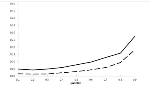
Moreover, the coefficients of TOR on inflation are plotted in Figure 1. In the figure, the horizontal and vertical axes correspondingly denote the quantile and the coefficients of TOR on inflation. The black solid line depicts the quantile regres-sion estimates, and the gray dotted lines represent their 95% confidence intervals. The black dashed line represents the mean regression estimates. Figure 1 shows that the impact of CBI on inflation has a clear trend. The quantile regression esti-mates of TOR increase monotonically, along with the quantiles, in magnitude and significance. That is, the anti-inflationary effects of CBI on inflation are stronger at high and middle quantiles of inflation, whereas they are smaller at low quantiles of inflation. As we review the empirical findings, we see that the CBI–inflation relationship is heterogeneous at different inflation levels. Our results coincide with those of previous empirical studies, and ideally justify the theoretical argument of Franzese (1999), which states that the CBI–inflation relationship tends to weaken if high-inflation observations are excluded. See Temple (1998), de Haan and Kooi (2000), Sturm and de Haan (2001), Bouwman, Jong-A-Pin, and de Haan (2005) and Vuletin and Zhu (2011).
When we examine the interaction of TOR and the OECD dummy, both the mean and quantile regression estimates are negative for all quantiles except for the 0.1 and 0.2 quantiles. These results show that the impact of CBI on inflation is weaker in OECD countries than in non-OECD countries, which indicates that OECD countries have ways of overcoming the dynamic inconsistency problem. One interesting finding
2The adjusted t-statistics of the Levin, Lin and Chu (2002) (LLC) test for inflation, lagged
inflation, openness, and GDP per capita are -9.14, -9.04, -1.37, and -1.8, respectively. The adjusted t-statistics of the Im, Pesaran, and Shin (2003) (IPS) test are -11.88, -13.07, -1.27, and 7.13, respectively. As we cannot reject the hypothesis that openness and GDP per capita have a unit root, we thus first-difference these variables and use them as our regressors. Both tests reject the hypothesis that the first difference of openness has a unit root, which is the same as the result for GDP per capita.
is that the estimates of TOR on inflation are homogeneous across quantiles in OECD countries and are heterogeneous across quantiles in non-OECD countries. In terms of other inflation-related variables, first, the estimates of openness are insignificantly positive, which is not consistent with Romer (1993). Second, the exchange rate is an important factor related to inflation. Many countries have used a fixed exchange rate regime as a nominal anchor for lowering inflation. The quantile regression estimates of the fixed exchange rate regime dummy are negative along with the quantiles both in values and in significance. Here we see that the adoption of a fixed exchange rate regime is much more effective against inflation in higher inflation episodes, and this finding is in line with the findings of Edwards and Losada (1994), Ghosh et al. (1997) and Calvo and V´egh (1999). Third, the mean and quantile regression estimates of political instability are positive, which shows that political instability is an inflationary factor; see also Cukierman, Edwards, and Tabellini (1992), and Dreher, Sturm and de Haan (2008). Finally, the estimates of the growth of real GDP per capita are all negative and they decrease monotonically along with the quantiles. The negative relationship is also supported by Dreher, Sturm and de Haan (2008), but not by Sturm and de Haan (2001).
4.2
Robustness Check
Following Dreher, Sturm and de Haan (2008), we define a new measure for TOR, which equals one if the central bank governor was replaced in a particular year and country, and zero otherwise. Panel (I) in Table 3 reports TOR estimates with the new TOR dummy variable. The quantile regression estimates of the effect of TOR on inflation are positive and increase along with the quantiles. In particular, the TOR estimates are insignificant at the 0.1–0.3 quantiles, significant at the 5% level at the 0.4 quantile, and significant at the 1% level at the 0.5–0.9 quantiles. The empirical results show that the anti-inflationary effect of CBI is heterogeneous at different inflation levels, and is robust with respect to different measures of TOR. However, the results of the interaction of TOR and the OECD dummy are mixed; this may be because TOR is a good proxy for CBI in developing countries, but not in developed countries (Cukierman, Webb, and Neyapti, 1992).
As an additional test, following Vuletin and Zhu (2011), we use the fixed exchange rate regime based on the classification of Reinhart and Rogoff (2004) (henceforth the RR classification) in the model.3 Reinhart and Rogoff (2004) classify exchange
http://www.carmenreinhart.com/research/publications-by-rate regimes into 14 categories and we define the fixed exchange http://www.carmenreinhart.com/research/publications-by-rate regime dummy as one if the RR classification lies between 1 and 4, and zero otherwise. Panel (II) in Table 3 shows the estimates of TOR with the RR classification for the fixed exchange rate regime dummy used. According to the results, the quantile regression estimates of TOR are also positive and increase along with the quantiles. Thus, the CBI–inflation relationship is robust to different classifications of exchange rate regimes.
Dreher, Sturm and de Haan (2008) and Arnone et al. (2007) use data based on five-year averages, and Cukierman, Webb, and Neyapti (1992) use data based on 10-year averages. This paper uses an annual panel model instead of a panel with five-year averages. To provide a better comparison, we transform the annual data into five-year and 10-year averages, and check the robustness of our results. As shown in panels (III) and (IV) in Table 3, the quantile regression estimates of TOR increase monotonically along with the quantiles, are statistically significant at the 0.3–0.9 quantiles for the data transformed into five-year averages, and are statistically significant at the 0.6–0.9 quantiles for the data transformed into 10-year averages. The anti-inflationary effect of CBI on inflation is heterogeneous at different levels of inflation. By using one-year, five-year, and 10-year averages, we allow for actual independence and changes in institutional characteristics (Vuletin and Zhu, 2011). Therefore, our results are robust with respect to different unit periods and moderate institutional change.
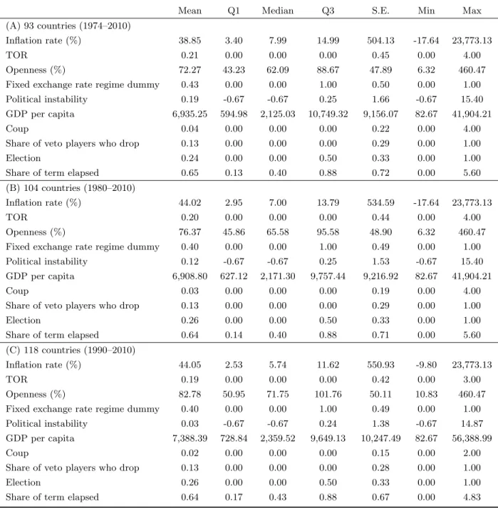
Finally, we consider different sample periods of the data. Figure 2 plots the quantile regression estimates of TOR on inflation over the periods 1980–2010 and 1990–2010. The solid line represents estimates of the data during 1980–2010, and the dashed line represents estimates of the data during 1990–2010. We find that the anti-inflationary effect of CBI is stronger in middle- and high-inflation episodes and weaker in low-inflation episodes, which confirms the robustness of our results. Furthermore, Franzese (1999) finds that several anti-inflationary factors, such as trade openness and the strength of the financial sector, become stronger and more stable with time, and CBI plays a less important role in restraining inflation. Fig-ure 2 shows that the anti-inflationary effects of CBI during 1990–2010 are lower than those during 1980–2010, which is consistent with the findings of Franzese (1999).
4.3
The Endogeneity of TOR
We use instrumental variables for the endogeneity problem of TOR. As described before, the average share of the legal term in office that has elapsed is the ratio between the actual and legal duration of a governor’s term in office. If the legal term in office of a governor is indefinite or unknown, then the term is specified as the maximum, which is eight years. Following Dreher, Sturm and de Haan (2008), two alternatives of the legal term are (1) the average term in office in the whole sample, and (2) the average legal term in those countries where central bank law specifies a governor’s term in office. The former is 3.7 years and the latter is five years. Panels (I) and (II) in Table 4 present TOR estimates with the two alternatives being used. Both panels show that the regression estimates of TOR on inflation are significant in middle- and high-inflation episodes and insignificant in low-inflation episodes. CBI remains more anti-inflationary as inflation becomes higher.
Instead of using instrumental variables to solve the endogeneity problem, Klomp and de Haan (2010) and Vuletin and Zhu (2011) employ a rolling average of TOR over the preceding years to replace the current TOR. Using this method, we do not include current or future turnovers of central bank governors in the calculation of the current value of TOR, so that we avoid reverse causality concerns. We follow Klomp and de Haan (2010) and Vuletin and Zhu (2011) and set the length of the windows equal to four years. Without using the instrumental variable method, we use Koenker’s (2004) ordinary quantile regression for the panel data model and within estimation. Panel (III) in Table 4 reports the estimates of TOR and shows that the quantile regression estimates of TOR are positive and increase along with the quantiles. The results are similar to the benchmark results. Thus, the CBI– inflation relationship is robust to various methods used to deal with the endogeneity problem.
5
Conclusions
This paper proposed a fitted value approach to quantile regressions for panel data models to examine the CBI–inflation relationship. With this we attempted to solve the possible endogeneity problem by using the TOR index as a measure of CBI. The econometric method proposed in this paper demonstrates a fruitfully exploitable al-ternative compromise. Moreover, both the theoretical and empirical literature point out that the anti-inflationary effect of CBI is heterogeneous at different inflation
lev-els. By exploiting an extensive panel data set, the findings in this paper imply that CBI is more anti-inflationary in cases of higher inflation rates. This paper provided an empirical justification for the heterogeneous anti-inflationary characteristics of CBI. The relationship between CBI and inflation becomes more convincing when the panel quantile model with a fitted value approach is used.
References
Alesina, Alberto. (1988) “Macroeconomics and Politics.” NBER Macroeconomics Annual, 3, 13–52.
Alesina, Alberto. (1989) “Politics and Business Cycles in Industrial Democracies.” Economic Policy, 8, 55–98.
Alesina, Alberto, and Lawrence H. Summers. (1993) “Central Bank Independence and Macroeconomic Performance: Some Comparative Evidence.” Journal of Money, Credit and Banking, 25, 151–62.
Arias, Omar, Kevin F. Hallock, and Walter Sosa-Escudero. (2001) “Individual Het-erogeneity in the Returns to Schooling: Instrumental Variables Quantile Re-gression Using Twins Data.” Empirical Economics, 26, 7–40.
Arnone, Marco, Bernard J. Laurens, Jean-Fran¸cois Segalotto, and Martin Sommer. (2007) “Central Bank Autonomy: Lessons from Global Trends.” IMF Working Paper, No. 07/88.
Barro, Robert J., and David B. Gordon. (1983) “A Positive Theory of Monetary Policy in the Natural Rate Model?” Journal of Political Economy, 91, 589–610. Beck, Thorsten, George Clarke, Alberto Groff, Philip Keefer, and Patrick Walsh. (2001) “New Tools in Comparative Political Economy: The Database of Po-litical Institutions.” World Bank Economic Review, 15, 165–76.
Bouwman, Kees, Richard Jong-A-Pin, and Jakob de Haan. (2005) “On the Rela-tionship Between Central Bank Independence and Inflation: Some More Bad News.” Applied Financial Economics Letters, 1, 381–85.
Brumm, Harold J. (2011) “Inflation and Central Bank Independence: Two-Way Causality?” Economics Letters, 111, 220–22.
Calvo, Guillermo A., and Carlos A. V´egh. (1999) “Inflation Stabilization and BOP Crises in Developing Countries.” In Handbook of Macroeconomics, Vol. C, edited by J. B. Taylor, and Michael Woodford, pp. 1531–614. Amsterdam: Elsevier Science, North Holland.
Cukierman, Alex. (1992) Central Bank Strategy, Credibility, and Independence: Theory and Evidence. Cambridge, MA: MIT Press.
Cukierman, Alex. (2008) “Central Bank Independence and Monetary Policymak-ing Institutions — Past, Present and Future.” European Journal of Political Economy, 24, 722–36.
Cukierman, Alex, Sebastian Edwards, and Guido Tabellini. (1992) “Seigniorage and Political Instability.” American Economic Review, 82, 537–55.
Cukierman, Alex, Steven B. Webb, and Bilin Neyapti. (1992) “Measuring the Inde-pendence of Central Banks and Its Effect on Policy Outcomes.” World Bank Economic Review, 6, 353–98.
de Haan, Jakob, and Willem J. Kooi. (2000) “Does Central Bank Independence Re-ally Matter? New Evidence for Developing Countries Using a New Indicator.” Journal of Banking and Finance, 24, 643–64.
Dreher, Axel, Jan-Egbert Sturm, and Jakob de Haan. (2008) “Does High Inflation Cause Central Bankers to Lose Their Job? Evidence Based on a New Data Set.” European Journal of Political Economy, 24, 778–87.
Edwards, Sebastian, and Fernando J. Losada. (1994) “Fixed Exchange Rates, In-flation and Macroeconomic Discipline.” NBER Working Paper No. 4661. Robert J. Franzese. (1999) “Partially Independent Central Banks, Politically
Re-sponsive Governments, and Inflation.” American Journal of Political Science, 43, 681–706.
Galvao, Antonio F. (2011) “Quantile Regression for Dynamic Panel Data with Fixed Effects.” Journal of Econometrics, 164, 142–57.
Galvao, Antonio F., and Gabriel V. Montes-Rojas. (2010) “Penalized Quantile Regression for Dynamic Panel Data.” Journal of Statistical Planning and Inference, 140, 3476–97.
Ghosh, Atish R., Anne-Marie Gulde, Jonathan D. Ostry, and Holger C. Wolf. (1997) “Does the Nominal Exchange Rate Regime Matter?” NBER Working Paper No. 5874.
Grilli, Vittorio, Donato Masciandaro, and Guido Tabellini. (1991) “Political and Monetary Institutions and Public Financial Policies in the Industrial Coun-tries.” Economic Policy, 6, 341–92.
for Estimating Panel Data Models Using Instrumental Variables.” Economics Letters, 104, 133–35.
Im, Kyung So, M.Hashem Pesaran, and Yongcheol Shin. (2003) “Testing for Unit Roots in Heterogeneous Panels.” Journal of Econometrics, 115, 53–74.
J´acome, Luis I., and Francisco V´azquez. (2008) “Is There any Link between Legal Central Bank Independence and Inflation? Evidence from Latin America and the Caribbean.” European Journal of Political Economy, 24, 788–801.
Klomp, Jeroen, and Jakob de Haan. (2010) “Central Bank Independence and Infla-tion Revisited.” Public Choice, 144, 445–57.
Koenker, Roger. (2004) “Quantile Regression for Longitudinal Data.” Journal of Multivariate Analysis, 91, 74–89.
Kydland, Finn E., and Edward C. Prescott. (1977) “Rules Rather than Discretion: The Inconsistency of Optimal Plans.” Journal of Political Economy, 85, 473– 92.
Levy-Yeyati, Eduardo, and Federico Sturzenegger. (2005) “Classifying Exchange Rate Regimes: Deeds vs. Words.” European Economic Review, 49, 1603–35. Levin, Andrew, Chien-Fu Lin, and Chia-Shang James Chu. (2002) “Unit Root
Tests in Panel Data: Asymptotic and Finite-Sample Properties.” Journal of Econometrics, 108, 1–24.
Lin, Hsin-Yi. (2010) “A Revisit of the Relation Between Central Bank Independence and Inflation.” The Empirical Economics Letters, 9, 139–43.
Lohmann, Susanne. (1992) “Optimal Commitment in Monetary Policy: Credibility versus Flexibility.” American Economic Review, 82, 273–86.
Powell, Jonathan M., and Clayton L. Thyne. (2011) “Global Instances of Coups From 1950 to 2010: A New Dataset.” Journal of Peace Research, 48, 249–59. Reinhart, Carmen M., and Kenneth S. Rogoff. (2004) “The Modern History of Exchange Rate Arrangements: A Reinterpretation.” The Quarterly Journal of Economics, 119, 1–48.
Rogoff, Kenneth S. (1985) “The Optimal Degree of Commitment to an Intermediate Monetary Target.” The Quarterly Journal of Economics, 100, 1169–89. Romer, David. (1993) “Openness and Inflation: Theory and Evidence.” The
Quar-terly Journal of Economics, 108, 869–901.
Sturm, Jan-Egbert, and Jakob De Haan. (2001) “Inflation in Developing Countries: Does Central Bank Independence Matter? New Evidence Based on a New Data Set.” Ifo Studien, 47, 389–403.
Temple, Jonathan. (1998) “Central Bank Independence and Inflation: Good News and Bad News.” Economics Letters, 61, 215–19.
Vuletin, Guillermo, and Ling Zhu. (2011) “Replacing a Disobedient Central Bank Governor with a Docile One: A Novel Measure of Central Bank Independence and Its Effect on Inflation.” Journal of Money, Credit and Banking, 43, 1186– 1125.
Appendix: List of Countries
Albania† Algeria∗ † § Argentina∗ † § Armenia† Australia∗ † § Austria∗ † § Bahamas∗ † § Bahrain∗ † § Barbados∗ † § Belarus Belgium∗ † § Belize∗ † § Bhutan∗ † § Bolivia∗ † § Botswana∗ † § Brazil∗ † §
Bulgaria Burundi∗ † § Canada∗ † § Central African Rep.∗ † § China Colombia∗ † § Congo, Dem. Rep.∗ † § Costa Rica∗† §
Croatia† Cyprus∗ † § Czech Rep.† Denmark∗ † § Dominican Rep.∗ † § Ecuador∗ † § Egypt∗ † § El Salvador∗ † § Equatorial Guinea∗ † § Estonia† Ethiopia∗ † § Finland∗ † §
France∗ † § Gambia∗ † § Georgia Germany∗ † Ghana∗ † § Greece∗ † § Guatemala∗ † § Guinea-Bissau∗ † § Guyana† Haiti∗ † § Honduras∗ † § Hungary
Iceland∗† § India∗† § Indonesia∗ † § Iran∗ † § Ireland Israel∗ † § Italy∗ † § Jamaica∗ †§ Japan∗ † § Jordan∗ † § Kazakhstan Kenya∗ † § South Korea∗ † § Latvia Lesotho∗ † § Libya Lithuania† Luxembourg Madagascar∗ † § Malawi∗ † § Malaysia∗† § Malta∗† § Mauritius∗ † § Mexico∗ † § Mongolia† Morocco∗ † § Mozambique∗ † Nepal∗ † § Netherlands∗ † § New Zealand∗ † § Nicaragua Nigeria∗ † § Norway∗† § Pakistan∗ † § Papua New Guinea∗ † § Paraguay∗ † § Peru∗ † § Philippines∗† § Poland∗ † § Portugal∗ † § Qatar Romania∗ † § Russian Federation† Rwanda∗ † Saudi Arabia∗ † § Singapore∗ † § Slovakia† Slovenia† Solomon Islands∗ † South Africa∗ † § Spain∗ † § Sri Lanka∗ † § Sudan∗ † § Suriname∗ † § Swaziland∗† § Sweden∗† §
Switzerland∗ † § Syria∗ † § Tanzania∗ † § Thailand∗ † § Trinidad and Tobago∗† Tunisia∗ † § Turkey∗ † § Uganda∗ † § Ukraine United States∗ † § Uruguay∗ † § Yemen, Rep. Zambia∗ † § Zimbabwe∗ † §
Note 1: All 118 countries are used in the analysis over the period 1990–2010.
Note 2: ∗ and † indicate the countries used over the period 1974–2010 and 1980–2010, respec-tively.
Note 3: § indicates the countries used when using the RR classification for the fixed exchange rate regime.
0.00 0.05 0.10 0.15 0.20 0.25 0.30 0.35 0.1 0.2 0.3 0.4 0.5 0.6 0.7 0.8 0.9 quantile
0.00 0.05 0.10 0.15 0.20 0.25 0.30 0.35 0.40 0.45 0.50 0.1 0.2 0.3 0.4 0.5 0.6 0.7 0.8 0.9 quantile
Table 1: Summary Statistics
Mean Q1 Median Q3 S.E. Min Max (A) 93 countries (1974–2010)
Inflation rate (%) 38.85 3.40 7.99 14.99 504.13 -17.64 23,773.13 TOR 0.21 0.00 0.00 0.00 0.45 0.00 4.00 Openness (%) 72.27 43.23 62.09 88.67 47.89 6.32 460.47 Fixed exchange rate regime dummy 0.43 0.00 0.00 1.00 0.50 0.00 1.00 Political instability 0.19 -0.67 -0.67 0.25 1.66 -0.67 15.40 GDP per capita 6,935.25 594.98 2,125.03 10,749.32 9,156.07 82.67 41,904.21 Coup 0.04 0.00 0.00 0.00 0.22 0.00 4.00 Share of veto players who drop 0.13 0.00 0.00 0.00 0.29 0.00 1.00 Election 0.24 0.00 0.00 0.50 0.33 0.00 1.00 Share of term elapsed 0.65 0.13 0.40 0.88 0.72 0.00 5.60 (B) 104 countries (1980–2010)
Inflation rate (%) 44.02 2.95 7.00 13.79 534.59 -17.64 23,773.13 TOR 0.20 0.00 0.00 0.00 0.44 0.00 4.00 Openness (%) 76.37 45.86 65.58 95.58 48.90 6.32 460.47 Fixed exchange rate regime dummy 0.40 0.00 0.00 1.00 0.49 0.00 1.00 Political instability 0.12 -0.67 -0.67 0.25 1.53 -0.67 15.40 GDP per capita 6,908.80 627.12 2,171.30 9,757.44 9,216.92 82.67 41,904.21 Coup 0.03 0.00 0.00 0.00 0.19 0.00 4.00 Share of veto players who drop 0.13 0.00 0.00 0.00 0.29 0.00 1.00 Election 0.26 0.00 0.00 0.50 0.33 0.00 1.00 Share of term elapsed 0.64 0.14 0.40 0.88 0.71 0.00 5.60 (C) 118 countries (1990–2010)
Inflation rate (%) 44.05 2.53 5.74 11.62 550.93 -9.80 23,773.13 TOR 0.19 0.00 0.00 0.00 0.42 0.00 3.00 Openness (%) 82.78 50.95 71.75 101.76 50.11 10.83 460.47 Fixed exchange rate regime dummy 0.40 0.00 0.00 1.00 0.49 0.00 1.00 Political instability 0.03 -0.67 -0.67 0.24 1.38 -0.67 14.87 GDP per capita 7,388.39 728.84 2,359.52 9,649.13 10,247.49 82.67 56,388.99 Coup 0.02 0.00 0.00 0.00 0.15 0.00 2.00 Share of veto players who drop 0.13 0.00 0.00 0.00 0.28 0.00 1.00 Election 0.26 0.00 0.00 0.50 0.33 0.00 1.00 Share of term elapsed 0.64 0.17 0.43 0.88 0.67 0.00 4.83
Sources: Dreher, Sturm and de Haan (2008), World Development Indicators, International Financial Statistics, Cross-National Time-Series Data Archive (2012), Beck et al. (2001), and Powell and Thyne (2011).
T able 2: The Benc hmark Results Dep enden t v ariable: infla ti o n Quan tile Mean 0.1 0.2 0.3 0.4 0.5 0 .6 0.7 0.8 0.9 In tercept 0.1015 ∗∗∗ 0.0065 0.0395 ∗∗∗ 0.0543 ∗∗∗ 0.0649 ∗∗∗ 0.0720 ∗∗∗ 0.0833 ∗∗∗ 0.0992 ∗∗∗ 0.1241 ∗∗∗ 0.1878 ∗∗∗ (0.0037) (0.0109) (0.007 1) (0.0073) (0.0077) (0.0082) (0.0091) (0.0102) (0.0132) (0.02 16) TOR 0.1546 ∗∗∗ 0.0260 0.0236 0.0258 0.0394 ∗∗ 0.0533 ∗∗∗ 0.0660 ∗∗∗ 0.0892 ∗∗∗ 0.1131 ∗∗ 0.2023 ∗∗∗ (0.0117) (0.0236) (0.019 2) (0.0185) (0.0189) (0.0198) (0.0244) (0.0309) (0.0459) (0.07 08) TOR × OECD -0.1129 ∗∗∗ 0.0596 0.0026 -0.0127 -0.0381 -0.0493 ∗ -0.0567 ∗ -0.0763 ∗ -0.0962 ∗ -0.1985 ∗∗ (0.0240) (0.0388) (0.027 1) (0.0243) (0.0239) (0.0258) (0.0314) (0.0412) (0.0572) (0.09 37) Op enness 1.13 × 10 − 4 2.73 × 10 − 4 1.78 × 10 − 4 2.29 × 10 − 4 ∗ 1.59 × 10 − 4 1.16 × 10 − 4 1.46 × 10 − 4 1.30 × 10 − 4 6.09 × 10 − 5 -2.21 × 10 − 4 (1.94 × 10 − 4) (2.58 × 10 − 4) (1.29 × 10 − 4) (1.18 × 10 − 4) (1.25 × 10 − 4) (1.14 × 10 − 4) (1.31 × 10 − 4) (1.42 × 10 − 4) (2.90 × 10 − 4) (5.32 × 10 − 4) Fixed exc hange rate -0.0313 ∗∗∗ -0.0016 -0.0104 ∗ -0.0129 ∗∗ -0.0159 ∗∗∗ -0.0163 ∗∗∗ -0.0207 ∗∗∗ -0.0231 ∗∗∗ -0.0288 ∗∗∗ -0.0484 ∗∗∗ (0.0051) (0.0110) (0.005 9) (0.0054) (0.0052) (0.0053) (0.0062) (0.0069) (0.0093) (0.01 77) P o litical instabilit y 0.0065 ∗∗∗ 0.0010 0.0040 ∗ 0.0051 ∗∗∗ 0.0057 ∗∗∗ 0.0072 ∗∗∗ 0.0077 ∗∗∗ 0.0092 ∗∗∗ 0.0122 ∗∗ 0.0118 (0.0014) (0.0033) (0.002 4) (0.0016) (0.0016) (0.0018) (0.0021) (0.0030) (0.0049) (0.00 92) GDP p er capita -0.2109 ∗∗∗ -0.0344 -0.0335 -0.0409 -0.0624 -0.0860 ∗ -0.1109 ∗ -0.1782 ∗∗ -0.2557 ∗∗ -0.4850 ∗∗ (0.0326) (0.0508) (0.045 0) (0.0458) (0.0466) (0.0495) (0.0665) (0.0858) (0.1276) (0.19 91) 1. Standard errors are in paren theses. *, **, and *** deno te the significance lev els of 10%, 5%, and 1%, resp ectiv ely . 2. Instrumen tal v ariab les are the n um b er of coups, share of v eto pla y ers who drop, election, lagged inflation , and share of go v ernor’s term in office that has elapsed. 3. The standard errors of the quan tile regression estimation are obtained b y the b o otstrap metho d. The n um b er of b o otstrapping replications is 1,000.
T able 3: The Estimates of TOR Dep ende n t v ariable: inflation Quan tile Mean 0.1 0.2 0.3 0.4 0.5 0.6 0.7 0.8 0.9 (I) Alterna tiv e TO R measure TOR 0.1310 ∗∗∗ 0.0091 0.0123 0.0164 0.0327 ∗∗ 0.0463 ∗∗∗ 0.0572 ∗∗∗ 0.0712 ∗∗∗ 0.0943 ∗∗∗ 0.1854 ∗∗∗ (0.0130) (0.0229) (0.0171) (0.016 1) (0.0163) (0.0165) (0.0200) (0.0265) (0.03 56) (0.0593) (I I) RR classification TOR 0.1590 ∗∗∗ 0.0216 0.0154 0.0183 0.0338 ∗ 0.0423 ∗∗ 0.0594 ∗∗ 0.0805 ∗∗ 0.1169 ∗∗ 0.1994 ∗∗∗ (0.0128) (0.0273) (0.0181) (0.018 2) (0.0191) (0.0213) (0.0242) (0.0320) (0.04 90) (0.0759) (I II) Differen t time unit: fiv e-y ear a v erages TOR 0.2017 ∗∗∗ 0.0005 0.0363 0.0661 ∗ 0.0899 ∗∗ 0.1077 ∗∗ 0.1296 ∗∗∗ 0.1305 ∗∗ 0.2053 ∗∗ 0.2974 ∗ (0.0558) (0.0443) (0.0398) (0.039 3) (0.0432) (0.0457) (0.0470) (0.0546) (0.08 21) (0.1610) (IV) Differen t time unit: 10-y ear a v erages TOR 0.2877 ∗∗∗ 0.0041 0.0519 0.0668 0.0669 0.09 14 0.1139 ∗ 0.1126 ∗ 0.1827 ∗∗ 0.3989 ∗∗ (0.1057) (0.0714) (0.0541) (0.055 8) (0.0577) (0.0595) (0.0645) (0.0679) (0.08 43) (0.1928) 1. Standard errors are in paren theses. *, **, and *** denote the significance lev els of 10%, 5% and 1%, resp ectiv e ly . 2. Instrumen tal v ariables are the n um b er of coups, share of v eto pla y e rs who drop, election, lagged inflation and share of go v ernor’s term in offi ce that has elapsed. 3. The standard errors of the quan tile regression estimation are obtained b y the b o otstrap metho d. The n um b er of b o otstrap-ping rep lications is 1,000 . 4. Because of limita tions of space, w e rep ort the estimates of TOR. F or other estimates of the empirical mo dels, please con tact the aut hors for more information.
T able 4: The Estimates of TOR Dep ende n t v ariable: inflation Quan tile Mean 0.1 0.2 0.3 0.4 0.5 0.6 0.7 0.8 0.9 (I) Differen t instrumen tal v ariables are used: the maxim um legal term is 3.7 y ears TOR 0.1705 ∗∗∗ 0.0350 0.0223 0.0251 0.0397 ∗∗ 0.0479 ∗∗ 0.0632 ∗∗∗ 0.0851 ∗∗∗ 0.1116 ∗∗ 0.2203 ∗∗∗ (0.0119) (0.0254) (0.0199) (0.018 9) (0.0185) (0.0192) (0.0239) (0.0298) (0.0450) (0.0689) (I I) Differen t instrumen tal v ariables are used: the maxim um legal term is fiv e y ears TOR 0.1588 ∗∗∗ 0.0288 0.0208 0.0225 0.0382 ∗∗ 0.0478 ∗∗∗ 0.0637 ∗∗∗ 0.0872 ∗∗∗ 0.1077 ∗∗∗ 0.2000 ∗∗∗ (0.0116) (0.0225) (0.0173) (0.016 8) (0.0167) (0.0174) (0.0221) (0.0282) (0.0414) (0.0661) (I II) A rolling a v erage of TOR TOR 0.1393 ∗∗∗ 0.0086 0.0210 0.0315 ∗ 0.0495 ∗∗∗ 0.0588 ∗∗∗ 0.0787 ∗∗∗ 0.1165 ∗∗∗ 0.1675 ∗∗∗ 0.3034 ∗∗∗ (0.0111) (0.0251) (0.0138) (0.016 3) (0.0147) (0.0156) (0.0228) (0.0354) (0.0575) (0.0942) 1. Standard errors are in paren theses. *, **, and *** denote the significance lev els of 10%, 5%, and 1%, resp ectiv ely . 2. Instrumen tal v ariables are the n um b er of coups, sha re of v eto pla y ers who drop, election, lagged inflation, and share of go v ernor’s term in offi ce that has elapsed. 3. The standard errors of the quan tile regression estimat ion are obtained b y the b o otstrap metho d. The n um b er of b o otstra pping replications is 1,000. 4. Because of limitations of space, w e rep ort the estimates of TOR. F or other estimates of the empirical mo dels, please con tact the aut hors for more information.
行政院科技部補助國內專家學者出席國際學術會議報告
105 年 10 月 31 日 報告人姓名 林馨怡 服務機構 及職稱 國立政治大學經濟學系教授 時間 會議地點 2015 年 12 月 2 日至 12 月 4 日 日本、東京 本會核定 補助文號 會議 名稱2015 The International Symposium on Business and Social Sciences
發表 論文 題目
報告內容應包括下列各項: 一、參加會議經過 二、 12/2 至會場報到及領取會議相關資料。 12/3 參加不同場次的研討會。 12/4 在 Economics (1)場次主持會議,並於該場次報告本次會議發表之文章。 三、與會心得 1. 分組會議的報告後和與會學者的討論對論文的方向和發表獲得建議。 2. 主持會議時,與來自美國,泰國及中國大陸學者互動及討論。 3. 參加大會其他場次的會議及討論,對其他同領域題目及研究方向有新的靈感。 4. 與其他國家的計量及總體經濟學者認識、交流。 5. 此次會議較屬綜合性會議,大會專題演講題目,並非本人領域,所以無法得到較大 啟發。未來本人將選擇參加與本人領域相同的專門性會議。 四、考察參觀活動(無是項活動者省略) 五、建議 感謝科技部補助本人參加此次會議。 六、攜回資料名稱及內容 所有會議相關資料皆可由網路上下載,網址為 http://tisss.org/index.asp?id=22 七、其他
科技部補助計畫衍生研發成果推廣資料表
日期:2016/11/03科技部補助計畫
計畫名稱: 央行獨立性與通貨膨脹 計畫主持人: 林馨怡 計畫編號: 104-2410-H-004-009- 學門領域: 數理與數量方法無研發成果推廣資料
104年度專題研究計畫成果彙整表
計畫主持人:林馨怡 計畫編號: 104-2410-H-004-009-計畫名稱:央行獨立性與通貨膨脹 成果項目 量化 單位 質化 (說明:各成果項目請附佐證資料或細 項說明,如期刊名稱、年份、卷期、起 訖頁數、證號...等) 國 內 學術性論文 期刊論文 0 篇 研討會論文 1 參加2016年台灣計量年會並發表。 專書 0 本 專書論文 0 章 技術報告 1 篇 本計劃之結案報告。 其他 0 篇 智慧財產權 及成果 專利權 發明專利 申請中 0 件 已獲得 0 新型/設計專利 0 商標權 0 營業秘密 0 積體電路電路布局權 0 著作權 0 品種權 0 其他 0 技術移轉 件數 0 件 收入 0 千元 國 外 學術性論文 期刊論文 1 篇 已寫成期刊論文投稿中。 研討會論文 1 參加2015TISSS年會並發表。 專書 0 本 專書論文 0 章 技術報告 0 篇 其他 0 篇 智慧財產權 及成果 專利權 發明專利 申請中 0 件 已獲得 0 新型/設計專利 0 商標權 0 營業秘密 0 積體電路電路布局權 0 著作權 0 品種權 0技術移轉 件數 0 件 收入 0 千元 參 與 計 畫 人 力 本國籍 大專生 0 人次 碩士生 3 博士生 0 博士後研究員 0 專任助理 1 非本國籍 大專生 0 碩士生 0 博士生 0 博士後研究員 0 專任助理 0 其他成果 (無法以量化表達之成果如辦理學術活動 、獲得獎項、重要國際合作、研究成果國 際影響力及其他協助產業技術發展之具體 效益事項等,請以文字敘述填列。)