1080p 高級規範H.264 框內編碼設計

國

立 交 通 大 學

電子工程學系 電子研究所碩士班

碩 士 論 文

1080p 高級規範 H.264 框內編碼設計

Design of an 1080p high profile H.264 intra encoder

研究生： 李得瑋

指導教授： 張添烜 博士

中 華 民 國 九十六 年 七 月

1080p 高級規範 H.264 框內編碼設計

Design of an 1080p high profile H.264 intra encoder

研 究 生：李得瑋

Student: De-Wei Li

指導教授：張添烜 博士 Advisor:

Dr.

Tian-Sheuan

Chang

國 立 交 通 大 學

電子工程學系 電子研究所

碩 士 論 文

A Thesis

Submitted to Institute of Electronics

College of Electrical Engineering and Computer Science

National Chiao Tung University

in Partial Fulfillment of the Requirements

for Degree of Master of Science

in

Electronic Engineering

July 2007

1080p 高級規範 H.264 框內編碼設計

研究生：李得瑋

指導教授：張添烜博士

國立交通大學

電子研究所

摘要

近年來，隨著編碼效能的改進，H.264/AVC 這個次世代的國際視訊編碼標準 可以明顯地降低資料量但仍維持視訊品質，在這些技術中，空間性的框內編碼是 具有高編碼效率與高視訊品質的新工具。在本篇論文中，我們提供擁有極高框內 壓縮效能的編碼器以及使用相同框內壓縮方式的框內編解碼器架構。 這個壓縮流程有著非常複雜的演算法且會影響其他畫面的效果，所以必須有 良好的快速模式決定演算法以及更準確的代價函數，我們同時移除了平面預測來 加強模式決定速度。 在架構設計方面，雖然原來的架構已經是很優秀的基本規範的編碼器，不過 它仍然不足以支援高等規範的高複雜度：我們同時面對比之前的工作增加37.5% 的計算複雜度、低硬體成本、計算週期限制、硬體衝突、以及部份硬體低使用率。 為了解決這個問題，除了快速的模組實現外，由巨圖塊層次的管線化型式、 特別增加的一條路徑去適合高級規範中框內預測的超高計算複雜度、平行化處理 8 像素的重建以及使用三種技術來修改編碼過程，以避免閒置的週期、改善資料 生產量並節省可觀的硬體代價。 簡而言之，我們對於 H.264/AVC 內編碼的主要貢獻在於框內編解碼器晶片 架構設計，我們的編碼器可以在 1080p 的尺吋下比之前的工作[30]平均增加

0.31dB 的 PSNR 以及減少 18.35%的編碼位元。整個壓縮流程設計最後可以分別

在145MHz 時脈下支援高級規範並高解析度 1920x1080 尺寸 30fps 的即時視訊編

Design of an 1080p high profile H.264 intra encoder

Student:

De-wei

Li

Advisor:

Dr.

Tian-Sheuan

Chang

Institute of Electronics

National Chiao Tung University

Abstract

For the recent years, the evolution of video technology coding effeciency has been greatly improved. So H.264/AVC, regarded as the international video coding standard for the next generation, can achieve significant bitrate reduction but still maintains the video quality. In these techniques, the spatial intra coding is a newly proposed coding tool with high efficiency and quality. In this thesis, we contribute a hardware implementation of encoder with very high intra coding efficiency and intra frame codec with the same intra coding tool.

This intra encoding has very complex algorithm and influences the quality of other frames. So superior fast mode decision and enhanced cost function are needed. Besides, we remove the plane mode speed up the computation time of mode decision. In the architecture design, alough the original one in [30] is quite superior as baseline profile encoder, it is still not enough to support the high complexity of high profile, we have many problems at the same time, such as 37.5% computing complexity more than previous work, reducing hardware cost, constraints of the computing cycles, structure hazard, and low utilization of several hardware design. To solve this problem, in addition to fast module implementation the process is arrenged by the marcoblock-level peipelineing style together, an additional computing path to

fit the very high compuataion complexiy of intra prediction in high profile, 8-pixell parallel reconstruction and modified scheduling with three techniques to avoid idle cycles and improve data throughput and reduce considerable hardware cost.

In brief, our main contributions to H.264/AVC coding is architechcture deisgn of intra frame encoder with high profile. our encoder has higher PSNR by 0.31dB and lower bit-rate by 18.35% in average in 1080p frame resolution than previous one [30]. This codec finally can encode high definition 1920x1080 size at 30fps real-time with high profile when clocked at 145MHz and decoding at 58 MHz respectively.

誌謝

首先，我誠摯的感謝指導教授張添烜博士，老師悉心的教導使我得以一窺 H.264 領域的深奧，不時的討論並指點我正確的方向。在研究上，也常和我互相 討論想法，解決我的困難與疑問，才有這本論文的誕生。老師對學問的嚴謹更是 我學習的模範。 同時也要謝謝我的口試委員們，交大電子所李鎮宜教授，清大電機陳永昌教 授，感謝各位在百忙之中抽空前來指導我，讓本篇論文得以更加完備。 接著，我要感謝實驗室的夥伴：實驗室裡共同的生活點滴，學術上的討論、 言不及義的閒扯讓我充實的度過這兩年的時光。謝謝引領我入門的鄭朝鐘學長， 教導我許多經驗的張彥中學長，協助我邁入專業的古君偉學長，以及帶領我設計 並完成這篇論文研究的林佑昆學長。謝謝郭子筠同學，不管是IC 競賽、助教、 或是研究上我們一起並肩合作了兩年。也謝謝林嘉俊、吳秈璟、廖英澤同學一起 共同完成各項研究。此外，要謝謝王裕仁學長、蔡旻奇學長、余國亘學長、吳 錦木學長、李國龍學長、宇晟、宗憲、瑋城、景竹、瑋呈等學弟，你們的幫忙讓 我的實驗室生活能順利渡過。所有的一切，都是我在交大的寶貴回憶。 最後，我要感謝我的家人們，你們的默默支持，是我能夠完成學業的最大動 力。 在此，我謹把這篇論文獻給所有愛我與我愛的人。

Content

Chapter 1 Introduction...1

1.1. Motivation...1

1.2. Thesis Organization ...2

Chapter 2 Overview of H.264/AVC Standard ...3

2.1. Fundamental of H.264/AVC ...3

2.1.1. Feature of Standard ...3

2.1.2. Profile and Level...6

2.2. Components of Intra Coding...8

2.2.1. Intra Prediction...8

2.2.2. Cost Generation and Mode Decision ...9

2.2.3. Transform...9

2.2.4. Quantization and De-quantization ...10

Chapter 3 H.264/AVC High Profile HDTV Encoder...11

3.1. Design Challenges of Intra Encoding in Our Encoder...11

3.2. Proposed Architecture...12

3.2.1. Scheduling of Encoder...13

3.2.2. Function Units of Intra Encoding in our HP Encoder...13

3.3. Conclusion ...15

Chapter 4 Design Techniques for Proposed Intra Prediction...16

4.1. Design Techniques for Proposed Intra Prediction...16

4.2. Description of Prior Art ...19

4.2.2. Architecture Design in Previous Work...21

4.3. Hardware Oriented Algorithm of Intra Prediction...22

4.4. Architecture Design of Intra Prediction...31

4.4.1. Overall Intra Prediction Circuit ...31

4.4.2. Scheduling of Intra Prediction Phase...32

4.4.3. Intra Prediction Generator Unit ...36

4.4.4. Transform Unit...39

4.4.5. Cost Generation and Mode Decision Unit ...41

4.5. Memory Organization between 2nd and 3rd Stage ...42

4.5.1. Connection between 2nd Stage and 3rd Stage ...42

4.5.2. Prediction Residual SRAM...43

4.5.3. Reference Buffer ...44

4.5.4. Entropy Coding Data Inputs ...45

4.6. Components of Reconstruction Flow...46

4.6.1. Overall Architecture of Reconstruction Phase...46

4.6.2. Quantization and De-quantization ...47

4.6.3. Inverse Transform Unit ...48

4.7. Architecture Design of Deblocking Filter...52

4.7.1. Overall Architecture of Deblocking Filter ...52

4.7.2. Memory Organization and Behavior...54

4.8. Implement Result ...57

4.8.1. Gate-count of Proposed Intra Frame Encoding Flow ...57

4.8.2. Intra Frame Codec Design ...58

List of Figures

Fig 1. Basic structure diagram of H.264/AVC encoder...6

Fig 2. Basic structure diagram of H.264/AVC decoder...6

Fig 3. Four profiles of H.264/AVC ...7

Fig 4. Nine modes for intra 4x4 prediction ...8

Fig 5. Nine modes for intra 8x8 prediction ...8

Fig 6. Four modes for Intra 16x16 or 8x8 prediction...8

Fig 7. The scheduling of our encoder...13

Fig 8. The block diagram of proposed H.264 high profile encoder...15

Fig 9. Decision flow of the modified three-step algorithm for intra prediction...20

Fig 10. Proposed architecture in previous work...21

Fig 11. RD-curve of these four algorithm for sequence “blue_sky”...24

Fig 12. RD-curve of these four algorithm for sequence “pedestrian_area” ...24

Fig 13. RD-curve of these four algorithm for sequence “riverbed”...25

Fig 14. RD-curve of these four algorithm for sequence “rush_hour”...25

Fig 15. RD-curve of these four algorithm for sequence “station2” ...26

Fig 16. RD-curve of these four algorithm for sequence “sunflower” ...26

Fig 17. RD-curve of these four algorithm for sequence “tractor”...27

Fig 18. RD-curve of proposed algorithm and previous work for sequence “blue_sky" ...27

“pedestrian_area"...28 Fig 20. RD-curve of proposed algorithm and previous work for sequence “riverbed"

...28

Fig 21. RD-curve of proposed algorithm and previous work for sequence “rush_hour"...29 Fig 22. RD-curve of proposed algorithm and previous work for sequence “station2"

...29

Fig 23. RD-curve of proposed algorithm and previous work for sequence “sunflower"...30 Fig 24. RD-curve of proposed algorithm and previous work for sequence “tractor"30 Fig 25. Intra prediction circuits in high profile progressive encoder...32 Fig 26. Pipelined schedule for fast encoder when best luma mode is selected to

16x16 in previous work ...34 Fig 27. Pipelined schedule of proposed intra prediction generator...34 Fig 28. Reconstruction path in first re-computation for intra 8x8 boundary values .35 Fig 29. Reconstruction path in final re-computation for intra 8x8 boundary values 35 Fig 30. Eight-pixel parallel intra prediction generator used for all modes expect intra luma 8x8 mode ...36 Fig 31. Examples of operations for four intra prediction modes ...37 Fig 32. Intra prediction generator used for intra luma 8x8 modes...38 Fig 33. Prediction value of left four intra prediction pixels in each 8x8 block row 7

Fig 34. Hardware architecture of transform unit...39

Fig 35. Butterfly architecture of 1-D transform unit in 8x8 DCT transform ...40

Fig 36. Butterfly architecture of 1-D transform unit in 4x4 DCT transform ...41

Fig 37. Cost generation and mode decision unit ...41

Fig 38. Block diagram of reconstructing phase...43

Fig 39. Prediction residual SRAM between 2nd stage and 3rd stage...44

Fig 40. Reference buffer SRAM between 2nd stage and 3rd stage...45

Fig 41. Coefficient buffer SRAM between 2nd stage and 3rd stage ...46

Fig 42. The architecture of reconstruction phase ...46

Fig 43. Block algorithm of quantization circuits...47

Fig 44. Block diagram architecture of inverse transform unit ...49

Fig 45. The architecture of 1-D transform unit ...50

Fig 46. the 4x4 IDCT transform datapath in inverse transform unit...51

Fig 47. the 8x8 IDCT transform datapath in inverse transform unit...51

Fig 48. the inverse hadamard transform datapath in inverse transform unit...52

Fig 49. Architecture design of deblocking filter ...53

Fig 50. Edge processing order for (A) luma edge, and (B) chroma edge ...54

Fig 51. Computing order of blocks in different phase ...54

Fig 52. Transferring data of deblocking filter ...55

Fig 53. FSM of rec_SRAM ...55

Fig 55. FSM of ext_SRAM ...57 Fig 56. Block Diagram of proposed intra high profile codec...60

List of Tables

Table 1 Comparison among original baseline and high profile in [10], previous algorithm, and proposed one for all intra frames with 1080p size ...23 Table 2 Quantization parameter table when QP equals twenty-eight: A for 4x4

block size, B for 8x8 block size...48 Table 3 List of gate count of intra encoding flow...58 Table 4 Comparison among previous codec, [13], and this work...59

Chapter 1

Introduction

With the demand of higher video quality and lower bitrate, and feasibility of fast growing semiconductor processing, a new video coding standard, H.264 or MPEG-4 Part 10 Advanced Video Coding (AVC) [1], is developed by the Joint Video Team (JVT) of ISO/IEC MPEG and ITU-T VCEG as the next generation video compression standard. This new standard outperforms the earlier MPEG-4 and H.263, improving the coding efficiency while it still keeps the video quality. The improvement is especially superior in its high profile technology.

1.1. Motivation

The H.264/AVC is designed for technical solution of various application areas, for example, broadcast system over cable or satellite, internet video, interactive storage on optical devices, wireless and mobile network, and multimedia streaming service, etc. To satisfy the flexibility of multiple applications, H.264/AVC can adjust the coding complexity depending on the different profiles defined in the standard.

The significant improvement in H.264/AVC is caused by various enhanced and new coding techniques, which can achieve higher video quality and better compression rate than any other standard, like directional spatial-domain intra prediction, in-loop deblocking filter.

Spatial-domain of intra prediction is the dominate components besides the motion estimation in the encoding process of H.264/AVC. The newly introduced intra coding method takes advantage of the relationship among adjacent blocks to reduce data correlation of the encoding picture. It predicts the currently coded block with pixel

values from neighboring blocks with various directions and only encodes the residues. Since these directions adopted in reference software will be examined to select the optimal intra prediction mode, the computation load is quite large and becomes the one of computational bottleneck. The excellent hardware design is needed to speedup the computing time.

Besides, the intra frame only codec with the high profile technology is very suitable for applications that do not need or cannot afford the inter prediction capability but have very high quality and low bitrate requirements. This codec can be used in consumer products like Closed Circuit Television, monitor, digital video recorder or digital still camera.

1.2. Thesis Organization

This paper is organized with five parts. 0 gives the introduction and motivation of this work. Chapter 2 is a brief overview of H.264/AVC standard and intra frame encoding flow. Then, Chapter 3 presents challenges of designing the high profile encoder and its scheduling. In Chapter 4 a proposed intra frame encoding flow and deblocking filter architecture of this encoder chip with fast prediction technique and intra frame only codec design with this encoding flow. Finally a conclusion remark is given in Chapter 5.

Chapter 2

Overview of H.264/AVC Standard

Earlier standards like MPEG-1 and MPEG-2 have enabled many popular consumer products such as video CDs and DVDs. As their successor, H.264/AVC is created more powerful in the coding efficiency obviously but still maintains the decoded video quality. So that it is more flexible in all kinds of applications. With the highly developed signal processing and semiconductor technology, many complicated and computationally intensive coding tools can be supported efficiently in H.264/AVC standard to improve its coding performance. But its complexity is also hard to real time implement by software only. To solve this problem, the hardware design is required to speedup computing time.

2.1.

Fundamental of H.264/AVC

2.1.1.

Feature of Standard

Fig 1 shows the basic structure diagram of H.264/AVC encoder, and Fig 2 shows the decoder. It is the same with the previous video coding standard of hybrid coder. Different from prior video coding standards, H.264/AVC has many features that enhance coding efficiency to predict the content of picture. We introduce them in the following.

1. Variable block-size motion estimation/compensation.

The standard has more flexibility in selection of block sizes for motion estimation and compensation than any previous standard. Seven kinds of block sizes are introduced, including 16x16, 16x8, 8x16, 8x8, 8x4, 4x8, and 4x4. This helps to

enhance the efficiency of coding irregularly shaped objects or background behind moving objects.

2. Quarter-sample-accurate motion vector

H.264/AVC enable quarter-sample motion vector accuracy, which is first found in the advanced profile of the MPEG-4 Visual (Part 2) standard. However, this standard adopts 6-tap filter to reduce the complexity of interpolation

3. Multiple reference picture motion estimation and compensation

Only one previous picture can be used to predict the values in the incoming picture in previous standards. But the H.264/AVC standard allows across multiple reference pictures for better coding efficiency. In addition, the standard also adopts the bi-direction prediction coding which uses both previous and next pictures as reference ones.

4. Spatial-based directional intra prediction coding

I-pictures are directly coded in previous standards which are before MPEG-4. MPEG-4 Visual standard [3] adopts the Intra-AC and Intra-DC prediction for coding of I-pictures, which utilizes neighboring transformed blocks to perform the prediction and residual coding. However, these coding methods do not take advantage of the correlation among adjacent neighboring blocks. Thus, a spatial-based prediction technique for I-picture in H.264/AVC presents directional pixel mapping coding before transform, which uses the reconstructed neighboring pixels to perform the prediction with modes from different directions. With this technique, the coding efficiency for I-pictures can be improved effectively.

5. Small block size integer transform

but also a smaller transform size of 4x4. This allows the encoder to represent signals in a more locally-adaptive fashion and reduces the artifacts caused by the edges of different pixels.

6. In-loop deblocking filter

Block-based video coding may raise the blocking artifacts due to both prediction and residual difference coding of the decoding process. This new standard uses an adaptive deblocking filter to solve this problem. The in-loop deblocking filter can improve the resulting video quality well. Instead of building as an optical feature in H.263+, in H.264/AVC the deblocking filter is positioned in the motion compensation loop as an in-loop filter so that quality improvement in a single picture can be extended to the inter-picture prediction as well.

7. Context-adaptive entropy coding

For compression of quantized transform coefficients, an efficient variable-length coding (VLC) method is used in H.264/AVC. There are two entropy coding methods applied in H.264/AVC, termed CAVLC (context-adaptive variable length coding) and CABAC (context-adaptive variable binary arithmetic coding).

8. Arithmetic entropy coding

Another coding method known as context-adaptive binary arithmetic coding (CABAC) is also included in H.264/AVC as the advanced entropy coding. This arithmetic coding can achieve higher efficiency than VLC coding due to the effective probability model of symbol occurrence. Both entropy coding methods use context-based adaptivity to improve performance relative to prior stands. In standard, the CAVLC is main used in baseline profile and CABAC is used in high profile because of their coding efficiency and complexity.

Entropy Coding Scaling & Inv.

Transform Control Data Quant. Transf. coeffs Motion Data Intra/Inter Coder Control Motion Estimation Transform/ Scal./Quant.

-Input Video Signal Split into Macroblocks 16x16 pixels Intra frame Prediction De-blocking Filter Motion Compensation

Fig 1. Basic structure diagram of H.264/AVC encoder

Scaling & Inv. Transform Motion-Compensation Decoded coeffs Motion Data Intra/Inter Intra-frame Prediction De-blocking Filter Output Video Signal Entropy Decoding

Fig 2. Basic structure diagram of H.264/AVC decoder

2.1.2.

Profile and Level

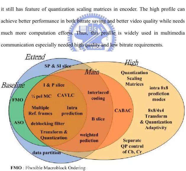
Fig 3 shows four profiles defined in H.264/AVC, which are baseline, main, extended and high profiles. Baseline profile includes basic coding tools and features, such as I-slice without intra 8x8 prediction modes, P-slice, quarter-sample accurate motion vector, deblocking filter, and CAVLC.

Main profile is used as the mainstream consumer profile for applications of broadcast system and storage devices. It contains most of the features in baseline profile and other advanced techniques, like adaptive frame/field coding, interlaced coding, weighted prediction, B-slice, and CABAC.

The extended profile, which includes all the features in baseline profile and main profile except CABAC, is intended as the streaming video profile and has relatively high compression capability with extra tricks for robustness to data losses and server stream switching.

Finally, the high profile is the most complex profile, Intra 8x8 prediction modes and transform and quantization of 8x8 block size are supported in this profile. Besides, it still has feature of quantization scaling matrices in encoder. The high profile can achieve better performance in both bitrate saving and better video quality while needs much more computation efforts. Thus, this profile is widely used in multimedia communication especially needed high quality and low bitrate requirements.

2.2.

Components of Intra Coding

2.2.1. Intra Prediction

Fig 4. Nine modes for intra 4x4 prediction

Fig 5. Nine modes for intra 8x8 prediction

Fig 6. Four modes for Intra 16x16 or 8x8 prediction

Spatial-domain prediction is the main feature of H.264/AVC intra coding. There are three kinds of intra prediction for luma components, nine 4x4 prediction modes, nine 8x8 prediction modes and four 16x16 prediction modes.

The 4x4 prediction modes use the neighboring thirteen reconstructed samples denoted from A to M in Fig 4 to predict the block pixels with eight different directions

and one average value. And all 8x8 prediction modes are very similar to the 4x4 prediction modes as shown in Fig 5. For 16x16 prediction modes, the values are predicted from the 32 adjacent boundary pixels of upper and left macroblocks. Similar procedures are also applied to the chroma components where four 8x8 prediction modes are used with 16 neighboring pixels.

2.2.2. Cost Generation and Mode Decision

The best mode decision for intra prediction in [10] can be either the time consuming rate distortion optimization (RDO) or just much simpler cost accumulation. RDO uses the weighted sum of actual encoded bitrate and the reconstructed samples to produce distortion. Though it can achieve better performance, it is computationally intensive.

An alternative way is using cost accumulation. Two generally used mode decision methods for cost generation are available in [10], sum of absolute difference (SAD) and sum of absolute transform difference (SATD). The best mode is finally decided by comparing the summarized cost value of sixteen 4x4 blocks in the 4x4 prediction, four 8x8 blocks in the 8x8 prediction and sixteen 4x4 blocks in the 16x16 prediction.

2.2.3. Transform

The transform can be divided into two parts, 4x4 or 8x8 integer transform and its fractional scalar multiplication factors that are further merged into the quantization stage. With this method, The DCT transform can avoid precision problem happened in previous standards. For a macroblock predicted by the intra luma 16x16 or intra chmora modes, the DC value of each transformed block is further processed by 4x4 DHT or 2x2 DHT. Besides, the inverse transform units have similar behavior with transform unit.

2.2.4.

Quantization and De-quantization

In the quantization stage, there are 52 values of quantization parameters (QPs) and corresponding quantization steps supplied in H.264/AVC standard. The steps are doubled for increase of every six numbers in QPs. The quantization scaling factors are to change transform of 4x4 or 8x8 block size becoming integer transform to avoid the computational complexity and precision problem.

Chapter 3

H.264/AVC High Profile HDTV Encoder

Video compression technique becomes more and more important while the development of mobile video device and HDTV is growing up. H.264, the latest video standard is well adopted in HDTV and other application since it provides high video quality and excellent coding efficiency. These coding tools provide high coding efficiency, however, also takes huge computational complexity and memory requirement, especially in intra encoding flow. Therefore, hardware accelerator for intra encoding flow of an H.264 encoder, especially which supports high profile, is necessary for real time encoding requirement.

3.1. Design Challenges of Intra Encoding in Our Encoder

Although the previous work [30] is an excellent design as the intra coding flow of baseline profile, we still have many challenges if we extend the previous design to the intra encoding of our high profile encoder. In the followings, we will show the proposed techniques to solve these problems.

z Cycle counts of every MB stage:

In previous work [30], we double the throughput of intra prediction phase. So we only need computing cycles less than 560 cycles. We extend this design to our high profile encoder that the cycle counts of all MB stages are 600 cycles. To support this design in high profile encoder we use the similar intra prediction algorithm in previous design [30] and scheduling the overall encoder function.

z Structure hazard of reconstruction phase

block size for intra prediction, reconstructing boundary pixels of 8x8 block size for intra prediction, and reconstructing data of the final mode as reference. This phase is independent in the third stage by three stage pipelined architecture, but intra mode decision in second stage needs reconstructed boundary pixels. To solve this problem, the process of reconstruction phase is through the second stage and the third stage. We can reuse the reconstruction phase in boundary pixel reconstruction of intra 4x4 and 8x8 prediction, and reconstruction data as inter reference by this method. The scheduling of the reconstruction phase is shown in Section 3.2.1.

z Reduce hardware cost:

In previous design [30], it uses the variable-pixel parallel architecture to reduce hardware cost and utilization of reconstruction phase. But the hardware cost for using this architecture to high profile is too high to afford. We use scheduling methods in Section 3.2.1 and in Chapter 4 to reduce such high hardware cost.

3.2.

Proposed Architecture

One challenge for high profile encoder is the special coding tools in main profile and high profile such as intra 8x8 prediction, 8x8 DCT, 8x8 quantization and de-quantization. If we extend current 4x4 prediction and DCT design to 8x8, the area will become four times than previous work. Therefore, hardware and memory share for these new coding tools and existing tools are necessary.

This section introduces the complete H.264 High Profile HDTV encoder. Fig 8 shows the block diagram of our proposed architecture. The encoder contains system control, bus arbiters, and six coding tools including: integer motion estimation (IME), fractional motion estimation (FME), intra prediction, reconstruction, deblocking filter engine, and entropy coding. Besides, internal SRAMs for reference data and residue data are also included in this design. The complete frame data and reconstructed result

are stored in external memory through bus arbiter and bus interface. The bus interface width is design for 128bits.

3.2.1.

Scheduling of Encoder

Fig 7. The scheduling of our encoder

Fig 7 shows the scheduling of these three stages expect entropy coding functions. There are three features in this scheduling. First, if all calculating MB orders are shown in Fig 7, we pre-load reference data for MB 3 in IME stage because of its high complexity. Second, FME and Intra can share residual SRAM and reference SRAM and load data from external memory in time by this special scheduling. Finally, the reconstruction process is through the second stage and the third stage.

During cycle 16 and 382 the reconstruction phase reconstructs data for computing intra prediction of MB 1 and filtering data of MB 0 and MB 1. Besides, after residual re-computation of a best mode is finished, the reconstruction is beginning to quantize them and reconstruct MB immediately in the second stage. This work continues to the third stage begins to finish the reconstruction of a MB and sends into the deblocking engine. By this method, we can quantize residuals needed by entropy coding in time to avoid waiting cycles in the third stage.

3.2.2. Function Units of Intra Encoding in our HP Encoder

[34][35] which use four stage pipeline architecture. The second stage is intra prediction and FME. The intra prediction works no matter current frame is I-frame, P-frame, or B-frame. The reconstruction is through the second stage and the third stage and the deblocking filer are placed in the third stage.

The partial data of left MB required by intra prediction is saved in local register for fast data access. Moreover, in this stage, after intra and FME prediction find their best mode and corresponding SATD cost, a final mode decision is also made in this stage. The final decision and its residue are saved to residue SRAM for further process. The reference data of final mode will be saved in the best ref SRAM for data reuse in reconstruction.

As for the reconstruction stage, its process is through the second stage and the third stage. During the second stage, it computes the reconstruction data for intra prediction of 4x4 and 8x8 block size. And after DCT transform in a best mode re-computation is finished, the reconstruction phase is beginning to quantize them and reconstruct MB immediately in the second stage. After the third stage begins, the reconstruction stage continues to finish the reconstruction of a MB and send it into the deblocking engine. When the reconstruction is finished, the deblocking engine filters the reconstructed MB and sends the final data to REC SRAM. Because the deblocking filter needs non-deblocking upper MB information, extra external memory is required to save the data of upper MB. The data in REC SRAM will be transferred to external memory by bus arbiter.

Fig 8. The block diagram of proposed H.264 high profile encoder

3.3.Conclusion

In this paper, we propose a high performance H.264 high profile encoder that can support 1080p resolution under 145MHz with smaller area. In the proposed design, we optimize the algorithm and architecture of intra encoding flow and pipelined schedule of the whole design to achieve a high throughput and low hardware cost design. Therefore, our design is much suitable for HDTV applications.

Chapter 4

Architecture Design of Intra Encoding Flow

In Chapter 3, an H.264/AVC high profile progressive encoder is proposed for high definition and all frame size video application. This design is proposed to support both encoding process for any frame size with high quality and low bitrate at the quite low clock rate. In this chapter, we describe the intra prediction, reconstruction and daglocking filter architecture in the encoder which is described in last chapter.

Since our previous work is codec, this encoding flow is also extended to codec design. In comparison with previous design, this work not only has the better quality with high profile encoding process but also supports up to the largest HD size 1080p. Furthermore, with the modified three-step fast prediction and enhanced SATD algorithm, this codec has the same computing cycles in every MB and increases acceptable hardware cost. Those characteristics make it more suitable for video application products especially high quality requirements such as mobile TV encoder, video conference, HDTV, and so on.

4.1. Design Techniques for Proposed Intra Prediction

Although this work is mainly based on the previous architecture [30], directly extended previous work to the high profile introduce various design problems, such as lengthy cycle counts, structure hazards, data hazards and large area cost. In the followings, we will show the proposed techniques to solve these problems.

z Independent intra 8x8 path for low cycle count:

the intra prediction phase needs 506 cycles to predict the best mode of intra luma 4x4, luma 16x16, and chroma 8x8 block sizes that the intra prediction mode of luma 8x8 block size is impossible to reuse the same hardware under our timing constraints.

The new path for predicting intra luma 8x8 modes is needed to be added in intra prediction phase with only necessary hardware.

z To modify the reconstruction phase to eight-pixel parallel architecture: If 8x8 transform in high profile is supported when we adopt four-pixel parallel architecture, the computing cycles for this transform is too many (32 cycles per transforming) and temporary register bits are too large when we still adopt 4-pixel parallel reconstruction architecture. So we need to modify the reconstruction circuits from 4-pixel parallel architecture to 8-pixell one.

z To schedule the SRAMs behavior between Intra and FME prediction:

The structure hazard occurs between Intra and FME prediction. For example, the residual coefficients need passing through quantization during computing cycles of the second stage. And reconstruction phase also need quantization circuits to reconstruct data. But we can’t use three quantization circuits which has large area in

our design. Furthermore, all SRAMs between 2nd stage and 3rd stage also have similar

structure hazards if we only use single port SARMs. The scheduling illustrated in previous chapter help us to avoid those hazards. How to use only one quantization circuits in our chip will be illustrated in Section 4.5.

z To increase the utilization of our design:

Although previous design uses the variable-pixel parallel architecture, its reconstruction phase still has only 11.4% utilization. To increase hardware utilization, we reuse the same reconstruction phase in boundary pixel reconstruction of intra 4x4 and 8x8 prediction, and reconstruction data as inter reference. With this method, the reconstruction phase in our chip can achieve 18.67% utilization. And the addition path in intra prediction can also have 56% utility by re-computation for intra 8x8 boundary values scheduling though this path is only for intra 8x8 prediction.

1. Reuse the reconstruction phase :

We remove the reconstruction circuits in intra prediction circuits and reuse

these functions from 3rd stage. We can save 69K hardware cost by this

consideration.

2. Avoid the structure hazard of quantization :

We don’t adopt ping-pong buffer architecture as show in previous work [30]. We place the quantization between the prediction residual buffer and entropy coefficients inputs buffer. Thus, we can quantize the prediction residual as entropy coefficients and reconstruct data as reference of other frames at the same time with only one quantization.

3. Reduce the temporary registers in additional path of intra prediction:

In intra 4x4 prediction modes, we uses the best residual buffer and prediction value buffer to reduce its boundary data reconstruction cycle time and complexity. But if we extend this method to intra 8x8 prediction modes, it needs ad least 2560 bits registers. This cost is so high that we adopt re-computation for intra 8x8 boundary values scheduling to save this cost.

4. Increase the utilization of reconstruction phase:

The method to increase the utilization of reconstruction phase is already illustrated. To support this method the functions in reconstruction can support not only 4x4 block size but also 8x8 block size.

5. Save the pipelined buffers between second stage and third stage:

One purpose in our chip is to save pipelined buffer. But it makes the structure hazards in second stage. We solve those hazards by overall scheduling illustrated in previous chapter and Section 4.5. With this scheduling the single port only prediction residual and reference SRAMs can be shared by intra and FME.

In previous work we use variable-pixel parallel architecture to save hardware. But it needs 1344 bits boundary registers at least to fit this architecture and make the computing cycles larger than 600 cycles. That’s one reason why we modify the reconstruction phase from 4-pixel parallel architecture to 8-pixel parallel one.

4.2. Description of Prior Art

4.2.1.

Survey of Fast Algorithm

For baseline profile encoding, intra prediction and SATD cost function for mode decision take almost 77% of computation in all functions [13]. This result is reasonable since there are so many modes to decision one best mode for a 4x4 block. Thus, the SATD function has to be applied to unnecessary prediction modes quite a lot. If we can reduce the computation of intra prediction and its related SATD transform, we can reduce much computation time and power. Thus, we select the modified three-step algorithm in [28] to decrease prediction modes efficiently with acceptable performance loss. As shown as Fig 9. Simulation results in [28] show that it can save about 23% of computation for the intra prediction and related transform with a bit-rate loss of 0.68%. Besides, this algorithm is suitable for the hardware implementation with little comparison circuit.

Fig 9. Decision flow of the modified three-step algorithm for intra prediction In determining the coding performance of H.264/AVC intra prediction quality, mode decision function is the most important part. To find a best matched prediction mode is to use RDO. Though RDO can provide the best performance, its high complexity hinders its usage in the hardware design. Thus, we adopt SATD method to predict the best mode. We combine the integer transform in [13] [14] and simplified multiplication factors called enhanced SATD (ESATD). The simplified multiplication factors are derived from quantization coefficients.

32 / 20 25 20 25 25 32 25 32 20 25 20 25 25 32 25 32 1 1 2 1 2 1 1 1 2 1 1 1 1 1 2 1 1 2 2 1 1 1 1 1 2 1 1 2 1 1 1 1 ) ( ⎥ ⎥ ⎥ ⎥ ⎦ ⎤ ⎢ ⎢ ⎢ ⎢ ⎣ ⎡ ⊗ ⎟ ⎟ ⎟ ⎟ ⎟ ⎠ ⎞ ⎜ ⎜ ⎜ ⎜ ⎜ ⎝ ⎛ ⎥ ⎥ ⎥ ⎥ ⎦ ⎤ ⎢ ⎢ ⎢ ⎢ ⎣ ⎡ − − − − − − ⎥ ⎥ ⎥ ⎥ ⎦ ⎤ ⎢ ⎢ ⎢ ⎢ ⎣ ⎡ ⎥ ⎥ ⎥ ⎥ ⎦ ⎤ ⎢ ⎢ ⎢ ⎢ ⎣ ⎡ − − − − − − = X X C ₍₁₎

And, we reduce prediction modes further. Macro blocks predicted in plane mode is only 4.2% in average and not larger than 5.7% except the sequence “Akiyo” which

contains much smoother texture. Thus, we remove plane mode prediction with 1% bit-rate loss, which can be easily compensated by ESATD.

4.2.2. Architecture Design in Previous Work

Boundary Reg for 4x4 Pixels Selection Di ff 8-point DCT DHT Pred. DC Reg

Cost Generator and Mode Decision Q IQ Boundary Reg for 16x16 8 to 4 Cur/Best Block Reg Source Input IDCT IDHT Ad d _{8 to 4 FIFO Reg} Rec. DC Reg Source Buffer 48x64 Single Port External Upper Line Buffer

Ping-pong Coefficient Buffer 104x48x2 Single Port CAVLC Encoder Intra Prediction Generator Upper Buffer Controller Bitstream Output Rec. Shifter Most Pb. Reg Source Reg Intra Prediction Generator Di ff

Prediction Phase Bitstream _Phase

8 pixels/cycle 4 pix/c 1 coef./cycle 4 pixels/cycle

Reconsturction Phase Quantization

Phase

Fig 10. Proposed architecture in previous work

The intra frame encoder design with the modified fast algorithm uses eight-pixel parallelism in the prediction phase but four-pixel parallelism in the reconstruction circuit. The eight-pixel parallel prediction phase which calculates two rows of one 4x4 block significantly improves the throughput and reduces the computing cycles for the computationally critical intra prediction generator by half. The total architecture includes a pair of boundary buffer, two intra prediction engines, an eight-input 4x4 transform, a cost generator with feedback signals for fast mode decision, and some registers. Since only blocks with best modes are allowed to pass through the quantization phase and reconstruction phase, these two phases adopt four-pixel

parallel architecture to save area. We use the current block and best block registers in the quantization phase and the FIFO registers to buffer the data. The bit stream phase, including CAVLC encoder, is similar to [11] with at least one coefficient per cycle.

4.3. Hardware Oriented Algorithm of Intra Prediction

Because the performance of the previous algorithm in [30] is not enough to encode the large frame size like 1080p which may work a little worse than original baseline profile in [10] as shown in Fig 16, we extend all fast intra prediction algorithms in previous work from baseline profile to high profile for this chip. For example, the 8x8 DCT transform and quantization are special functions which are not included in baseline profile. These functions are used in intra luma 8x8 modes prediction in high profile. Thus, we extend the ESATD function in previous work to intra luma 8x8 modes for computing its ESATD with 8x8 DCT transform (8x8 ESATD). For detail, because the multiplier of DC value is 0.25 in 4x4 DCT transform type and 0.125 in 8x8 DCT transform type, the shift parameter in 8x8 ESATD is one more than previous ESATD. Besides, the three step algorithm in [28] is also extended to intra luma 8x8 modes prediction and the plane mode is still removal. Table 1 shows all simulation results.

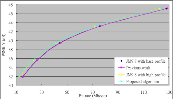
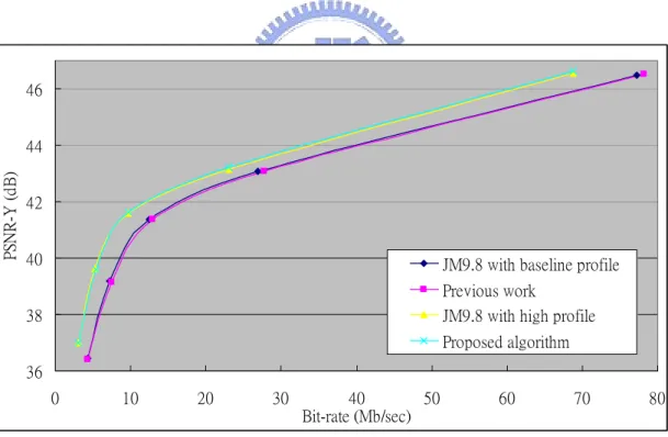
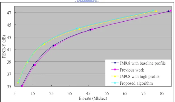
The Figures from Fig 11 to Fig 17 show the RD-curve diagrams of simulation results for all intra frame prediction by these four algorithms, original baseline profile algorithms, algorithm in [30], original high profile algorithm, and proposed one. We can find the obvious gap between the original high profile and baseline profile algorithm. It can be observed that the usage of the high profile algorithm can decrease 16.36% of bit-rate and increase 0.22 dB of PSNR in average. That’s the reason why we would like to develop this encoder.

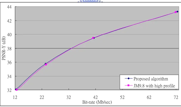
algorithm in [10]. The Figures from Fig 18 to Fig 24 show the RD-curve diagrams of their simulation results. In most case, the combined algorithm still makes the coding performance in all intra frame prediction much similar in high QP range and even better in low QP range.

Table 1 Comparison among original baseline and high profile in [10], previous algorithm, and proposed one for all intra frames with 1080p size

30 32 34 36 38 40 42 44 46 48 10 30 50 70 90 110 130 Bit-rate (Mb/sec) PS N R-Y (d B)

JM9.8 with base profile Previous work

JM9.8 with high profile Proposed algorithm

Fig 11. RD-curve of these four algorithm for sequence “blue_sky”

34 36 38 40 42 44 46 48 0 10 20 30 40 50 60 70 80 90 Bit-rate (Mb/sec) PS N R -Y ( d B )

JM9.8 with basline profile Previous work

JM9.8 with hig profile Proposed algorithm

32 34 36 38 40 42 44 46 48 5 25 45 65 85 105 125 Bit-rate (Mb/sec) PS N R -Y ( d B )

JM9.8 with baseline profile Previous work

JM9.8 with high profile Proposed algorithm

Fig 13. RD-curve of these four algorithm for sequence “riverbed”

36 38 40 42 44 46 0 10 20 30 40 50 60 70 80 Bit-rate (Mb/sec) PS N R -Y ( d B )

JM9.8 with baseline profile Previous work

JM9.8 with high profile Proposed algorithm

32 34 36 38 40 42 44 46 0 20 40 60 80 100 120 Bit-rate (Mb/sec) PS N R -Y ( d B )

JM9.8 with baseline profile Previous work

JM9.8 with high profile Proposed algorithm

Fig 15. RD-curve of these four algorithm for sequence “station2”

35 37 39 41 43 45 47 5 15 25 35 45 55 65 75 85 Bit-rate (Mb/sec) PS N R -Y ( d B )

JM9.8 with baseline profile Previous work

JM9.8 with high profile Proposed algorithm

32 34 36 38 40 42 44 46 5 25 45 65 85 105 Bit-rate (Mb/sec) PS N R -Y ( d B )

JM9.8 with baseline profile Previous work

JM9.8 with high profile Proposed algorithm

Fig 17. RD-curve of these four algorithm for sequence “tractor”

32 34 36 38 40 42 44 12 22 32 42 52 62 72 Bit-rate (Mb/sec) PS N R -Y ( d B ) Proposed algorithm JM9.8 with high profile

35 36 37 38 39 40 41 42 43 3 8 13 18 23 28 33 Bit-rate (Mb/sec) PS N R -Y ( d B ) Proposed algorithm JM9.8 with high profile

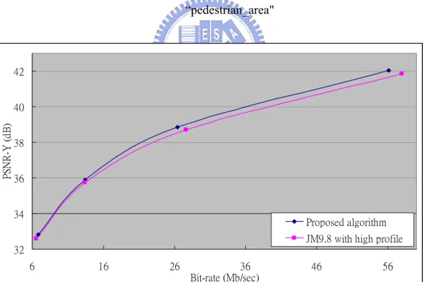
Fig 19. RD-curve of proposed algorithm and previous work for sequence “pedestrian_area" 32 34 36 38 40 42 6 16 26 36 46 56 Bit-rate (Mb/sec) PS N R -Y ( d B ) Proposed algorithm JM9.8 with high profile

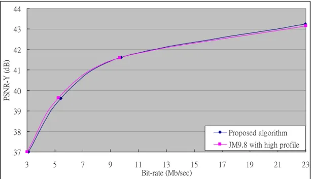
37 38 39 40 41 42 43 44 3 5 7 9 11 13 15 17 19 21 23 Bit-rate (Mb/sec) PS N R -Y ( d B ) Proposed algorithm JM9.8 with high profile

Fig 21. RD-curve of proposed algorithm and previous work for sequence “rush_hour"

33 34 35 36 37 38 39 40 41 42 43 0 10 20 30 40 50 Bit-rate (Mb/sec) PS N R -Y ( d B ) Proposed algorithm JM9.8 with high profile

35 36 37 38 39 40 41 42 43 44 45 5 10 15 20 25 30 35 40 Bit-rate (Mb/sec) P S N R-Y (d B) Proposed algorithm JM9.8 with high profile

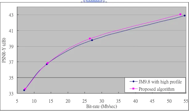
Fig 23. RD-curve of proposed algorithm and previous work for sequence “sunflower"

33 35 37 39 41 43 5 10 15 20 25 30 35 40 45 50 55 Bit-rate (Mb/sec) PS N R -Y ( d B )

JM9.8 with high profile Proposed algorithm

4.4. Architecture Design of Intra Prediction

4.4.1.

Overall Intra Prediction Circuit

This eight-pixel parallel prediction phase significantly improves the throughput and reduces the cycles for the computationally critical intra prediction path by half. But its throughput is still not enough to share the same hardware when we support intra luma 8x8 modes decision which increase 37.5% computation complexity. To solve this problem, we design the additional path to predict the best mode of intra luma 8x8 modes. To save hardware cost the three scheduling technique, parallel intra 8x8/4x4 computation, interlaced scheduling, and re-computation for intra 8x8 boundary values are used in this phase. We only add a pair of intra prediction engine, two 1-D eight-point eight-by-eight DCT transform, one more ESATD circuits, and a few small buffers. The total architecture includes two pair of boundary buffer, four intra prediction engines, an eight-input 4x4 transform, an eight-input 8x8 transform, two cost generator with feedback signals for fast mode decision, and some registers. Although the additional path also calculates 8 pixels at the same time, it’s different from previous work that these 8 pixels belong to one row of an 8x8 block.

In this section, we illustrate each component function in Fig 25. Boundary buffer stores the boundary of current MB or blocks in MB. And the prediction generators are duplicated and optimized with redundant datapath removal. The 4x4 DCT and cost function architecture are the same with previous work and the 8x8 DCT is also similar to 4x4 DCT. Finally, the Best buffer stores prediction residuals of one best mode and prediction value FIFO holds prediction reference value of the best mode to reconstruct boundary pixels. They are used only for modes of 4x4 transform type especially for luma 4x4 modes which needs a lot of cycles to reconstruct data.

To save too large hardware cost for intra luma 8x8 modes which behavior are the same as Best buffer and prediction value FIFO, we remove them by re-computation scheduling illustrated in previous section. By this method, we can save 2560 bits registers at least.

Fig 25. Intra prediction circuits in high profile progressive encoder

4.4.2.

Scheduling of Intra Prediction Phase

This scheduling of intra prediction generator as shown in Fig 26 is based on previous work. We used three scheduling technique in this scheduling, interlaced scheduling, parallel intra 8x8/4x4 computation, and re-computation for intra 8x8 boundary values.

z Interlaced scheduling :

The scheduling of luma 4x4 and l6x16 modes is interlaced the same as Fig 26. Because of changing reconstruction architecture to 8-pixel parallel, we re-schedule best luma mode, predict chroma mode, and re-compute chroma best mode in order

after luma mode decision.

z Parallel intra 8x8/4x4 computation :

Because we add the additional path for intra 8x8 mode decision, parallel intra 8x8/4x4 computation is used to computing intra prediction modes of 4x4 and 8x8 block transform type at the same time without happening structure hazards in reconstruction phase.

z Re-computation for intra 8x8 boundary values :

For additional path which is not including in previous work, we use re-computation for intra 8x8 boundary values to save hardware cost and increase its utilization. After the best mode decision of one 8x8 block, re-computation for intra 8x8 boundary values will re-compute its best mode two times, first re-computation is to re-compute boundary pixels as reference of its left and down block and final one is to produce the prediction reference value added with reconstruction residuals produced by previous re-computation. The paths of these two re-computation methods are shown in Fig 28 and Fig 29.

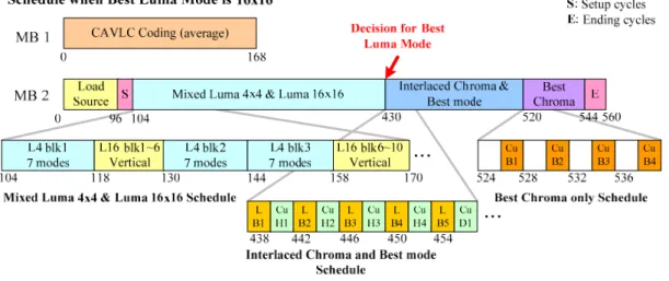
z Remove setup cycles in previous work [30] :

In Fig 27, the behavior of two blocks marked as Luma 8x8 Best mode and Luma 16x16 Best mode is to re-compute prediction residuals when the best luma mode is 16x16 or 8x8. Otherwise, the behavior of those two blocks is to do nothing. Besides, the purpose of setup cycles in Fig 26 is to compute DC value used in luma 16x16 dc mode. But we remove it and calculate the average value during computing ESATD value of luma 16x16 vertical and horizontal modes in our high profile chip to save calculating cycles.

Fig 26. Pipelined schedule for fast encoder when best luma mode is selected to 16x16 in previous work

Fig 28. Reconstruction path in first re-computation for intra 8x8 boundary values

4.4.3.

Intra Prediction Generator Unit

Fig 30 shows the eight-pixel parallel 4x4 intra prediction generator which is duplicated and optimized with redundant datapath removal and used for all modes expect intra luma 8x8 mode. Its behavior for some example modes is shown in Fig 31.

8x8 prediction generator is modified from 4x4 prediction generator to support some modes which need more than 6 inputs so that these modes can’t be implemented in original ones, like vertical right. We only add some multiplexers in 4x4 prediction generator to support more than 6 inputs. The behavior of 8x8 prediction generator is almost the same as 4x4 prediction generator, but it does not compute the prediction value of two row of a 4x4 block. It computes left and right 4 pixels in one row of an 8x8 block. We illustrate an example of one mode that 4x4 prediction generator doesn’t support. Its detailed architecture and that example are shown in Fig 32 and Fig 33.

Fig 30. Eight-pixel parallel intra prediction generator used for all modes expect intra luma 8x8 mode

Fig 33. Prediction value of left four intra prediction pixels in each 8x8 block row 7

4.4.4.

Transform Unit

Fig 34. Hardware architecture of transform unit

execute integer 4x4 DCT, 8x8 DCT, 4x4 DHT, and 2x2 DHT. In addition, two 4x4 block-size registers gather the DC coefficients for further DHT computation of DC blocks. The 2-D transform can also be separated into two 1-D transform with fast algorithm and butterfly architecture [16]. Since forward 4x4 DCT and DHT have the same butterfly structures and will not operate at the same time in the encoder, they can be merged together for area consideration. Similar architecture is applied to inverse transform. Fig 34 and Fig 36 shows the butterfly architecture of 1-D transform unit in 8x8 and 4x4 DCT transform.

Fig 36. Butterfly architecture of 1-D transform unit in 4x4 DCT transform

4.4.5. Cost Generation and Mode Decision Unit

Fig 37. Cost generation and mode decision unit

The cost function unit is implemented according to the enhanced SATD function illustrated in previous section. These current cost registers are used to temporarily

store the cost value for current mode. If the current mode belongs to the most probable modes, the non-zero initial cost value is given according to lambda value table instead of zero cost. If a smaller cost value is detected, the minimum cost value in 4x4 or 8x8 prediction modes is replaced by the new one and coefficients in the best block will be replaced by current ones. This comparing and replacing procedure will be continued recursively until the best mode with minimum cost is obtained. Similar operations are also applied to chroma components. Eventually, we will compare the minimum cost value between all luma modes again to determine which luma prediction type is used in this macroblock.

4.5. Memory Organization between 2

nd

and 3

rd

Stage

There are eight SRAM between 2nd stage and 3rd stage. Two store prediction

residuals of best mode selected from intra prediction or fractional motion estimation, four are used to store reference pixels, and the others hold coefficients after quantization. We share the prediction residual SRAM and reference data buffer between intra and inter prediction results by scheduling shown in previous chapter. The mean of numbers marked in Fig 39, Fig 41, and Fig 40 are block numbers which data is stored in SRAMs as show in reconstruction order of Fig 51 or row number of 8x8 blocks.

4.5.1. Connection between 2

nd

Stage and 3

rd

Stage

There are some differences in SRAM architecture between previous work and this design. We don’t continue adopting ping-pong buffer architecture so that we can reuse quantization circuits in reconstruction phase during computing coefficients for entropy coding. Besides, we can quantize them and reconstruct data as reference of inter frames at the same time with all single port SRAM. Fig 38 shows the connection

between the eight SRAM and 3rd stage. The prediction residual SRAMs store residuals from Intra or FME. Then it sends data into quantization when the reconstruction phase is beginning to reconstruct data. Finally the reference buffers hold the reference value of Intra or FME until the reconstructing phase needs them to do reconstruction adding.

Fig 38. Block diagram of reconstructing phase

4.5.2.

Prediction Residual SRAM

The memory organization of prediction residual buffer SRAM is shown as Fig 3939. It can store eight pixels per entry, as well as two rows in a 4x4 block or one row of an 8x8 block. Before selecting best luma mode, we store up residuals of any intra luma 4x4 mode the same as previous work [30]. If luma best mode is not intra 4x4, we replace SRAM data by the new one of that best mode.

Fig 39. Prediction residual SRAM between 2nd _{stage and 3}rd _stage

4.5.3. Reference Buffer

The reference buffer stores four pixels per entry. Fig 400 illustrates the block diagram of reference buffer that two 32-entries and 32-bits single port SRAM for luma components and two 16-entries and 32-bits ones for chroma reference. The behavior of these buffers is the same as residual buffers that we also store up the prediction value of intra luma 4x4 modes first and replace it if the luma best mode is not intra 4x4.

Fig 40. Reference buffer SRAM between 2nd _{stage and 3}rd _stage

4.5.4. Entropy Coding Data Inputs

We store the coefficients which are prediction residuals after quantization into coefficient buffers. These coefficient buffers has one 16 words x 224 bits x 1 bank memory for luma components and one 8 words x 192 bits x 1 bank memory for chroma one. It can store sixteen pixels per entry to reduce computing cycles of entropy coding that the entropy coding phase can load one 4x4 block data or two rows of an 8x8 block per cycle.

Fig 41. Coefficient buffer SRAM between 2nd _{stage and 3}rd _stage

4.6.

Components of Reconstruction Flow

4.6.1.

Overall Architecture of Reconstruction Phase

The reconstruction part also plays important role in our high profile encoder. It must reconstruct reference pixels of intra luma 4x4 block or intra luma 8x8 modes, and nearly every whole frame which will be a reference of other inter frames.

We modify the reconstruction circuit in previous work so that it can reconstruct data transformed by not only 4x4 block DCT transform type but also 8x8 block DCT transform type by 8 pixel parallel architecture. The main purpose of this change is to reduce the computing cycles of an 8x8 block IDCT transform by half, increase the utilization of reconstruction phase and remove the boundary registers between different pixel parallel phases.

4.6.2.

Quantization and De-quantization

Fig 43. Block algorithm of quantization circuits

In order to compute 8 pixels at the same time, we need to use a pair of quantize circuits modified from previous work like Fig 43. But we only need a quantization parameter table. For example, if we quantize data of one 4x4 block, we obvious the quantization parameters in every odd row and every even row are the same like what Table 2 shows. So that one quantization circuits only needs odd row parameters and the other one needs even row parameters. And this method is extended to quantize

8x8 block that one quantization circuits only needs left four parameters of one row and the other one needs right four parameters. Besides, we use similar architecture in de-quantization because of their similar function behavior.

Table 2 Quantization parameter table when QP equals twenty-eight: A for 4x4 block size, B for 8x8 block size

4.6.3. Inverse Transform Unit

Compare with other units of this chip, the reconstruction circuits has much lower utilization. To solve this problem, every design of this phase focus on multi-issues that we can not only reduce hardware cost but also raise the utilization. For example, the inverse transform unit can execute inverse 4x4 DCT, inverse 8x8 DCT, inverse 4x4 hadamard, and inverse 4x4 hadamard transform. This design is referenced in [31], so we also have structure hazards in [31] that when we just complete the computing of 4x4 DCT transform but the 8x8 DCT computing request comes immediately. We can avoid all structure hazards by the scheduling method of intra prediction phase and overall chip. Fig 44 is the block diagram of inverse transform unit.

Fig 44. Block diagram architecture of inverse transform unit

Fig 45 shows the architecture of 1-D transform unit that we only need to add several multiplexers from 8x8 DCT transform architecture to support those functions. Fig 46, Fig 47, and Fig 46 illustrate different datapath. First, we decide inputs site according to which function will be executed. Then, if the function is inverse hadamard transform, we avoid all shift paths in the figure. If the function is inverse 4x4 DCT transform, we execute down datapath of every multiplexer as shown in Fig 466. Otherwise, the up datapath of every multiplexer will be selected when executing

functions is 8x8 DCT transform. To avoid bubble cycles waiting for the DC value of special mode like intra 16x16 mode and intra chroma mode during reconstructing data, we compute inverse DHT transform after the DC value pass through DHT transform, quantization, and inverse quantization circuits immediately.

Fig 46. the 4x4 IDCT transform datapath in inverse transform unit

Fig 48. the inverse hadamard transform datapath in inverse transform unit

4.7.

Architecture Design of Deblocking Filter

4.7.1.

Overall Architecture of Deblocking Filter

Fig 4949 shows the deblocking filter architecture design in our chip. The deblocking filter phase continues using previous design in [32] developed by our group. Fig 500 shows the proposed full data reuse flow that maintain the same result as specified by the H.264/AVC standard. Starting from the left-top most block, we first do the horizontal filtering over its two vertical edges (edge 0 and edge 1). Then, since all data is available for horizontal edge 2, we can do the vertical filtering over this edge. This horizontal- vertical interleaved approach is repeated for each 4x4 block in raster scan order, as the edge number shown in Fig 50. This data flow is further improved to explore more data reusability.

Besides, there are two SRAM in this circuit. The SRAM named rec_SRAM in Fig 4949Fig 49 changes computing order as shown in Fig 511 and holds data passing through deblocking filter. Another SRAM holds data which does not complete filtering. The purpose that we hold data not complete filtering is to reduce data transferring cycles. We output data to external memory until we complete filtering data of one block row as shown in 1.1.1.

In 1.1.1, Un-filtered upper block means the upper reference of the down marcoblock. The hardware cost for storing up reference in chip is too large to sending it to external memory. For detail, the cost we store the up reference in 1080p frame size, we need to use 30720 bits SRAM at least. Filtering un-completed block means the nethermost four rows of one MB which are not filtered completed. So these four rows are transferred to external memory by the same reason. Otherwise, data sent to external memory is full filtered so that the external memory control can become easier.

Fig 50. Edge processing order for (A) luma edge, and (B) chroma edge

Fig 51. Computing order of blocks in different phase

4.7.2.Memory Organization and Behavior

The FSM of rec_SRAM in Fig 49 is shown in Fig 53. First, when the reconstruction phase is in reconstructing pixel state, the rec_SRAM stores those pixels to change computing order as shown in Fig 511. Then, against 1.1.1, we load the un-filtered pixels which are part of MB1 as inputs of deblocking filter circuits and store filtered pixels belong to MB0. Finally, the deblocking filter circuits become idle state after filtered data are outputted.

To reduce memory access cycles, every entry also stores data with special order. For example, the entry marked number two in Fig 54 stores 16 pixels which are all 16

pixels of block two by reconstructing order in Fig 51. But after filtering, it holds the third row of MB0 by top-down order. By this reordering, we can access every entry only with one cycle so that it can complete filtering in time under this restrictive computing cycle constraint.

Fig 52. Transferring data of deblocking filter

Fig 54. Rec_memory organization figure

The behavior of ext_SRAM is similar with rec_SRAM as shown in Fig 55 expect that all access of ext_SRAM is row order in every state. We hold pixels of previous calculated MB in ext_SRAM during idle state. After all pixels are reconstructed, it starts loading data into deblocking filter circuits and stores rows those complete vertical filtering but don’t complete horizontal ones. During the output request is asserted, the ext_SRAM sends data into external memory. Finally, the deblocking filter circuits become idle state after filtered data are outputted.

Fig 55. FSM of ext_SRAM

4.8.

Implement Result

4.8.1.

Gate-count of Proposed Intra Frame Encoding Flow

The intra frame encoding flow of the proposed high profile encoder with fast algorithm is designed by Verilog HDL and implemented using UMC 0.13µm technology. When synthesizing at 145MHz, the total gate-count is about 157K excluding the memory area. Table 3 Table 3 lists the final results of gate-count for each component. Comparing with previous work, the all increased hardware cost of this design is required for supporting high profile encoding especially for 8x8 transform ,quantization and de-quantization path. For example, although the gate-count in prediction stage has increased 26K, But the additional hardware, 8x8 prediction generators, 8x8 DCT transform, several boundary registers, and cost function calculator aren’t absent for supporting additional path under this acceptable clock rate. Otherwise, if we remove additional path and support high profile encoding, our working frequency will be at least 210 MHz. The total area may be larger than this design because of so critical timing constraint.

Table 3 List of gate count of intra encoding flow

Component [30] Proposed

architecture CMOS technology TSMC 0.13µm UMC 0.13µm

Synthesis clock rate 62.5MHz 145MHz

Intra prediction generator 3212 6646

DCT/DHT with DC registers 9193 19868

Cost generation and mode decision 9424 12923

Boundary prediction buffer 10074 16140

Schedule controller 1225 1176

Source buffer controller 1122 7248

Quantization and De-quantization 13427 31908

IDCT/IDHT with DC registers 6460 31903

Reconstruction 3328 6293

Deblocking filter N/A 22659

CAVLC 8179 N/A

CABAC N/A 6730

Total 65644 163464

4.8.2. Intra Frame Codec Design

Fig 56 shows the intra codec design with the same intra frame encoding data flow in this chapter. Table 4 shows the comparison among this design, [13], and previous work. Although the area of this codec is larger than previous work, it has higher PSNR by 0.31dB and lower bit-rate by 18.35% in average and 1080p frame size than previous one illustrated in section 4.2 and supports from the smallest QCIF to the