PII: !%005-1098(97)00053-8 Printed in Great Britain otm-1098/97 $17.ocl+ 0.00
Brief Paper
Basic Hardware Module for a Nonlinear Programming
Algorithm and Applications*
SHIN-YEU LINt
Key Words-Nonlinear programming; optimal control; nonlinear systems; nonlinear control; implementations; integrated circuits.
Abatraet-We present a VLSI-array-processor architecture for the implementation of a nonlinear programming algorithm that solves discrete-time optimal control problems for nonlinear systems with control constraints. We incorporate this hardware module with a two-phase parallel computing method and develop a VLSI-array-processor architecture to implement a receding horizon controller for constrained nonlinear systems. On the basis of current VLSI technologies, the estimated computing time to obtain the receding-horizon feedback-control solution meets the real- time processing-system needs. 0 1997 Elsevier Science Ltd. 1. Introduction
Discrete-time optimal control problems for nonlinear systems with control constraints are popular control problems. Numerous numerical techniques (Dyer and McReynolds, 1970) have been developed for solving this type of problem; however, computational efficiency is still a major issue that is frequently encountered in the solution methods. In this paper, we shall propose an algorithm that combines a projected Jacobi method and a Lagrange-dual Jacobi method to solve discrete-time optimization problems for nonlinear systems, which include discrete-time optimal control problems with control constraints. Our algorithm will achieve a complete decomposition effect, and the data and command flow within the algorithm are very simple and regular; these two factors suggest that our algorithm can be implemented by VLSI array processors to meet real-time processing- system needs. Thus the first contribution of this paper is the presentation of a VLSI-array-processor architecture for the implementation of our nonlinear programming algorithm. Implementing a computational algorithm by VLSI array processors to improve the computational efficiency has been a trend, especially in the area of signal processing; for example, Frantzeskakis and Liu (1994) deal with a least-squares problem with linear equality constraints. However, the nonlinear programming problem considered in this paper is more complicated because of the presence of nonlinearity and inequality constraints.
As well as applications to solving discrete-time optimal control problems for nonlinear systems, our hardward implementable algorithm has important applications to receding-horizon control. In recent years, there has been a * Received 15 June 1995; revised 3 June 19%; received in final form 31 January 1997. This paper was presented at the 3rd IFAC Symposium on Nonlinear Control System Design (NOLCOS), which was held in Tahoe City, CA during 25-28 June 1995. The Published Proceedings of this IFAC meeting may be ordered from: Elsevier Science Limited, The Boulevard, Langford Lane, Kidlington, Oxford OX5 lGB, U.K. This paper was recommended for publication in revised form by Associate Editor Matthew James under the direction of Editor Tamer Bapr. Corresponding author Professor Shin-Yeu Lin. Tel. +886 35 731839; Fax +886 35 715998; E-mail syhn@cc.nctu.edu.tw.
t Department of Control Engineering, National Chiao Tung University, Hsinchu, Taiwan.
1579
growing interest for the design of receding-horizon feedback controhers (Mayne and Michalska, 199Oa; Clarke and Scattolini, 1991; Mayne and Polak, 1993; Richalet, 1993; DeNicolao et al., 19%). For such controllers, stability is guaranteed for the zero-terminal-state strategy (Mosca and Zhane 1992: DeNicolao and Scattolini. 19941. The most distinguished characteristic of this controller compared with other control methodologies is its global stability for general nonlinear systems, as shown by Mayne and Michalska (199Oa. b. 1991): however, this is at the exoense of hieh ~ I. 1 computational complexity to obtain a control solution. Although model reduction is an attractive approach to reduce the computational complexity (Richalet, 1993) this approach may not apply to a general, especially a highly nonlinear, system. Thus, to cope with this computational difficulty, we have proposed a two-phase parallel computing method (Lin. 1993. 1994) to obtain the solution for receding-horizon feedback control. The phase 1 method uses a two-level (master- and slave-level) approach to solve a feasibility problem to obtain an admissible control and horizon pair. The control solution obtained in phase 1 is improved by phase 2, and the final solution is taken as the receding-horizon feedback control solution for the current sampling interval. The problems formulated in this two-phase method, except for the master-level problem in phase 1, are discrete-time optimization problems for nonlinear systems. Thus we can use our hardware-implementable algorithm as a basic algorithm module in the two-phase method, and this results in a simpler algorithm than that in Lin (1994) for solving a receding-horizon feedback control solution. Since the master problem in phase 1 can be solved by simple calculations, this suggests that the two-phase method can be implemented by VLSI array processes. Thus presenting a VLSI-array-processor architecture for a receding-horizon feedback controller is the second contribution of this paper. Since receding-horizon control is one of the most promising globally stabilizing control methodologies for highly nonlinear systems, the work described in this paper also represents an effort to realize a real-time controller for nonlinear systems.
2. Basic hardware module for a nonlinear programming algorithm
2.1. Statement of the the discrete-time optimization problem ofn nonlinear system. We consider discrete-time optimization problems for nonlinear systems of the form
min 2 yTM,y,,
Y ,G)
y,+,-Ky;+p(y,)=O, i=O ,... , N-l, (I) #(yN)=O. ,viC-yisY,, i=O ,..., N,
where the n X n matrix M, is positive-semidefinite, Y = (Yo,. . , Y,v), y; E R”, i = 0,. , N, are variables to be solved, K is an n x n constant matrix, p(yJ is a n-dimensional vector function of y,, JI( yN) = 0 represents the terminal constraints and I/I is a q-dimensional vector function, Y, and y, represent the upper and lower bound respectively of the variables y,. The discrete-time optimal control problem
for a nonlinear system with quadratic objective function and simple control constraints is a case of (1) under the conditions that
where I denotes the identity matrix and 0 denote the zero submatrix or zero vector function with appropriate dimensions; xi+, - xi -f(x,, ui) = 0 is the system dynamic equation. Note that the formulation in (1) can include the case of general control constraints; for the sake of simplicity, it is not discussed here, but the explanation can be found in Section 3.
2.2. The algorithm. To solve (l), we propose an algorithm that combines the projected Jacobi method with the Lagrange-dual Jacobi method. The projected Jacobi method uses the following iterations:
y,(f + 1) = y,(l) + y, dyf(l), i = 0, , N, (2) where y, is a step size and I is the iteration index. Here dy:(l) is the solution of the following quadratic subproblem:
m;‘” g0 ~YT &idy, + PfM)lTdyi,
E,(l) + dy,+, -‘Kdy, +p,#)dyi = 0, i=O,...,N-1 (3) +(y&)) + &,d,,U)dy, = 0
yi syy,(f) + dyi 5x, i = 0, . . , N,
where &(l) =~,+~(l) -KY,(~) +&y,(l)), p,(l) is the deriva- tive of the vector function p with respect to yi at y;(f), IL,,(f)
is the derivative of Cc, with respect to y,v at yN(f), dy,, i=O,..., N, are variables to be solved, and the diagonal matrix & is formed by setting the kth diagonal element m, as
mk= (
Mkk if Mkk > S, 6 otherwise,
where Mkk is the kth diagonal element of M, and 6 is a small positive real number.
It can b-e verified that if y,(fJ, i = 0, , N, is feasible then
dy:(f), i = 0,. . . , N, is a descent direction of (1); yi(f + l),
i=O ,..., N-l, is also feasible if OCy,=l. Thus the
projected Jacobi method is a descent iterative method, which converges and solves (1) if y, is small.
Since (3) is a quadratic programming problem with strictly convex objective function, by the strong duality theorem (Bazaraa and Shetty, 1979), we can solve the corresponding dual problem instead of solving (3) directly.
The dual problem of (3) is
m;x +(A), (4)
where the dual function
+
AT[Ei(l) +
dYi+l - KdYi + Py,(WY~ll +dyL
&&r., +
MvydOITdyN
+
G[$(xvW) +
clr,,(~)4d
(5)
is a function of the Lagrange multiplier A, E KY, i = 0, . . , N. We can use the following Lagrange-dual Jacobi method to solve (4):
Ai(t + 1) = A,(r) + y2 A&(t), i = 0,. . . , N, (6) where y2 is a step size, and AA(t) = (AA,(t), . . , AA&)) is obtained by solving the linear equations
diag [V:,@(A(t))] AA(f) + V,~$(h(r)) = 0. (7) Here @‘(A), the unconstrained dual function of 4, is defined
by relaxing the inequality constraints on primal variables of 4 as follows:
N-l
4“(A) = min c [My? fi&, +
[Mn(01’&
,=”
+ A?‘[&(0
+ dy,+
I - Kdyi +p,(WxlI
+ dy: &dy, +
bWvxwYOIT4,v
+ ~~[WdO~ + ~y,,iWYrv1~
(8)
where V$,,+“(A) is the Hessian matrix of @‘(A), diag[Vz,@(A)] is a diagonal matrix whose diagonal elements are taken from the diagonal elements of V:,@‘(A), and V,+(A) is the gradient of 4 with respect to A. Based on Luenberger (1984), V,4(A) and VZ,,@‘(A) can be computed by
i
E,(f) +&v,+,@(t)) - K& +p#)&(A(0),
V,,#(A(t)) = i=O,...,N-1, (9)
+(Y@)) + 3r,,(l)ciy~, i = N,
diag
[v~iA,9”W))l
=
{
-diagI[(-K + p,(l)lfil;‘[-K + p,(W + fi,F+‘,l,
i=O,...,N-1 (10)
-diag
[4Y,(f)fi,1&.Jf)Tl, i = N,where dyi(A(r)) E R”, i = 0,. , N, in (9) is the solution of the constrained minimization problem on the right-hand side of (5) with A = A(r). Since diag [V:,&‘(A(r))] is a diagonal matrix, we can compute AA(r) from (7) analytically by
AAi(r) = -{diag [V’,,+,&‘(A(r))]}-‘Vh,#A(r)), i = 0, , N, (11) It can easily be verified from (10) that diag [V:,9,<(A(r))]-’ is negative-definite. Thus AA,(r), i = 0,. . , N, obtained from (11) is an ascent direction of (4). Then the Lagrange-dual Jacobi method (6) will converge and solve (4) provided that yZ is small.
However, to calculate 0, 4(A(r)), we need the value of &(A@)), i = 0,. , N, whick can be found by the following two steps. First, we solve for the solution dyi, i = 0, . , N, of the unconstrained minimization problem on the right-hand side of (8), which can be obtained analytically by
&A(t))
1
fir’{-M,y,(f) - A,_, + [K -p,(l)lTA,}, i = 0, . , N - 1 = %‘[-M,YN(~) -AN-, - &,(~)‘4~1. i = N.
02)
Then, we project ri’y,, i = 0,. , N, to the constraint set y 5 y(f) + dy my, and the resulting projection dy,, i = 0,. , N, can be obtained analytically by
if y, ‘n(f) + &(A(r)) 5 Y,, &(A(r)) =
i
dyMr))
X -x(l) if yi(4 + &(A@)) >% 03) y, -y;(l) if Yj(l) + &(A@)) <y,,
i = 0,. . , N. It can easily be verified that dy,, i = 0,. , N obtained from (12) and (13) are indeed the solutions of the constrained minimization problem on the right-hand side of (5).
2.2.1. The complete decomposition property. In our algorithm, the projected Jacobi method performs only an update procedure in (2); all the major calculations lie in the iterations of the Lagrange-dual Jacobi method (6) for solving (4). Starting from -a given A(r), the Lagrange-dual Jacobi method solves &.CACt)j. ,,. ~ ,, i =O.. , N. from (12) and (13), then computes V,#(r)) and t;:,,,qF(A(r)), i LO:. , N: by (9) and (10) respectively. It then calculates AA?(r),
i = 0,. , N, from (ll), updates hi(r), i = 0,. , N, by (6) and proceed with the next iteration. This iterative process will continue until convergence occurs. From (6) and (9)-(13), we see that a complete decomposition effect has been achieved by our algorithm. This property results from (3) being separable.
2.2.2. The algorithm steps. Step 1. Step 2. Step 3. Step 4. Step 5. Step 6. Step 7.
Initially guess the values of y(0) and set I = 0. Compute K(l), p,(l), i = 0, . . . , N - 1, S(y,d)), and &,(O.
Initially guess the value of A(O), or set it as the previous value, and set t = 0.
Solve ay,(h(t)), i = 0, . . . , N, by (12) and (13). Compute V,.&+(t)) by (9), and diag [V&&“(A(f))] by(lO),i=d ,..., N.
Compute Ai(t + 1) = A&) - y*[diag (V:,,+‘)]-‘V,,
4(A(r)), i = 0, . . , N. Check whether IlAA(t)II, < E;
if yes, go to Step 7; otherwise, set t = t + 1 and return to Step 4.
Set dyt(f) = dyi(A(t)) and update yi(l + 1) = y,(l) + y,dyt(f), i = 0,. . . , N. Check whether IJdy*(l)(I, <
E; if yes, stop; otherwise, set I= I + 1 and return to Step 2.
2.3. The VLSI-array-processor architecture for implement-
ing the algorithm. Since both M, and diag [V~.,,#“(A)] are
diagonal matrices, A;’ and [diag(V$@‘(A~]-l can be computed analytically. Thus all the computations required in our algorithm steps are simple arithmetic operations, and are independent with each other on different time intervals owing to the complete decomposition property. This motivates us to implement the proposed algorithm using VLSI array processors by assigning a processing element (PE) to the computation required in a time interval of an algorithm step.
2.3.1. Modijkadon of the convergence criteria. Since our algorithm converges, the AA(r) in Step 6 and the dy*(l) in Step 7 will approach zero as the number of iterations t and I increase. Thus, instead of using a tolerance of accuracy, E, for convergence criteria in Steps 6 and 7, we may assign an arbitrary number of iterations I,,,,, for the Lagrange-dual Jacobi method and I,, for the projected Jacobi method, and modify the convergence criteria in Steps 6 and 7 as follows. Step 6(m). . . . If t 2 t,,,, go to Step 7; . . . .
Step 7(m). . . . If I 2 I,,,, stop; . . . .
2.3.2. The mapping of the algorithm steps lo the VLSI-array-processor architecture. Suppose we assign one
PE for performing the computation of an algorithm step in a time interval; all the PEs should be linked so that the data
and command flows in between PEs can make the PE arrays to perform the algorithm just as in a sequential computer. Thus the construction of the array-processor architecture should be based on the data and command flow in the algorithm steps. Examples of data flows are as follows: the data dyi(A(t)) and dy,+,(A(t)) computed in Step 4 are needed in the computation of V,d(A(t)) in Step 5; the data V,,4(A(t)) and V’,,*,&‘(A(t)) computed in Step 5 are needed in the computation of A,(t + 1) in Step 6(m). The command flow is more complicated; for example, in Step 6(m), if the Lagrange-dual Jacobi method converges, the data i?yi(A(t))
computed in Step 2 should be transferred to Step 7(m). This is a procedure of data flow followed by a command flow. In our algorithm, there are two types of commands: one is the initial-value request in Steps 1 and 3; another is the notification of convergence in Steps 6(m) and 7(m).
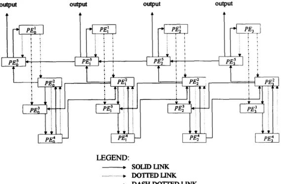
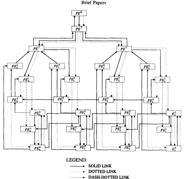
Figure 1 shows the VLSI-array-processor architecture for implementing our algorithm; for the sake of simplicity, but without loss of generality, we let N = 3 in Fig. 1. Each square block in Fig. 1 denotes a PE. The PEs lying in the same array will perform the same algorithm step. The directed solid links denote the data-transfer path. The directed dash-dotted links also denote the data-transfer path; however, they differ from the solid links in that receiving PEs will not use the transferred data for computation immediately. The directed dotted links in Fig. 1 denote the flow of commands of initial-value request or convergence notification. The arrows of these three types of links describe the data and command flows in the architecture.
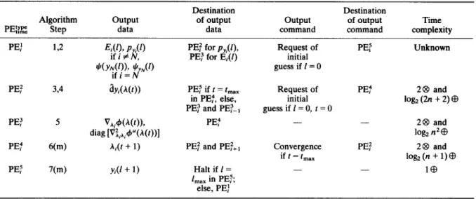
In the following, we shall explain the mapping of the algorithm steps to the architecture with the aid of Table 1. In the first column of the table, we indicate the type and the corresponding time interval of a PE by superscript and subscript respectively. The second column lists the corresponding algorithm step of each PE, which means that the computations in a time interval or a logical decision for convergence check carried out in an algorithm step will be performed in the corresponding PE. For example, PEZ will compute V,,4(A(t)) and diag [A:,,,,+‘(A(r))]. Although Steps 1 and 3 concerning the initial-value guesses do not require any computation, they will be taken care of by PE.! and PE? respectively. We shall explain how the initial values are provided when we introduce columns 5 and 6 of Table 1. Thus each algorithm step has a corresponding PE. The third and fourth columns show the output data and the corresponding destination of each PE, where the output data of a PE are its computed data. These two columns explain
output output
LEGEND:
-
soLlDLmK
_____...
. . .._... J’jomD JJN-K
_._._._._.+ D~H_~~D
LJJJK
Table I. The characteristics of PE
Destination Destination
Algorithm output of output output of output Time
PE:% Step data data command command complexity
PE: L2 F;$!$#) PE: for p,(f), Request of PE; Unknown
JI(Y$li)i &r)
PE: for E)(l) initial guess if I= 0 PE: PE: PE: PET 374 5 6(m) 7(m) dYM)) V*.+@(t)), diag
[~2,iA,4”O(~))l
A& + 1) Yi(l + 1) PET if t = t,, in PE?, else, PE) and PET-,PE:
PE: and PET+,
Halt if 1 = 1 max in PET; else, PE: Request of initial guess if I= 0, t = 0 - Convergence if t = t,,, PE: - PE: - 2@ and log2 (2n + 2) @ 28 and
log, n2cB
28 and log, (n + 1) CB l@the mapping of the data flow in the algorithm to the architecture, as described by the following examples. The data Et(l) (or $(y&) if i = N) computed in PE: is sent to PE), and the data p,(l) (or $,,,(I) if i = N) is sent to PEf. Since these data will not be used for computation immediately, the data Rows are indicated by dash-dotted links directed from PE: to PE: and PE: to PE: in Fig. 1. This corresponds to the data flow from Step 2 to Step 5. The output data ay, computed in PE: is sent to PEj) and PET-,, which is indicated by solid links directed from PE: to PE! and PET-, in Fig. 1. This corresponds to the data flow from Step 4 to Step 5. However, the data ay, will be sent to PE: if
t=t IWX; this is a situation of data flow followed by a command flow. The mapping of the data flows from Step 5 to Step 6, from Step 6 to Step 4 and from Step 7 to Step 2 can also be observed from the third and fourth columns of Table 1 and the directed solid links shown in Fig. 1. Columns 5 and 6 show the output commands and corresponding destinations of each PE. There are two types of commands: one is the request for initial guesses and another is the notification of convergence. As we have described earlier, Steps 1 and 3 concerning the initial guesses will be taken care of by PE: and PEf respectively. These steps are performed as follows. When I = 0, Step 1 needs an initial guess for y(f), and when I = 0 and f = 0, Step 3 needs an initial guess for A(f). Therefore, when I =O, PE: will output the command of initial-value request to PET, which will respond by sending a default value of y,(l) to PE). This command flow is described in columns 5 and 6 of the second row, and is indicated by the dotted link directed from PE,! to PET in Fig. 1. A similar situation occurs for PEf to request the initial value of A(r) from PE! when 1 = 0 and I = 0, as indicated in columns 5 and 6 of the third row in Table 1 and the dotted links directed from PE: to PE: in Fig. 1. For the convergence command, we see that if the iteration index f = t,,, is detected in PEY, it will output a command of convergence to PEf, as described in columns 5 and 6 of the fifth row. Then PET will respond by sending the data dyi(A(t)) to PET, as described in columns 3 and 4 of the third row in Table 1, which has not yet been explained. As shown in Fig. 1, this command flow is indicated by the dotted links directed from PEY to PEf, and the data flow followed by receiving the command is indicated by the solid links directed from PEf to PET. These command and data flows represent the mapping of the command and data flows from Step 6 to Step 7. However, when PET detects 1 = I,,,, it will halt the execution and output the solution, as described in columns 3 and 4 in the sixth row, which has not yet been explained.
2.4. Timing of the computations of the VLSI array processors. When using VLSI array processors to perform the algorithm, synchronization is necessary. In general, a global clock will cause severe time delay. Thus, to circumvent the drawback of global clock and maintain the synchroniza-
tion, the data-driven-computation PE (Kung, 1988) as- sociated with an asynchronous handshaking communication link (Kung, 1988) for data and command flows can be the solution. Therefore the computation in each PE will be activated after the completion of all the data transfers from the solid links; this will ensure that the computations in PEs lying in the same array are carried out asynchronously and simultaneously. Nevertheless, a self-timed clock is needed in each PE to control the synchronization of the operations in each individual PE.
2.5. Realization of PEs and time complexity. Basically, each PE consists of a self-timed clock, a control logic unit, two counters and a dedicated arithmetic unit. The typical structure of a PE is shown in Fig. 2. The self-timed clock is used to control the synchronization of the operations within the PE. The dedicated arithmetic unit may consist of multipliers, adders and various types of registers. Counter #l in Fig. 2 is used to count clock pulses in order to indicate the completion of the arithmetic operations. Counter #2 is available only in PE; and PET for each i, and detects whether t=t max or I= I,,, in the Lagrange-dual Jacobi method and the projected Jacobi method respectively. Note that once Counter #2 has reached the value of t,,, in PE: or I,,, in PET, it will be reset for next count of clock pulse. The functions of the control logic unit include the control of the sequence of arithmetic operations and the timing of the right communication link for sending out the data and
DAU
L!z
4 ICNl osc
LEGEND:
DAU - dedicated arithmetic unit CLU - control logic unit CNI - counter #l CN2 - counter #2 OSC - oscillator
reactions to the input command. For example, as shown in columns 3 and 4 of the third row of Table 1, and control logic circuitry in PE: should. determine which of the following solid links should be activated based on the value of the iteration index appearing in Counter #2: the solid link directed to PET or the solid links directed to PE: and PEf-,.
According to column 2 of Table 1 and the details of the algorithm steps, the structure of the dedicated arithmetic units of each PE can easily be realized by logical curcuitry and arithmetic units. For example, the formulas (12) and (13) for the computation of one component ~?y~, say ay{, in PET can be realized as in Fig. 3, in which part of the multiplexer is
used to perform the projection (13). From Fig. 3, we can derive the time complexity of the computations of PEY by taking the greatest p&sibie advantage of parallelism shown in column 7 of the third row of Table 1. where @ and @I denote the times required for performing a multiplication and an addition respectively. The time complexities for the commutations reauired for PE?. PE! and PE? can be obtained simiiarly to that’of PEf. However, the time complexity of PE,’ cannot be analyzed unless the function p(yi) is given.
2.6. Summary of the operations of VLSI array processors. We can summarize the operations of the VLSI array processors shown in Fig. 1 as follows. The computations starts from PE,‘, which commands PET to send the initial value of yi(l), and then computes E,(l) and p,(r). Ei(l) is sent to PET, while p,(l) is sent to PET. After recerving p,(l), PEj? commands PE? to send the initial value of A, and then calculates ay,, which is sent to PE: and PE:-,. After receiving ayi and ayi+,, PET will compute V,#(A(t)) and V:, @(h(t)), which are sent to PET. PE4 will then compute hilt’+ 1) and send to PE: and PET+,, provided that t < t,,,. The PE arrays formed by the PET array, PE: array and PE:
array will perform the Lagrange-dual Jacobi method until
t=t ,,_ is detected in PE:! When t = t,,,, the PEY array will command the PE: array to send the data ayi(A(t)) to the PET array. Then the PET array will update yi(l + 1) and continue the above process until I = I,,, is detected in PET and halt the execution.
3. Application to receding-horizon controller
3.1. The implementable receding-horizon controller. For a
nonlinear system with control constraints described by i = f(x(t), u(t)), u(t) E R, where f: R“ x RF’+ Wk is twice continuouslv differentiable and satisfies f(O. 0) = 0 and 52 is the set of admissible controls containing at&empty convex polytope, Mayne and Michalska (199Oa, b, 1991) proposed a globally stable implementable receding-horizon controller. Their control strategy employed a hybrid system i(t) = f(x(t), u(t)), when x(t) e W, i(t) = Ax(t) otherwise, where A =fx(O, 0) +fu(O, 0) is formed by applying a linear feedback
control u = Cx to the linearized system in a neighborhood W
with small enough radius and centered at origin, where C is
W-
the feedback gain matrix. Their algorithm first calculates an admissible control and horizon pair
[&I,
t,,,l E ZW(~Oh
(14) where the initial state x,) +! W is assumed, the set Z,(x) = {u E S, t, E (0, 2) 1 x”(t + $;x,t) E SW}, where S denotes the set of all piecewise-continuous functions, X” denotes the resulting state after applying the control u and6W denotes the boundary of W. The algorithm then sets h = 0, t,, = 0, uh = uo, tf,,, = t,,,, and performs the following
process repeatedly to yield the receding-horizon feedback control.
It applies the obtained control u,, for x 6 W and/or the linear feedback control Cx for x E W to the real system over
[t,,, th + At], where At E (0, z). Let x,,+~ be the resulting state
at t,,+,( = t,, + At); then, if x,,+, E W, the algorithm switches the control to u = Cx over (tic,, 2); otherwise, it calculates an improved control and horizon [u,,+, , tLh+,] in the sense that
[%+,, t,,+,l l Zw(%+,)*
(1% V(.G+I, (,,+I, $.,,+I) 5 V(xh+,r t,,+r, u,,, tf.h - At) where
,+,r V(x, I, u, t,) =
I I t(Ilx”(cx, t)ll&+ llu(r)ll2R)d~
in which R and Q are positive-definite matrices, l/y1151 denotes yTAy, and xL denotes the state trajectory in region
W with feedback control u = Cx.
The two-phase parallel computing method (Lin, 1994) aims to obtain a receding-horizon feedback control solution for every At time interval fi( r), t I 5 5 t + At, based on Mayne
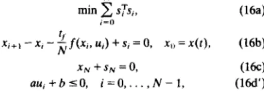
and Michalska’s algorithm. In the first phase, we discretize the system into N time intervals and use slack variables to formulate the following feasibility problem, which can also be called the phase 1 problem, to obtain an admissible control and horizon pair as required in (14):
(16a)
xi+,-X,-~f(Xi,Ui)+S,=O,
x0=x(t),Wb)
XN+SN=O,
ww
aui + b 5 0, i=O,...,N-I, (la’)
in which s denotes the vector of slack variables, and we explicitly express the non-empty convex polytope in R by the set of q-dimensional linear inequality constraints on
au + b s 0, where the matrix (I E Ryxp and the vector b E E?.
To apply the algorithm we proposed in Section 2, we need to
Y/(l)
M,’
Yi (4
4+,
P, Cl)Y
LEGEND: ( ’ )’ .- the jth component if
( ’ )is a vector
the jth row if
( . )is a matrix
reformulate the inequality constraints (16d’). First, we separate the simple inequality constraints ui 5 ui 5 r& from au; + b ~0, and then convert the rest of the inequality constraints to equality constraints a’u, + b + z, = 0 by adding positive variables zi, where a’ E RrxP, r or q. We can then rewrite (Xl’) as
a’u,+b+z,=O, ui=ui517,,
ZJZO, i=o ,...) /v-l. (164
If there is no simple inequality constraint for uir we may set i&=m and_ui=-m.
Suppose that the optimal objective value of the phase 1 problem (16a-d) under a proper horizon tf is zero; this tr and control solution is then the admissible horizon and control pair required in (14). Because tf is unspecified in (16a-d), we use a two-level (master- and slave-level) approach to solve the phase 1 problem (16a-d). The program in the master
,-.-I ,.c l l._ 6..._ I^..^ I --+I.^,4 :.. +,. A-a,...-:..- ^ . . ..l....l. :.. ‘C”Cl UI LUG Lvv”-LG”GL l‘lcilll”” I3 I” “CjL~ll‘llllS a Lf, WIUt,II 13
passed to the slave level, and the slave problem is (16a-d) with a fixed tf given by a master program. The master
program is simple; it increases rf by 8rf each iteration, where St, is a small positive real number. However, to increase the computational speed, we apply a gradient method for the first few iterations. Thus the master program (Lin, 1994) is as follows: f,(l + 1) = zr(l) + rd 2 fT(tf)f,(tf) dtfi=, if 2 ,=” ff(tf)9i(tf) > E, N tf(1 + 1) = Q(l) + St, if c s^,T(t,(l)s^,(t,(l)) < E and f 0, i=” stop otherwise, (17) where B(tf) denotes the solution of the slack variables in the slave problem under a given tr The slave problem is a case of the nonlinear programming problem considered in Section 2, which can be solved by the algorithm presented in Section 2. When the master program stops, the zero objective value of the phase 1 problem is achieved. This means that the .Amir.ihlr= rnnttnl smrl h&mm nair ir nhtaind I P+ In 7.1 ..-..I.YY.V.” _., . . . . “. . . . . . . . ..._“.. v”.’ .” .,“..._... --. ,.., ., , denote the admissible control and horizon pair obtained from phase 1 of the two-phase method; the phase 2 method will then improve [a, tr] in the sense of reducing the pcrformancc index V(x, t, u, tf), as required in (15). Thus, in phase 2, we shall solve the following phase 2 problem:
N-l
min c ($xTQx, + $u:Rui), i=o
if
xi+, -xi - ,f(Xi, Ui) = 0, xg = x(t), XN = 0,
(18)
a’ui + b + zi = 0, ui 5 ui 5 iii, zi 2 0, i = 0, . , N - i, which is a discretized version of (15).
We see that the phase 2 problem is also a case of the nonlinear programming problem considered in Section 2, and so can be solved by the algorithm presented in Section 2.
3.2. The VLSI-array-processor architecture and operations
for the implementable receding-horizon controller. The slave
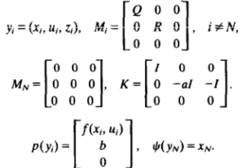
problem (16a-d) with a fixed C~ is a special case of (1) with appropriate dimensions. The phase 2 problem (18) is also a special case of (1) with
ro 0 0 02 Y, =
(Xi,
4, s,, Zi), M; = ; ; ; ;L
0 0 0 01
K= 0 -a’I 0 -I 0 0 0 0 0 0 0 0 f (Xi, 4) P(Yi) = “0 I 1 , #(Y,) = XN + SN,L
0J
where the 0s in M, and K and the 0s in pi(n) denote respectively the zero submatrix and the zero vector with appropriate dimensions. The phase 2 problem (18) is also a special case of (1) with
f(xi9 ui)
P(Yi)=
[
b1
7 ‘J’(YN)=XN. 0%..r l,,UJ L11.z l L, XIr cr a....“., . . . . ..nanrrrr ” LIuI-CzII(LJ-pl-c-l LLI~,,II~~,U,c, nml.:t~nt..-,X . ..~“.X..,~rl plrUCLX,tiU :” CZ’in 111 1 .a.
1 can readily be used to implement the solution methods for the solution methods for the slave problem and the phase 2 problem. Although the computing formulas for these two problems are the same, the data in these formulas are different. Therefore we need to use one bit to represent the mode for these two problems. We let 0 represent solving the slave problem and 1 represent solving the phase 2 problem. Thus this one-bit mode can be used to control a multiplexer to select the corresponding data, as shown in Fig. 4 for the calculation in PEs.
What remains for the architecture to implement in the two-phase parallel computing method is the master program in phase 1. As we have shown in (17), the master program is very simple. Thus we may use a processing element PEs to perform the formula given in (17). However, the data required in PE” should be provided from the solution of the slate problem from all time intervals. Let (f(+), a(+), O(t,), A@)) be the solution of the slave problem under a given tf; then we need PE” array processors to calculate the values of ST(t,)f&) and -fir(t,)(a/at,)f(2&), a(+)), and pyramid-like log, (N + 1) stage PE’ array processors. The PE’ array processors are two-input adders in the ~,nunrd rlirprtinn llr,=rl tn fnrm th.- c,,mc TN_. b’T(t.\B.lt.\ ..y....-- . . .._“.._.. ““II . . ..,.... . ..” -.. . . . . & ,=,,” ,\., r,\.J, and I% O(t,)(al+)f (ai( h(tf)), which equals (d/dtf) ZzoS:(f)Si(tf) (Lin, 1994). These are the data needed in PE to perform the gradient method when
Z~OST(tf)~&) < E. The PE’ array processors are registers in the downward direction used to propagate the value of t, computed in the master program to the slave
problem. Thus the overall VLSI array processors to implement the two-phase method are as shown in Fig. 5, in which the architectures of PE!, PEf, PET, PE; and PET arrays are almost the same as in Fig. 1, except for the addition of dotted links directed from PET to PE:, as expiained beiow. Because, when the siave probiem is soived for a given t,, the data A($) stored in PEY should be sent to PEP; these dotted links represent the fact that when PET detects convergence of the slave problem, it will command PEY to send data to PEF. Therefore there also exist solid links from PE4 to PEP in Fig. 5. Note that in phase 1, PEY will not halt the execution when detecting I = I,,,. This is different from Fig. 1.
3.3. The operations of the VLSI array processors for the
two-phase method. Initially, PEs will provide a value of t,(O)
and set the mode to be 0, and will pass down the value of
data for data for
Sh? Phase2
Fig. 4. The multiplexer controlled by the problem mode for selecting the corresponding data.
r-z-
LEGEND:
- SOLIDLINK
.. -t DOTTEDLINK
- - ---,t DASH-DOTTED LINK
Fig. 5. VLSI-array-processor architecture for the two-phase parallel computing method with N = 3.
r,(O) and mode 0 to the PE: array processors through the PE’ pyramid-like array processors, as shown by the solid links directed from PEs through the PE’ arrays to the PE: array in Fig. 5. Then the PE,!, PE?, PEj, PEf and PET arrays will perform the algorithm proposed in Section 2 to solve the slave problem under the value of r, given by PEs until convergence in PE: is detected, that is, when I = I,,,,.. The PET array processors will then output the values of 3i(tf) and (a/&r)f(f,, fi,) to the PEP array processors, and will command the PE4 array to send the data of Ai to PEP. The PE: will compute 3&~&) and hT(tr)(a/arr) f(.$(rr), ul,(r,)), and the PE’ arrays of processors will perform the sums CL3T(rf)3,(r,) and C;“=,, h^~(rr(alar,)f(~i(r,), G,(r ))
PE B
(=(d/d,,) CEo3T(rf), 3&), and input them to the processor to perform (17). This process will continue until PEs detects the convergence of the phase 1 problem, that is, ~f&-Ff(rf)3,(rf) = 0; then the value of the admissible horizon rf and the command of mode changing to 1 will be passed to the PE: array processors through the PE’ arrays. The mode-change command is indicated by dotted links directed from PE” through the PE’ arrays to the PE: array as shown in Fig. 5. The PE! array will then command the PEf, PE;‘, PE: and PE: arrays to change the mode to 1. For clarity, we do not show in Fig. 5 the dotted links for the rest of the mode-change command that occurs among the PE:, PE?, PET, PE;’ and PEj arrays. At this point, the solution of the phase 1 method, f,, P,, Z,, i = 0, . . . , N, is stored in the PET array. The PE!, PE:, PE?, PE4 and PE.5 arrays will then proceed to solve the phase 2 problem until I = I,, is detected in PE:, which will halt the execution and output the solution.
3.4. Overall-time complexity. From Section 3, we see that all the computations of the two-phase method he in the
Lagrange-dual Jacobi method; thus the total time complexity spent in the Lagrange-dual Jacobi method is the dominant term of the overall-time complexity. Let m, denote the actual numbers of iterations that the iterative two-level phase 1 problem takes to converge. Then the total number of iterations of the Lagrange-dual Jacobi method performed in phase 1 is m 1 I InaxfInaX~ Furthermore, the total number of iterations of the Lagrange-dual Jacobi method performed in phas ‘2 is 1 maxrmax. The time complexity of the array PEs should count as only that of one PE, since they are executed asynchronously and simultaneously. Let Tpa denote the time complexity of PEj, which is shown in column 7 of Table 1 in terms of numbers of @ and CB. Also, let TCL denote the time complexity of the asynchronous handshaking com- munication link, which is equal to 3 clock pulses according to the design in Kung (1988). Similarly, the time complexity of the array communication links should count as just one Tc_. Thus the total time complexity spent in the Lagrange-dual Jacobi method based on the above notation and the computing architecture shown in Fig. 5 is
(ml 5 max r max +I ma.~m&GE~ + TpEl + TPE4 + 37&). (19)
3.5. Simulations. According to the work of Yano et al.
(MO), G =3.8ns for a 16 X 16-bit multiplication, Tes 0.2ns for an addition, and the period of a clock pulse is approximately 40 ps. We may calculate that TPE2 = [7.6 + 0.2 tog, (2.n + 2)] ns, TpEl= (7.6 + 0.2 log, n’) ns, and TPE4 = [7.6 + 0.2 loga (n + l)] ns, according to column 7 of Table I, and r,- = 0.1 ns. Then (19) becomes
(mIr+I s max max maxtmax )
-1.5 L I
-1.5 -1 -0.5 0 0.5
(z”)Q Fig. 6. The final complete state trajectory for the example.
Example. The Rayleigh equation. x”=xa ) x,“=-1,
.@ = --xm + [1.4 - O.l4(xS)2] + 4u, n[ = -1, (21) where x” and xp are state variables and u is the scalar control. We intend to find a control solution that satisfies the instantaneous control constraints 1~15 0.7 and that drives the system from the initial state (-1, -1) at time t = 0 to (0,O) asymptotically. The following initial values are assumed in the phase 1 method: rr = 5 s, ui = 0, 05 i c N - 1, and xi” = xg - (i/N)xg, xf = xg - (i/N)xR, i = 0, 1, . . , N. The matrix
e=[:
iI
and R = 1 are used in phase 2. The linear feedback control II = --x” - 2x0 is employed in the region W = {x 1 blr I 0.5) to result in negative eigenvalues for the linearized closed-loop system at (0,O). The algorithmic parameters are arbitrarily assigned to be N = 30, E = 0.001, y, = y2 = y3 = 0.1, St, = 0.2 s, l,,, = 40, t,, = 40. Solving the example by our two-phase method-based implementable receding- horizont feedback control algorithm, we obtain h = 30 before reaching the region W, and the final complete state trajectory is shown in Fig. 6.
Estimated computation time for the two-phase method. In this example, n = 3 which is composed of two states and one control. For all h, including h = 0, we have m, = 1. The estimated computation time of the two-phase algorithm calculated from (19) is 0.08ms. . I This shows that the receding-horizon controller hardware meets the real-time processing system needs.
4. Conclusions
We have presented the architecture of a basic hardware module to implement a nonlinear programming algorithm that solves discrete-time optimal control problems for nonlinear systems with quadratic objective function and control constraints. We have applied this basic hardware module in the two-phase method, and it results in a simpler
algorithm than that in Lin (1994) for solving a receding- horizon feedback control solution. We have also presented the VLSI-array-processor architecture for this receding- horizon controller. The estimated computation time to obtain a receding-horizon feedback control solution is of the order of 0.1 ms, which meets the real-time processing requirement.
Acknowledgement-This research is supported by National Science Council, Taiwan under Grant NSC84-2213-E-009 132.
References
Bazaraa, M. and Shetty, C. (1979) Nonlinear Programming,
Wiley, New York.
Clarke; D. W. and Scattohni, R. (1991) Constrained receding horizon nredictive control. Proc. IEE. Pt D U&347-354.
DeNicolao: G. and Scattolini, R. (1994) Stability and output terminal constraints in predictive control. In Advances in Model-Based Predictive Control, ed. D. Clarke, pp. 105-121. Oxford University Press.
DeNicolao, G., Magni, L. and Scattolini, R. (1996) On the robustness of receding-horizon control with terminal constraints. IEEE Trans. Autom. Control AC4,451-453.
Dyer, P. and McReynolds, S. (1970) The Computation and Theory of Optimal Control. Academic Press, New York. Frantzeskakis, E. and Liu, K. (1994) A class of square root
and division free algorithms and architecture for QRD-based adaptive signal processing. IEEE Trans. Sig. Process. SP-42,2455-2469.
Kung, S. Y. (1988) VLSI Array Processors. Prentice-Hall, Englewood Cliffs, NJ.
Lin, S.-Y. (1993) A two-phase parallel computing algorithm for the solution of implementable receding horizon control for constrained nonlinear systems. In Proc. 32nd IEEE
Conf on Decision and Control., San Antonio, TX, pp. 1304-1309.
Lin, S.-Y. (1994) A hardware implementable receding horizon controller for constrained nonlinear systems.
IEEE Trans. Autom. Control AC-39,1893-1899.
Luenberger, D. (1984) Linear and Nonlinear Programming.
Addison-Wesley, Reading, MA.
Mayne, D. Q. and Michalska, H. (1990a) Receding horizon control of nonlinear systems. IEEE Trans. Autom. Control AC-35,814-824.
Mayne, D. Q. and Michalska, H. (1990b) An implementable receding horizon controller for stabilization of nonlinear systems: In Proc. 29th IEEE Conf on Decision and Control. Honolulu. HI. DD. 3396-3397.
Mayne, D. Q. and ‘Michaiska, H. (1991) Robust receding horizon control. In Proc. 30th IEEE Conf on Decision and Control, Brighton, UK, pp. 64-69.
Mayne, D. Q. and Polak, E. (1993) Optimization based design and control. In Proc. 12th IFAC World Congress,
Sydney, Australia, Vol. III, pp. 129-138.
Mosca. E. and Zhane. J. (1992) Stable redesinn of oredictive control. Automatic; 28,‘1229-1233. ” 1
Richalet, J. (1993) Industrial applications of model based predictive control. Automatica 29,1251-1274.
Yano, K., Yamanaka, T., Nishida, T., Saito, M., Shimohi- gashi, K. and Shimizu, A. (1990) A 3%ns CMOS 16 X 16-b multiplier using complementary pass-transition logic.