Approximate Analytical Description for
Fundamental-Mode Fields of Graded-Index Fibers:
Beyond the Gaussian Approximation
Qing Cao and Sien Chi, Fellow, OSA
Abstract—An approximate analytical description for funda-mental-mode fields of graded-index fibers is explicitly presented by use of the power-series expansion method, the maximum-value condition at the fiber axis, the decay properties of funda-mental-mode fields at large distance from the fiber axis, and the approximate modal parameters U obtained from the Gaussian approximation. This analytical description is much more accurate than the Gaussian approximation and at the same time keep the simplicity of the latter. As two special examples, we present the approximate analytical formulas for the fundamental-mode fields of a step profile fiber and a Gaussian profile fiber, and we find that they are both highly accurate in the single-mode range by comparing them with the corresponding exact solutions.
Index Terms—Fundamental mode, optical waveguide, power-se-ries expansion, single-mode fiber.
I. INTRODUCTION
T
HERE is much interest in the determination of the modal fields and the propagation constants of fundamental modes of graded-index fibers due to the great progress of single-mode fiber communication systems. However, exact analytical solu-tions are possible only for a limited class of index profiles, such as the step profile [1], [2], the clad parabolic profile [3], the power-law profiles [4], [5], and the infinite parabolic profile [6]. Even for these special profiles (except for the unphysical infi-nite parabolic profile [6]), the solutions [1]–[5] are still given in special functions or in the sum of many power series. In al-most all cases, one has to use either approximate or numerical methods. At present, it is possible to use numerical methods to obtain high accuracy, but one can not obtain much physical in-sight as with the analytical expressions presented by approx-imate methods. Among the approxapprox-imate methods, the simple Gaussian approximation [7] is good for the fundamental modes of graded-index fibers with large value (i.e., is near or larger than the cutoff frequency ). However, when the nor-malized frequency gets smaller, the Gaussian approximationManuscript received February 14, 2000; revised August 10, 2000. This work was supported by National Science Council of China under Contract NSC 88-2215-E-009-006. The work of Q. Cao was done while with the Institute of Electro-Optical Engineering, National Chiao Tung University and also with the Shanghai Institute of Optics and Fine Mechanics.
Q. Cao was with the Institute of Electro-Optical Engineering, National Chiao Tung University, Hsinchu, Taiwan 300, China, and also was with the Shanghai Institute of Optics and Fine Mechanics, Shanghai 201800, China. He is now with the Institut d’Optique, CNRS, B.P. 147, Orsay Cedex F-91403, France.
S. Chi is with the Institute of Electro-Optical Engineering, National Chiao Tung University, Hsinchu, Taiwan 300, China.
Publisher Item Identifier S 0733-8724(01)03557-5.
for the fundamental-mode fields becomes less accurate. In ad-dition, the Gaussian approximation can not correctly describe the fundamental-mode fields at large distance from the fiber axes. To improve the accuracy, many people have presented var-ious modified versions, such as the Gaussian-exponential [8], the Gaussian–Hankel [9], the generalized Gaussian [10], the ex-tended Gaussian [11], and the Laguerre–Gauss/Bessel expan-sion approximations [12]. These modified verexpan-sions are far more accurate than the simple Gaussian approximation. However, the optimizing processes of these modified variational methods are much more complicated than that of the Gaussian approxima-tion.
Unlike the high-order modes, the fundamental mode of a graded-index fiber has some special properties, such as the maximum-value point is always located at the fiber axis, the modal field is always larger than zero in the whole range of . As we show below, these special properties allow us to establish a simple power-series method to obtain the approximate fundamental-mode field when the modal param-eter is known. Fortunately, for those typical graded-index fibers, such as the power law profile fibers [4], [5], [7], [13] and the Gaussian profile fiber [13]–[16], the Gaussian approx-imation can still present highly accurate modal parameters in the single-mode range ([7, Fig. 14] and [13, Fig. 15-1], note that the normalized frequency of the practical single-mode fibers are usually in the range of ), though in this case the Gaussian approximation fails to provide the accurate fundamental-mode fields.
In this paper, we shall use the power-series expansion method, the maximum-value condition at the fiber axes, the positive-value property of the fundamental-mode fields, the decay property of the fundamental-mode fields at large distance from the fiber axes, and the modal parameters determined by the Gaussian approximation [7] to present a approximate analytical description for the fundamental-mode fields of graded-index fibers. In particular, as two special examples, we shall provide highly accurate closed-form formulas for the fundamental-mode fields of a step profile fiber and a Gaussian profile fiber.
II. PHYSICALCONSIDERATIONS ANDMATHEMATICAL
TREATMENTS
Let us consider a graded-index fiber whose radial index dis-tribution has the form
(1)
where
maximum index at the fiber axis; normalized radial coordinate; characteristic radius of the fiber core; radial coordinate;
total variation in the profile, ; profile function and satisfies the relations
and .
It is well known that the modal field and the propagation constant of the fundamental mode of a weakly guiding fiber satisfy the following eigen equation:[13]
(2) where , is the wavenumber in free space, is the wavelength in free space.
Substituting (1) into (2), and using the normalized radial co-ordinate to replace the radial coordinate , one can obtain
(3) where , is the normalized frequency,
, is the dimensionless modal parameter for fiber core.
Similarly to the evanescent field expression of the WKB method [17], we first express the modal field as the following form
(4) where is a normalization constant, is a real function of the variable . Apparently, this expression is consistent with the real physical phenomenon that the fundamental-mode field of a graded-index fiber, such as a power law profile fiber, is always larger than zero in the whole range of . Unlike the WKB method [17], we do not assume the triangular-function soultion because the fundamental-mode field has no node in the whole range of at all.
Substituting (4) into (3), one can obtain
(5) One may notice that [18] provided a similar treatment for the eigen equation of single-mode fibers. Especially, one can prove that (5) here is completely equivalently to (6) of [18] by taking the relation into account. This relation shows that our work is somewhat related to [18]. However, it is
be analytically expressed as , where is the modified Bessel function of the zeroth order and is given by . In terms of this relation, (4) and the assumption that the core-cladding interface is located at the point for convenience, one can obtain the boundary con-dition , where is the modified Bessel function of the first order. Obviously, this boundary condition is just [18, eq. (8b)]. In order to reduce the computation, [18] employed this boundary. However, we shall not use this boundary condition in the remainder of this paper. This is mainly due to the following two considerations. 1) We shall try to use some elementary function to approximately an-alytically describe the fundamental-mode field of single-mode fiber because of their simplicity. However, the modified Bessel functions appeared in the above-mentioned boundary condition are not elementary function. 2) Smooth profile functions such as the Gaussian profile function are very useful, even though, strictly speaking, those fibers with such smooth profile func-tions do not exist. However, for those smooth profile fibers, the boundary condition becomes invalid.
By use of (4) and the maximum-value condition at the point, one can prove that at the point. We then expand and the profile function (in this paper, we only consider those graded-index fibers whose profile function can be expanded as the power series for small ) as the power-series form
(6)
(7) in the region near the fiber axis, where we have used the proper-ties that and . One may notice that the power series of (6) and the power series of (7) are independent of each other, and therefore one can use two independent numbers to ex-press the powers of their highest-order terms that are taken into account, respectively. However, we use two related numbers and to express the powers of the highest-order terms of (6) and (7), respectively, because we hope the highest-order terms of has the same powers as that of in (5).
The high-order terms whose powers are higher than in the function and the high-order terms whose powers are higher than in the profile function have been ig-nored. Obviously, the expansion coefficients can be deter-mined by , where is the th-order derivative of at the point. The number of the terms of the power series for the function can be de-termined according to practical needs. Generally speaking, the
Substituting (6) and (7) into (5), and ignoring the high-order terms whose powers are higher than , one can obtain the following recurrence relations:
(8) (9)
(10) It is necessary to point out that these solutions are depen-dent on the modal parameter . In almost all cases, the exact values cannot be given in closed form. Fortunately, the simple Gaussian approximation can still provide highly accurate ex-pressions for the values in the single-mode range [7], [13] (as low as ). Therefore, we suggest to directly substitute the values that are obtained from the Gaussian approximation into (8)–(10) to approximately determine the concrete values of the parameters . It is worth mentioning that the power-series expansion method presented here is completely different from the previous power-series soultions for the fundamental modes of graded-index fibers [4], [5], [19]. The latter directly expand the fundamental-mode field as power-series and therefore has slow convergence property, but we now expand the function as power series and obtain a fast convergent solution. In fact, as we state above, in our expansion method, the first sev-eral terms are usually sufficient for the function .
Let us now investigate the asymptotic behavior of the funda-mental-mode field of a graded-index fiber at large . Similarly to the WKB approximation [17], from (5) one can deduce that and when , where is the modal parameter for the fiber cladding. There-fore, it is reasonable to use as the zero-order approximation at large , and then employ the perturbation method to obtain the first-order correction term . Simi-larly to the WKB method [17], in terms of (5) one can easily establish the following perturbation equation:
(11) for large , where the terms , and have been ignored. From (11), one can obtain
(12) where we have ignored the term because it is usually far smaller than the two terms of the right-hand side of
(12) for large . For example, for a power law profile fiber, the term is exactly equal to zero in the range of .
We then use the following method to joint the two kinds of solutions that are given by (6) and (12), respectively. When
, the function is given by (6), and when , the function is given by (12), where the joint point is determined by the equation
(13) One can easily prove that (13) can ensure that the funda-mental-mode field and its first-order derivative are both continuous at the joint point . One may want to know whether or not the joint point used here is related to the so called turning point used in the WKB method [17]. We point out that they are completely different. The former is defined by (13), but the latter is determined by the relation [17]. As we point out before, the fundamental-mode field and its first-order derivative are both continuous at the joint point ; but according to the WKB method, the modal field is divergent at the turning point . In addition, we also want to emphasize the well-known result that the WKB method is invalid for the fundamental-mode field. Therefore, we do not discuss the turning point problem in this paper. In practical applications, (13) can be easily solved by numerical approach.
After obtaining the coefficients and the joint point , one can analytically express the fundamental-mode field as the closed form (14) shown at the bottom of the page.
One can obtain a more accurate value than that of the Gaussian approximation if one substitute the solution of (14) into the expression
(15)
which can be derived from (3) and (4), because the solution given by (14) is more accurate than the corresponding Gaussian approximation solution. In order to understand this statement better, we shall present two concrete numerical results in Sec-tions III-A and -B.
,
It is interesting to explain why the fundamental-mode field of a graded-index fiber has an approximate Gaussian distribu-tion when the normalized frequency becomes large. Our the-oretical treatments imply a good explanation. If one let
, then one can obtain the zero-order approximation
, which is a Gaussian distribution. One may notice the interesting result that the width of this Gaussian dis-tribution is only (directly) related to the modal parameter . Usually, when the normalized frequency becomes large, the terms ( ) become negligible with the first term before the first term
has become rather large. As a consequence, in this case, the zero-order approximation is a good one in the region where the modal field is remarkably different from zero. This is why the fundamental-mode field of a graded-index fiber shows a nearly Gaussian distribution when is large.
III. EXAMPLES
To understand the above analytical description better, let us now present two special examples. One is the funda-mental-mode field of a step profile fiber, the other is the fundamental-mode field of a Gaussian profile fiber. These two kinds of graded-index fibers are both typical. Therefore, the investigation on their fundamantal-mode fields has practical meanings.
A. The Step Profile Fiber
For a step profile fiber whose profile function is given by for and for , the expan-sion coefficients are determined to be for all orders. Substituting these relations into (8)–(10) and letting , one can obtain , ,
, , and
, where the modal parameter is approximately given by according to the Gaussian approxima-tion [13], [14]. Substituting the coefficients and the relations and into (13), one can determine the joint point . The change of with the variable is shown in Fig. 1. From Fig. 1 one can see that is nearly invariant in the range of . To more conve-niently use the approximate analytical formulas of (14), we now use the approximate expression
(16) to fit the function in the single-mode range. From (16) one can find that is a approximate parabolic function in the range of and is approximately equal to 1.0 in the
Fig. 1. Functional relation between the normalized radial coordinateR (V ) of the joint point and the normalized frequencyV : The step profile fiber.
(a)
(b)
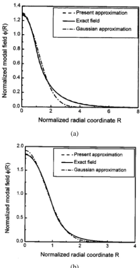
Fig. 2. Comparison among our approximate formula, the Gaussian approximation and the exact solution: The step profile fiber: (a)V = 1:5 and (b)V = 2:5.
Fig. 3. Functional relation between the normalized radial coordinateR (V ) of the joint point and the normalized frequencyV : The Gaussian profile fiber.
(17), shown at the bottom of the next page, where is given by (16), , , , , , and are given in the first paragraph of this subsection. The exact modal field, the approximate ana-lytical formula presented here and the Gaussian approximation for and are shown in Fig. 2, where the field distributions have been normal-ized according to , is the normalized con-stant. From Fig. 2 one can see that our expression is far more ac-curate than the Gaussian approximation and still valid for small values. In order to test the accuracy of (15), we also evaluate the value corresponding to by employing (15). In this case, the exact value is ; the value determined by the Gaussian approximation is ; and the value determined by (15) is . From thses results, one can find that, just as we predict in Section II, the value determined by (15) is more accurate than that determined by the Gaussian approximation.
B. The Gaussian Profile Fiber
For a Gaussian profile fiber whose profile function has the form , the expansion coefficients are determined to be for all even m and
for all odd . Substituting and the relation , which is obtained from the Gaussian approximation [13], [14], into (8)–(10) and letting , one can obtain
, ,
, ,
(a)
(b)
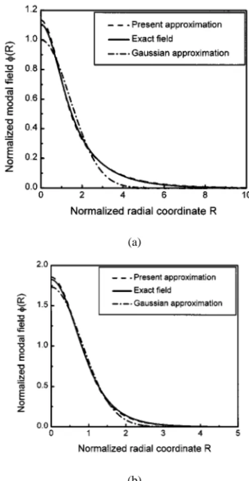
Fig. 4. Comparison among our approximate formula, the Gaussian approximation and the exact solution: The Gaussian profile fiber: (a)V = 1:5 and (b)V = 2:5.
and . Substituting these coefficients and the relations and
into (13), one can determine the joint point . The change of with the variable is shown in Fig. 3. The functional relation can be well fitted by the approximate expression
(18) The error of (18) with the exact value is less 0.25% in the range of and less than 0.45% in the range of . From (18) one can find that is a approximate parabolic function in the range of and is a approximate linear function in the range of . From Fig. 3 one can further find that the total change of in the range of
(19)
is very small and the central point is about . Similarly to the step profile fiber, the fundamental-mode field of a Gaussian profile fiber can be expressed as the closed form (19), shown at the top of the page, where is given by (18), and , , , , , and are given in the first paragraph of this subsection.
The exact modal field (we use the numerical method pre-sented by [15] to obtain the exact numerical solutions), the ap-proximate analytical formula presented here and the Gaussian approximation for and are shown in Fig. 4, where the field distributions have been normalized according to , is the nor-malized constant. Again, the high accuracies of our approxi-mate analytical description are observed. We also evaluate the value corresponding to by employing (15). In this case, the exact value is ; the value determined by the Gaussian approximation is ; and the value determined by (15) is . Again, we find that the value determined by (15) is more accurate than that determined by the Gaussian approximation.
IV. CONCLUSION
We have presented an approximate analytical descrip-tion for fundamental-mode fields of graded-index fibers by use of the power-series expansion method, the max-imum-value condition of the fundamantal-mode field at the point, and the decay law at large . This new analytical description is much more accurate than the Gaussian approximation and at the same time keep the simplicity of the latter. As two special examples, we have presented the analytical approximate formulas for the fundamental-mode fields of a step profile fiber and a Gaussian profile fiber, and found that they are both highly accurate in the single-mode range by comparing them with the exact solutions. The results obtained in this paper can be used to conveniently evaluate the relevant parameters of a single-mode graded-index fiber.
ACKNOWLEDGMENT
The authors are indebted to the reviewers for their comments and proposals for improving the paper.
[3] R. Yamada, T. Meiri, and N. Okamoto, “Guided waves along an op-tical fiber with parabolic index profile,” J. Opt. Soc. Amer., vol. 67, pp. 96–103, 1977.
[4] W. A. Gambling, D. N. Payne, and N. Matsumura, “Cut-off frequency in radially inhomogeneous single-mode fiber,” Electron. Lett., vol. 13, pp. 139–140, 1977.
[5] J. D. Love, “Power series solutions of the scalar wave equation for cladded, power-law profiles of arbitrary exponent,” Opt. Quantum
Electron., vol. 11, pp. 464–466, 1979.
[6] D. Marcuse, Light Transmission Optics, 2nd ed. Malabar, FL: Krieger, 1989, ch. 7.
[7] , “Gaussian approximation of the fundamental modes of graded-index fibers,” J. Opt. Soc. Amer., vol. 68, pp. 103–109, 1978. [8] A. Sharma and A. K. Ghatak, “A variational analysis of single mode
graded-index fibers,” Opt. Commun., vol. 36, pp. 22–24, 1981. [9] A. Sharma, S. I. Hosain, and A. K. Ghatak, “The fundamental mode
of graded-index fibers: Simple and accurate variational methods,” Opt.
Quantum Electron., vol. 14, pp. 7–15, 1982.
[10] A. Ankiewicz and G. D. Peng, “Generalized gaussian approximation for single-mode fibers,” J. Lightwave Technol., vol. 10, pp. 22–27, 1992. [11] S. C. Chao, W. H. Tsai, and M. S. Wu, “Extended gaussian
approxima-tion for single-mode graded-index fibers,” J. Lightwave Technol., vol. 12, pp. 392–395, 1994.
[12] G. De Angelis, G. Panariello, and A. Scaglione, “A variational method to approximate the field of weakly guiding optical fibers by Laguerre-Gauss/Bessel expansion,” J. Lightwave Technol., vol. 17, pp. 2665–2674, 1999.
[13] A. W. Snyder and J. D. Love, Optical Waveguide Theory. New York: Chapman & Hall, 1983, ch. 15.
[14] A. W. Snyder, “Understanding monomode optical fibers,” Proc. IEEE, vol. 69, pp. 6–13, 1981.
[15] R. S. Anderssen, F. R. de Hoog, and J. D. Love, “A numerical technique for solving the scalar wave equation for gaussian and smoothed-out pro-files,” Opt. Quantum Electron., vol. 13, pp. 217–224, 1981.
[16] Y. Ohtera, O. Hanaizumi, and S. Kawakami, “Numerical analysis of eigenmodes and splice losses of thermally diffused expanded core fibers,” J. Lightwave Technol., vol. 17, pp. 2675–2682, 1999. [17] S. Schiff, Quantum Mechanics, 3rd ed. New York: McGraw-Hill,
1968, ch. 8.
[18] E. K. Sharma, A. Sharma, and I. C. Goyal, “Propagation characteristics of single mode optical fibers with arbitrary index profiles: A simple nu-merical approach,” IEEE Trans. Microwave Theory Tech., vol. MTT-30, pp. 1472–1477, 1982.
[19] W. A. Gambling and H. Matsumura, “Propagation in radially-inhomo-geneous single-mode fiber,” Opt. Quantum Electron., vol. 10, pp. 31–40, 1978.