Building 22, 195-3 Chung Hsing Road Section 4
Chutung, Hsin Chu 310 Taiwan
Mao-Hong Lu,MEMBER SPIE National Chiao Tung University Institute of Electro-Optical Engineering 1001 Ta Hsueh Road
Hsin Chu 30050 Taiwan
E-mail: mhlu@jenny.nctu.edu.tw
of the focused beam as a function of input beam waist to lens spacing, lens-to-target plane spacing, input beam Rayleigh range, and focal length of lens. From this expression, we get the depth of focus (DOF) of flying optics with a fixed flying range, which is used as a merit function to determine the optimal solutions for system parameters. The results are very useful in the design and analysis of flying optics in laser material processing. Finally, a practical example describing the optimization of the output coupler for CO2laser resonator is given. © 1998 Society of Photo-Optical Instrumentation Engineers. [S0091-3286(98)02505-7]
Subject terms: Gaussian beam; beam focusing; flying optics; depth of focus; la-ser material processing.
Paper 37047 received Apr. 30, 1997; revised manuscript received Oct. 23, 1997; accepted for publication Oct. 29, 1997.
1 Introduction
Due to the beam feature, the behavior of a focused Gauss-ian beam can not be precisely approached to the practical level by geometrical optics. Based on a simplified model in which nontruncating, thin-lens, aberration-free, and on-axis optical systems are assumed and the thermal-lensing effect is neglected, the expressions of output beam parameters are derived with ray transfer matrix and mode matching in the review paper of Kogelnik and Li.1From diffraction theory, Dickson2derived a somewhat more general expression in-cluding aperture truncation effect. With the safe truncation in which the radius of the physical aperture is twice larger than the 1/e2 radius of Gaussian beam at the aperture, this
more general expression reduces to the Kogelnik and Li’s expression. To be analogous to geometrical optics, Self3 simplified this derivation and got concise expressions de-scribing the variations of beam waist radius, Rayleigh range, and beam waist to lens spacing for a focused Gauss-ian beam as a function of those of input beam and focal length of lens. Luxon et al.4verified Self’s equations to be valid for all higher order modes and useful in practice.
In laser material processing, the power density ~irradi-ance! of working beam has a tolerance range for a particu-lar application. If the range is exceeded, it results in poor quality or even cessation of the process. As a fixed laser power is applied during processing, this tolerance makes a constraint on the acceptable variation in the value of work-ing beam radius. The depth of focus~DOF! is defined as a distance from the focusing point over which the working beam radius varies within the required region. In flying optics, beam guiding over long distance during processing changes the input beam waist to lens spacing and results in the variations of beam waist radius, Rayleigh range, and beam waist to lens spacing of working beam. Much work has been done to reduce these variations. Luxon5optimized the surface curvature of output coupler in Spectra-Physics
825 configuration CO2 laser resonator. Zoske and Giesen6
optimized the interspacing of beam expander. Haferkamp et al.7used adaptive optics~deformable mirror! to compen-sate the variation of input beam waist to lens spacing.
In this paper, a general expression is derived to describe the variation of 1/e2 radius of focused Gaussian beam as a function of input beam waist to lens spacing, lens-to-target plane spacing, input beam Rayleigh range, and focal length of lens. From this expression, we get the DOF of flying optics with a fixed flying range, which is used as a merit function to find out the optimal solutions for system param-eters. The results are very useful for the design and analysis of flying optics in laser material processing.
Finally, we provide an analysis example of the optimum design of output coupler in laser-gantry-robot systems to show how to use our derived equations to find the optimal parameters and the DOF value.
2 The 1/e2 Radius Equation of the Focused Gaussian Beam
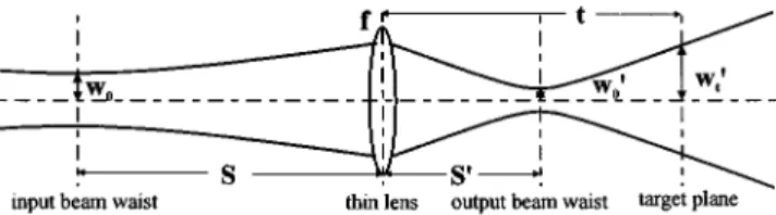
Based on the mentioned simplified model of Gaussian beam focusing, the geometry and parameters of focused beam, as shown in Fig. 1, can be well described by Self’s equations. We summarize his equations as
H
w08
5mw0 Zr8
5m2Zr s8
5 f 1m2~s2 f ! , ~1a! whereH
m5F
f 2 ~s2 f !21Zr2G
1/2 w05S
lZr pD
1/2 . ~1b!With Self’s convention w0, Zr, s, w0
8
, Zr8
, and s8
are waist radii, Rayleigh ranges, and beam waists to lens spac-ings of input and output beams, respectively. The s is posi-tive if the input beam waist locates in front of lens, but the s8
is positive if the output beam waist locates behind lens. Both m and f are magnification and focal length of lens, respectively.The equation for the 1/e2 radius of a focused Gaussian beam at the target plane after lens ~see Fig. 1! can be de-rived with Eqs.~1a! and ~1b! and expressed as
w
8
~s,t;Zr, f !5w08
F
11S
t2s8
Zr8
D
2G
1/2 5S
lZrp f2H
~t2 f ! 2 1F
~t2 f !~s2 f !2 f 2 ZrG
2JD
1/2 , ~2! and w8
~t[ f ;s,Zr!5S
l f 2 pZrD
1/2 . ~3!Equation ~2! describes the output beam radius w
8
, which varies as a function of the parameters s, t, Zr, and f . From Eq.~3! we can see that the output beam radius w8
at back focal plane is independent of the s value. This feature was also noted by Dickson.2Now, we can express the output beam radius in a nor-malized form as
wnor
8
~x,y!5w8
~s,t;Zr, f ! w8
~t[ f ;s,Zr!5@y21~xy21!2#1/2 ~4a!
5
F
~11x2!S
y2 x 11x2D
2 111x1 2G
1/2 , ~4b! whereH
x5~s2 f !/Zr y5~t2 f !Zr/~ f2!. ~4c!From Eq. ~4b!, we can see that the output beam waist lo-cates at the position y5x/(11x2) and the normalized
ra-dius at waist reaches the minimum value as 1/(11x2)1/2.
3 DOF Features in Nonflying Optics
With a fixed input beam-waist-to-lens spacing during pro-cessing, s remains constant and the system is called non-flying optics here. From Eq. ~4b!, it can be seen that the focusing point can be clearly chosen as the position of out-put beam waist for the minimum value of focused beam radius. As with Eq.~1a!, the focusing point is usually dif-ferent from the focal point of lens except that s5 f . The DOF, which is defined as a distance from the focusing point over which the working beam radius varies within the required region, as shown in Fig. 2, can be expressed as
DOF5~r221!1/2Zr
8
5~r221!1/2 f 2Zr Zr21~s2 f !2, ~5a! where r[w8
~t5s8
6DOF! w08
~t5s8
! . ~5b!From Eq.~5a! and curve B in Fig. 3 given by Eqs. ~1a! and~1b!, we can find the optimal conditions for the DOF of nonflying optics as follows:
1. The input beam waist should locate at front focal points (s→ f ).
2. Input beam Rayleigh range Zr should be small when s→ f .
3. The lens of longer focal length should be used when s→ f .
Fig. 1 Geometry of Gaussian beam focusing.
Fig. 2 Convention of Rayleigh range (Zr8) and DOF.
Fig. 3 Relation of focused beam parametersw08 and Zr8 ands8
with s. The abscissa is a normalized variable (s2f )/Zr and the ordinates for curvesA, B, and C are these normalized functions @(p/l)(Zr/f2)#1/2w
0
fixed flying region during processing, the system is called flying optics; for example, laser-gantry-robot systems and multiple workstations in series in laser material processing. In flying optics, the output beam radius in any target plane except the back focal plane varies during processing. Fig-ure 3 shows all the variations of Zr
8
, w08
, and s8
asfunc-tions of s. It can be seen that no region of s has less varia-tions for all the parameters and at the same time larger Zr
8
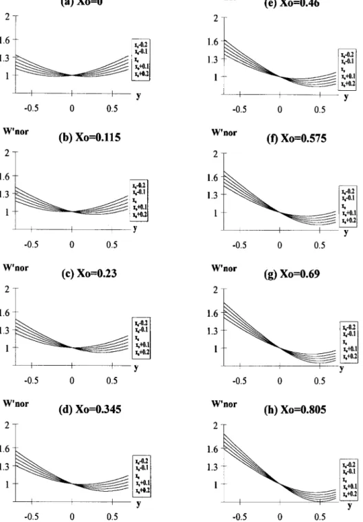
values so as to make the DOF optimum.The DOF calculation is very complicated as a function of two parameters ~x and y!. Within the flying region s0
2Ds<s<s01Ds, i.e., in the normalized form the region
x02Dx<x<x01Dx, there exists a ratio r of the maxi-mum to the minimaxi-mum output beam radii within the region y02Dy<y<y01Dy in the output space of the focusing lens. For any x0 value, there always exists an optimum y0
value that makes the beam radius ratior minimum. On the contrary, if an optimum y0 is chosen, the Dy should be
maximum for a fixed r value. The maximum Dy is the
increasedux0u for x0,0. Figure 5, given by Eq. ~4a! with
Dx50.2, shows the tendency that the less ux0u has the
larger DOF. This means that the DOF value decreases as the ux0u value increases. Therefore, the following analysis of the limited region ux0u<Dx is actually an optimum analysis of the DOF in flying optics.
5 DOF Determination in Flying Optics
Now, we explore the acceptable region of both the x and y variations in Eq.~4a!. To reduce the variation of beam ra-dius at lens, we limit the flying of s in the collimated region
2Zr<(s2 f )<Zr, i.e., 21<x<1. For y, we consider
that if the maximum variation ratio of beam radius after lens is taken to be r, from Eq. ~5a! we get s
8
2(r221)1/2Zr
8
<t<s8
1(r221)1/2Zr8
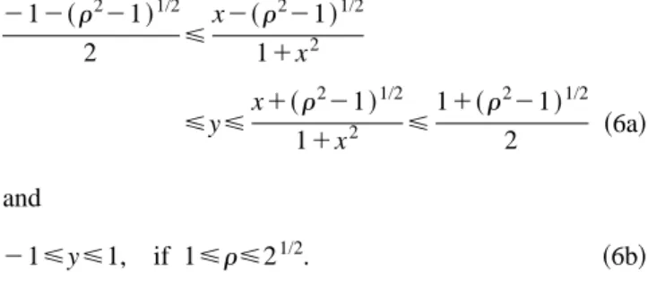
for every s value andhave 212~r221!1/2 2 < x2~r221!1/2 11x2 <y<x1~r 221!1/2 11x2 < 11~r221!1/2 2 ~6a! and 21<y<1, if 1<r<21/2. ~6b!
The focused beam radii at any plane in the region 21
<y<1, during flying region 21<x<1, are always inside
the region constrained by curves of xmin5x02Dx and xmax
5x01Dx. The reason can be expressed as follows.
Accord-ing to Eq.~4a!, the minimum wnor
8
occurs at x51/y if the y remains constant and a larger deviation from this x value causes larger wnor8
. Then, the absolute value of optimum x is always not less than one in the region21<y<1 and the largest absolute x value always has the minimum wnor8
dur-ing flydur-ing region21<x<1.Figure 6, given by Eq.~4b!, shows the variation of the focused beam radius as a function of y for a given positive value of x. The maximumDy, i.e., the DOF, occurs as the focusing point locates at the beam waist where y05x/(1
1x2). Once the focusing point shifts from beam waist, the
maximumr value within the region y02Dy<y<y01Dy occurs at y0ur max5 x 11x26
F
Dy 21 1 ~11x2!2G
1/2 . ~7!Here if 0<x<1, we can find that y0ur
max(minus root),0 or y0ur
max(plus root).2x/(11x
2). This means that within
the region y0ur
max(minus root)<y0<y0urmax(plus root) marked as region I in Fig. 6, if the focusing point comes closer to the beam waist, theDy value becomes larger. This
Fig. 4 Surface and contour of focused beam radius Wnor8 5@y2 1(xy21)2#1/2.
conclusion can also be available in the region y0ur
max(plus root)<y0<y0urmax(minus root) for 21<x
<0.
The DOF of flying optics for any flying region xmin<x
<xmax, where ux0u<Dx, xmin>21, xmax<1, can be deter-mined by the condition wnor
8
(xmax,ymin)[wnor8
(xmin,ymax)under which the beam radius ratio r within the region ymin<y<ymaxis minimum. The reason is expressed as fol-lows. In the case where ymax does not exceed the beam
waist position of xmax curve, i.e., ymax<yR, as shown in
Fig. 7~a!, an increasing y0 value causes the maximum and
minimum radii in the 2Dy region to move from A ~or Aa! and B to AR and BR, respectively, and the beam radius
ratiorincreases. Otherwise, decreasing y0value causes the
maximum and minimum radii in the 2Dy region to move from A ~or Aa! and B to AL and BL, respectively, and
according to the discussion on Fig. 6, the beam radius ratio
r still increases. In the case where ymax does exceed the
beam waist position of xmaxcurve, i.e., ymax.yR, as shown
in Fig. 7~b!, the minimum radius is at B, increasing or
decreasing the y0 value causes the maximum radius A to increase to AR or AL, respectively, and the beam radius ratior increases.
6 Derivative of the DOF in Flying Optics
With the flying range 2L, s varies within the region s0 2L<s<s01L, or 2L1( f 1d)<s<L1( f 1d), where
d[s02 f and 0<d<L, and then we have
21<x02Dx<x<x01Dx<1,
and
H
x05d/ZrDx5L/Zr . ~8!
The required region of y is
21<y02Dy<y<y01Dy<1,
where
H
y5~t2 f !Zr/~ f2! y05~t02 f !Zr/~ f2!Dy5~DOF!Zr/~ f2!. ~9!
On the xmin curve, the normalized waist radius is
wnor
8
~L!5F
1 11~xmin!2G
1/2 ~10! at the location yL5 xmin 11~xmin!2. ~11!On the xmaxcurve, the normalized waist radius is
wnor
8
~R!5F
1 11~xmax!2G
1/2 ~12! at the location yR5 xmax 11~xmax!2. ~13!The DOF is evaluated from point y50 where the wnor
8
re-mains constant when x varies as shown in Fig. 7.In the region y>0 (t> f ), the maximum wnor
8
locates on the xmincurve and the value increases with the y value.The minimum wnor
8
locates on the xmaxcurve, and the value decreases with the y value in the region 0<y<yR butin-creases with the y value in the region y.yR. Therefore, we get
max wnor
8
5$~ymax!21@~ymax!~xmin!21#2%1/2 ~14!min wnor
8
55
$~ymax!21@~ymax!~xmax!21#2%1/2
if 0<ymax<yR
F
1 11~xmax!2G
1/2 if ymax.yR. ~15!According to the requirement max wnor
8
/min wnor8
5r, we can calculate the ymax from the preceding equations andhave
Fig. 6 Variation of the focused beam radii (Wnor8 ) as a function ofy
for a given positive value ofx.
yt. f[~ymax!~Dx!
5
5
~r211!1~r221!a2@4r22~r221!2~1/Dx!2#1/2 ~r221!@~11a!21~1/Dx!2#14a
if Dx>Dxbp
2~12a!@~11a!21~1/Dx!2#1~~1/Dx!2@~11a!21~1/Dx!2#$~r221!@~11a!21~1/Dx!2#24r2a%!1/2 @~11a!21~1/Dx!2#@~1/Dx!21~12a!2# if Dx<Dxbp, ~16a! where
H
a5d/L Dx5L/Zr ~16b!Using the relationship yt. f(Dx5Dxbp)uDx>Dx(bp)[yt. f(Dx5Dxbp)uDx<Dx(bp)[(yR)(Dx) and Eq. ~16a! in which Dx
5Dxbp, we can find Dxbpas Dxbp5
S
@~r221!a212~r223!a1~r225!#1$@~r221!a212~r223!a1~r225!#2116~r221!~11a!2%1/2
8~11a!2
D
1/2
. ~17!
In the region y,0 (t, f ), we can calculate the yminwith the condition wnor
8
(xmax,ymin)[wnor8
(xmin,ymax) and have yt, f[~ymin!~Dx!5~11a!2~@~1/Dx!21~11a!2#$@~1/Dx!21~12a!2#y
t. f212~12a!yt. f%1~11a!2!1/2
~1/Dx!21~11a!2 ~18!
Therefore, the normalized DOF can be expressed as
DOFnor[~DOF!L
f2 5
yt.t2yt, f
2 . ~19!
The nominal focusing point, i.e., the center of the allowable region, has a position shift from the back focal point of lens. This shift can be normalized and expressed as
D fnor[~t02 f !Lf2 5
yt. f1yt, f
2 . ~20!
In the region2L<d<0, i.e., 2Dx<x0<0, with a simi-lar procedure the same result can be obtained except that
udu takes place of d andD fnorchanges its sign.
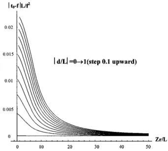
Figures 8 and 9, given by the Eqs.~19! and ~20!, show the variations of DOFnorandD fnor. From these figures, it
can be seen that the left-side start point of each curve with differentudu/L value is different. The reason is that present analysis has the limited region 21<x<1, i.e., 1/Dx>1
1ux0u/Dx. Because 1/Dx[Zr/L and ux0u/Dx[udu/L, we
Fig. 8 System DOF of flying optics as a function ofZrandd.
Fig. 9 System focusing point shift of flying optics as a function ofZr
find the condition Zr>L1udu. We can find the conditions for the optimal DOF of flying optics as follows:
1. An optimum Zr should be taken.
2. The center of flying region should locate at front fo-cal point (d→0).
3. The lens of longer focal length should be used. 4. Less value in flying range (2L) should be taken. 7 Flying Optics withd50
In case of d50, i.e., a50, the 1/e2 radius curves are sym-metrical with respect to the t5 f plane @x050, see Fig. 5~a!#. From Eqs. ~16a! and ~18!, we have
yt. f52yt, f5
5
~r211!2@4r22~r221!2~1/Dx!2#1/2 ~r221!@11~1/Dx!2# if Dx>Dxbp 211~r221!1/2~1/Dx! 11~1/Dx!2 if Dx<Dxbp. ~21!From Eq.~21!, we have the optimal results as
H
Dxuopt5S
r21 r11D
1/2 DOFnoruopt5r21 2 . ~23!In laser material processing, if we take r51.1 and d50, from Eq. ~23!, the optimal condition of input beam is Zr5
A
21L and the optimum DOF is 0.05f2/L.8 Analysis Example
To demonstrate the use of our derived equations, an ex-ample is presented of the optimum design of output coupler in laser-gantry-robot systems. The system geometry is shown in Fig. 10, which consists of a stable resonator with R15`, R2530 m, L058.05 m, a focusing lens with f1 50.254 m, and flying optics with L56 m. The curvature
radius R3 of the outside surface in this output coupler is
considered as a variable to find the optimum DOF value for
r51.1.
Following Luxon’s analytical approach,5 the focal length of output coupler was modified for the thermal-lensing effect with the equation 1/fT51/f011/fther, in
which fther583.9 m, see Figs. 11~a! and 11~b!. The output beam parameters (s0
8
,Zr08
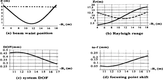
) of the laser resonator as the functions of the radius R3, are shown in Figs. 11~c! and11~d!. In this system where the flying region is from 4 to 16 m after the output coupler, the center of the flying region is at the position L1510 m. The output beam parameters of
Fig. 10 Geometry of the flying optics.
Fig. 11 Optimizing the output coupler (R15`, R2530 m, L058.05 m, fther583.9 m, and
nZnSe(lco
2)52.4) and output beam parameters (s08,Zr08) of laser resonator as the functions ofR3,
the laser resonator should be transferred to the input beam parameters (d,Zr) of flying optics with d5(L12s0
8
)2 f1and Zr5Zr15Zr0
8
. Figures 12~a! and 12~b! show d and Zr as functions of R3, respectively. According to ouras-sumptions 21<x<1 and 2Dx<x0<Dx, we have the constraints Zr>L1udu and udu<L, as the dashed curves show in these figures, which limit the considered region of R3. Then using Eqs.~19! and ~20!, we calculate the DOF
and focusing point shift shown in Figs. 12~c! and 12~d! in which the optimum DOF is about 0.47 mm when R35
211.5 m. If R35217 m is chosen, we get DOF>0.29
mm, which is shorter. Figure 13 shows that R35211.5 m has larger variations in output beam parameters (s1
8
,Zr18
)of focusing lens during flying, but with a larger Zr1
8
value,which results in a larger DOF.
This example shows that we can not get the optimum DOF of flying optics only by minimizing the variations of w0
8
, Zr8
, and s8
.9 Discussion and Conclusions
In laser material processing the power density~irradiance! of working beam has a tolerance range for a particular ap-plication. As a fixed laser power is applied during process-ing, this tolerance becomes a constraint on the acceptable variation in the working beam radius. Because the ma-chined materials do have a certain thickness, the DOF of
Fig. 12 Optimizing the output coupler (flying region 4, 16 m; 10-in. focusing lens,r51.1) and focusing beam parameters (system DOF, focusing point shift) as functions ofR3, respectively. The dashed lines in (a) and (b) are drawn by the equationsudu5LandZr5L1udu, respectively.
Fig. 13 Optimizing the output coupler: the variations of focus and DOF forR35217 m and R3
shown in Figs. 3, 4, and 5, makes the DOF analysis diffi-cult. The maximum value of the DOF requires both the fewer variations of w0
8
, Zr8
, and s8
and a larger Zr8
value at the same time. From Fig. 3, fewer variations of w08
and Zr8
requires a larger Zr/ f value and s0→ f , but lessvaria-tion of s
8
requires a larger Zr/ f value and s0→ f 6Zr.However, the larger Zr
8
requires a smaller Zr/ f value. In earlier works, these inconsistent requirements made it dif-ficult to find the optimal DOF value and associated param-eters in system design. In this paper, the total effect of these parameters on the flying optics are derived and explicitly shown in Fig. 8. The DOF of flying optics can be evaluated with Eq.~19! as a merit function to give the optimal system parameters (d,Zr) and the optimal DOF itself. In the non-flying optics, as discussed in the preceding section, a mini-mum Zr value is required when optimini-mum condition s5 f are taken.In the laser material processing system design, both the working beam radius and the DOF must be considered. In this paper, the DOF analysis in flying optics can be used to optimize the DOF during the system design.
Acknowledgments
This work was supported by the National Science Council under the grant No. NSC-85-2215-E-009-004 and by the Mechanical Industry Research Laboratories of the Indus-trial Technology Research Institute of the Republic of China.
References
1. H. W. Kogelnik and T. Li, ‘‘Laser beam and resonators,’’ Appl. Opt. 5~10!, 1550–1567 ~1966!.
5. J. T. Luxon, ‘‘Optical calculations for a laser-gantry-robot system,’’ in Proc. ICALEO’87, pp. 85–90~1987!.
6. U. Zoske and A. Giesen, ‘‘Optimization of the beam parameters of focusing optics,’’ in Proc. 5th Int. Conf. Laser in Manufacturing, pp. 267–278~1988!.
7. H. Haferkamp, H. Schmidt, and D. Seebaum, ‘‘Beam delivery using adaptive optics for material processing applications with high power CO2laser,’’ Proc. SPIE 2062, 61–68~1993!.
Chih-Han Fang received his BS degree
from National Cheng-Kung University in 1980 and the MS degree from National Chiao-Tung University in 1985. Currently, he is pursuing a PhD at the Institute of Electro-optical Engineering, National Chiao-Tung University. He has been a re-searcher in optical system design of power laser machines for material processing at the Mechanical Industrial Research Labo-ratories, Industrial Technology Research Institute, since 1985.
Mao-Hong Lu graduated from the
De-partment of Physics at Fudan University in 1962. He then worked as a research staff member at the Shanghai Institute of Phys-ics and Technology, Chinese Academy of Sciences, from 1962 to 1970, and at the Shanghai Institute of Laser Technology from 1970 to 1980. He studied at the Uni-versity of Arizona as a visiting scholar from 1980 to 1982. He is currently a professor at the Institute of Electro-optical Engineer-ing, National Chiao-Tung University.