反應擴散方程在移動曲面上的數值模擬

國立交通大學

應用數學系

碩 士 論 文

反應擴散方程在移動曲面上的數值模擬

Numerical Simulations of the Reaction-Diffusion

Equation on the Moving Surface

研 究 生：陳建明

指導教授：賴明治 教授

反應擴散方程在移動曲面上的數值模擬

Numerical Simulations of the Reaction-Diffusion

Equation on the Moving Surface

研 究 生 : 陳建明 Student: Chien-Ming Chen

指導教授 : 賴明治 Advisor: Ming-Chih Lai

國 立 交 通 大 學 應 用 數 學 系

碩 士 論 文 A Thesis

Submitted to Department of Applied Mathematics College of Science

National Chiao Tung University in Partial Fulfillment of the Requirements

for the Degree of Master

in

Applied Mathematics July 2008

Hsinchu, Taiwan, Republic of China

i

反應擴散方程在移動曲面上的數值模擬

學生 : 陳建明 指導教授 : 賴明治 教授 國立交通大學應用數學系(研究所)碩士班 摘 要 這篇論文的主要目的是使用快速傅立葉轉換的優點來數值上地解反應擴散方程組， 並且解以移動的曲面為定義域的方程組。在未來的工作上希望能夠找出近似心臟的舒張 與收縮的移動曲面方程式以結合反應擴散方程式來做出更好的心臟電流傳導的數值模 擬。首先，在球面座標與橢球面座標下利用譜方法和一些二階精確的數值方法分別做球 面上及橢球面上的熱方程快速解法。接著，使用這兩種快速解法並且結合時間分解的方 式產生反應擴散方程的快速解法。再來，使用在曲線座標下的曲面拉普拉斯算子來數值 上地解熱方程，利用這個數值解可以計算定義在移動曲面上的熱方程，進一步用它來計 算傳導擴散方程。在以上的各種數值解下，我們皆舉了四個可以涵蓋其他各種情形的例 子去觀察質量的變化。最後，對這些數值解和質量的變化我們做出了結論及它們的應用 性。

ii

Numerical Simulations of the Reaction-Diffusion

Equation on the Moving Surface

Student：Chien-Ming Chen

Advisor：Dr.Ming-Chih Lai

Department(Institute) of Applied Mathematics National Chiao Tung University

ABSTRACT

The central objective of this thesis is to use the fast fourier transform to numerically solve the reaction-diffusion systems and solve another systems whose domain moves with time. Hope that we could produce the equations on the moving domain which approximates the diastole and systole in human hearts. First, use the spectral method and some second-order numerical methods to produce the fast heat solvers on the spherical and ellipsoid surface domain in spherical coordinates and ellipsoid coordinates, respectively. Then, couple these two fast solvers with the time splitting method to produce the fast solver of the reaction-diffusion equation. Next, we use the surface Laplacian operator in Curvilinear coordinates to numerically compute the heat equation. Therefore, this heat solver could compute the heat equation on the moving surface domain. Furthermore, use it to compute the convection-diffusion equation. In each of above numerical solvers, we give four examples which could cover other situations to observe the changes in the mass. Finally, we summarize the applications and results for these numerical solvers and changes in the mass.

iii

誌 謝

這篇論文的完成，首先，我最需要感謝的是我的恩師，也就是我的指導教授賴明治 教授。在老師的循循善誘下，我漸漸懂得數學在應用方面的實用性及重要性，對自己在 學習的路上無疑是添加了強心劑，在作研究的過程中，不僅學會了許多數值計算的方法 與實作，在科學計算上又有更深的了解；在每週的 meeting 裡，我學到的不僅僅是做研 究的方法，還有做研究的態度，更重要的是做人處事的道理，在研究上他更是會替我們 指引方向，在研究中的這片汪洋大海裡，老師有如指南針般讓我們不會在裡頭迷失自己 要走的路，老師對我的重要性更是不言而喻。 在研究所這兩年裡，我要感謝曾昱豪與陳冠羽學長和曾孝捷學長，在我對研究與程 式上遇到挫折、感到灰心、受到打擊時，有學長的聊天交流與學業和研究上的指點，其 中得到的關懷讓我又對研究產生了許多衝勁，學長在我對研究的路上也指導了我許多正 確的方向也給了我一些他的經驗法則，讓我在瓶頸中得到了許多啟發。 我要感謝 308 實驗室的所有室友(同學)，在平常的聚會或聊天中，有時都會聊到彼 此研究的東西，互相以不同的角度來思考，說出自己的想法，這樣的實驗室讓我學習到 team 的重要，以及由 team 感受到大家用心在研究上的氣氛，對我這兩年的研究生活也 添加了許多動力和想法，其中尤其是我的室友謝先皓，在我剛踏入交大應數所的研究之 旅時，他以在交大應數系時的豐富經驗與數學知識給予我在研究與課業上許多的幫助， 是個非常好的研究搭檔。 我要感謝吳恭儉學長，在我 PDE 方面學識較不足的地方以及對課業產生困惑的地方， 總是有他可以讓我請教，並從中獲取新的 idea。 我要感謝蔡明誠、李金龍與李信儀學長，在一年級的必修實變數函數論中，學長們 會不吝惜自己的時間願意讓我與他討論課業上的問題，面對我的問題，他們總是不厭其 煩的指導我，不管犧牲了多少學長自己的時間，他們都是一樣熱心，感謝學長的熱誠與 用心，讓我能在有著必修壓力的碩一生活能順利度過，也感受到研究生活中令人感到相 當溫暖的一面。 研究所的路上，還有著許多的學長姐與學弟妹溫暖的關心，像芳婷、蕙蘭、康伶學 姐與喻培、明耀、文貴、育豪、川和學長與仁洲、裕昇、振庭學弟和實驗室的學弟們都 是我能快樂享受研究的來源之一，讓我感受到作研究的我並不孤單。 再來，我要特別感謝的是這次擔任口試的委員王偉仲教授、黃聰明教授、吳金典教 授，謝謝他們花費心思檢視我的論文，並且給予我的論文許多有益的建議，讓我的論文 更趨完整。 最後，我感謝我的父母能夠讓我在這樣的研究所生涯裡，全力的去唸書與研究，不 用去顧及其他事物的煩惱，以致於我能夠順利的畢業，沒有他們和女友怡玲的關心與期 待，我將無法擁有這樣的動力與使命感去完成我的學業。也感謝所有關心我的人，在這 裡與您一起分享此篇論文的喜悅。

iv

目

錄

中文提要

………

i

英文提要

………

ii

誌謝

………

iii

目錄

………

iv

1、

Introduction ………

1

2、

Numerical Scheme ………

2

2.1

Fast Fourier Transform ………

2

2.1.1 Fourier Transform ………

3

2.1.2 Discrete Fourier Transform ………

3

2.1.3 Fast Fourier Transform ………

6

2.2

Second-Order Finite Difference Method ………

7

2.2.1 Second-Order Central Difference Method ………

7

2.2.2 Second-Order Symmetric Discretization ………

8

2.3

Second-Order Crank-Nicolson Method ………

10

2.4

Thomas Algorithm ………

10

3、

Fast Heat Solver in Spherical Coordinates ………

12

3.1

Heat Solver on a Spherical Surface Domain ………

12

3.1.1 Abstract ………

12

3.1.2 Solvers with the Central Difference Method ………

13

3.1.3 Solvers with the Symmetric Discretization ………

20

3.2

Numerical Results ………

24

3.2.1 Results of Solvers with the Central Difference Method ……

24

3.2.2 Results of Solvers with the Symmetric Discretization………

25

3.3

Mass Conservation ………

26

3.3.1 The Mass of Solvers with the Central Difference Method …

27

3.3.2 The Mass of Solvers with the Symmetric Discretization ……

33

3.3.3 Comparison between the Central Difference Method and

the Symmetric Discretization in Spherical Coordinates ……

38

4、

Fast Heat Solver in Ellipsoid Coordinates ………

39

4.1

Heat Solver on an Ellipsoid Surface Domain ………

39

4.1.1 Solvers with the Central Difference Method………

39

4.1.2 Solvers with the Symmetric Discretization ………

42

4.2

Numerical Results………

46

4.2.1 Results of Solvers with the Central Difference Method………

46

4.2.2 Results of Solvers with the Symmetric Discretization ………

47

v

4.3.1 The Mass of Solvers with the Central Difference Method …

49

4.3.2 The Mass of Solvers with the Symmetric Discretization ……

56

4.3.3 Comparison between the Central Difference Method and the

Symmetric Discretization in Ellipsoid Coordinates …………

60

4.3.4 Comparison between Chapter 3 and Chapter 4 ………

61

5、

The Primary Cardiac Simulation of Human Beings …………

62

5.1

The Reaction-Diffusion Equation………

62

5.2

Numerical Methods and Techniques………

63

5.2.1 Gilbert Strang Splitting Method………

63

5.2.2 Numerical Techniques ………

64

5.3

Numerical Solvers ………

65

5.3.1 Numerical Solver of the Reaction-Diffusion Equation on a

Spherical Surface Domain ………

65

5.3.2 Numerical Solver of the Reaction-Diffusion Equation on an

Ellipsoid Surface Domain ………

66

5.4

Results and Analysis ………

67

5.4.1 Numerical Results of the Reaction-Diffusion Equation on a

Spherical Surface Domain with R=16 ………

68

5.4.2 Numerical Results of the Reaction-Diffusion Equation on an

Ellipsoid Surface Domain which Approximates to R=16……

69

5.4.3 Numerical Results of the Reaction-Diffusion Equation on an

Ellipsoid Surface Domain which Approximates to Cardiac

Size ………

70

6、

Explicit Numerical Solver of the Heat Equation ………

74

6.1

Discretization of the Heat Equation ………

74

6.2

Results of the Explicit Numerical Solvers for the Heat

Equation ………

80

6.2.1 Test Accuracy of the Solvers ………

80

6.3

Mass conservation………

81

6.3.1 The Mass of the Solver with Section 6.1 and Central

Difference Method 1………

83

6.3.2 The Mass of the Solver with Section 6.1 and Central

Difference Method 2………

87

6.4

Comparison ………

92

7、

Numerical Solver of the Convection-Diffusion Equation ……

92

7.1

Discretization of the Convection-Diffusion Equation ………

92

7.2

Results of the Convection-Diffusion Equation on the Moving

Surface………

94

8、

Applications ………

100

vi

1

1、Introduction

Modeling is an imperative headway in science and numerical simulations stringing along with it. Both of them play the important roles in our modern livelihood. The reason is that the numerical simulations always help people to discover something amazing. For examples, they could be used to predict, test or find some rules, etc. In many applications of them, we concentrate on predicting the motions of waves. Propagation of waves has been appeared in many behaviors of biological and chemical experiments. Mathematical modeling can uphold and connect with these experiences. Because the electrical activities of the human hearts can be modeled by the nonlinear reaction-diffusion (RD) equations [15] and the FitzHugh -Nagumo-type model on the spherical surface domain with fixed radius has been simulated in [6], we are attracted to these related problems. In recent years, there are many kinds of cardiovascular diseases which our world replete with. We are anxious to develop some numerical simulations that are concerned with the electrical activities of our hearts to help treating the cardiopathy and anticipating obtaining some things good for the medical treatment of human beings. But these are our final expectations and goals. According to the developments of the present techniques of modeling, we only expect to use the forthcoming model in [6] to develop a mathematical basis for understanding the propagation of electrochemical waves in human hearts.

Here make mention of [6] in brief. The authors administered the simulation of the reaction-diffusion systems on a spherical surface domain with a radius r ∈ 11,16 to perform circular waves by beginning with some initial values and regulating some parameters of the systems. These numerical results came into being meandering of spiral waves. Next, we are going to simulate the reaction-diffusion equation on a spherical surface domain with a radius r = 16 as [6] and simulate it on an ellipsoid surface domain whose size is close to a spherical surface with r = 16 and simulate it on an ellipsoid surface domain whose size is

2

close to realistic cardiac in Chapter 5. Before performing our works, the numerical schemes in Chapter 2 are essential to our simulations. In Chapter 3, we solve the heat equation implicitly on a spherical surface domain in spherical coordinates with the schemes in Chapter 2 for Chapter 5. In Chapter 4, we solve the heat equation implicitly on an ellipsoid surface domain in ellipsoid coordinates with the schemes in Chapter 2 for Chapter 5. After solving the reaction-diffusion systems in Chapter 5 to simulate the propagation of electrochemical waves in human hearts, we expect to see how the propagation of electrochemical waves proceeds on the moving surface. Now, reduce this problem to solve the convection-diffusion equation (We will introduce this in Chapter 7.) on the moving domain. It is reasonable to solve the heat equation before solving the convection-diffusion equation. We solve the heat equation in Curvilinear coordinates in place of solving it in spherical or ellipsoid coordinates as Chapter 3 and Chapter 4 because the domain moves with time. And impose the explicit schemes on the solver because it is easy to find that we must extra define the values on the north and south poles head-on when using implicit schemes on it. Due to above reasons, we solve the heat equation in Curvilinear coordinates with the explicit schemes and check out this solver in Chapter 6. Therefore, we could solve the convection-diffusion equation in Chapter 7 with the discretization of Chapter 6. In the end, our future works are that combine the techniques in Chapter 7 with the reaction-diffusion systems whose domain approximates to human hearts. Expect to produce a primary and more real-life cardiac simulation of human beings. By the way, we are interested in observing if the total mass complies with the mass conservation law in each of our numerical solvers.

2、Numerical Scheme

2.1 Fast Fourier Transform

Before talking about the fast Fourier transform (FFT), we introduce the Fourier Transform and the discrete Fourier transform (DFT). We will use the FFT to discrete our

3

spatial terms which is periodic in our equation. The contents in this section come from [14].

2.1.1 Fourier Transform

Transform u(x) into Fourier series formula, then we get u x = n_k=0a_kϕ_k(x),

where ak are constants, ϕk x = eikx, x ∈ 0,2π , f, g = f(x)g(x)₀2π dx means inner

product. Theorem: If f ∈ L2 0,2π = f ∶ 0,2π → ℂ f(x) ₀2π 2dx < ∞ , then f(x) = ∞_k=−∞f _keikx, f =_k 1 2π f(x)e −ikx_dx 2π 0 . (1)

Here f _k is called continuous Fourier coefficient, and we have the properties:

𝐟 𝐱 = f k𝐞𝐢𝐤𝐱 ∞ 𝐤=−∞ 𝐟(𝐱) = 𝐟 _k𝐞−𝐢𝐤𝐱 ∞ 𝐤=−∞ => 𝐟(𝐱) = f −k𝐞−𝐢𝐤𝐱 ∞ −𝐤=−∞ 𝐟(𝐱) = 𝐟 _k𝐞−𝐢𝐤𝐱 ∞ 𝐤=−∞ => f _−k = 𝐟 _k (2)

2.1.2 Discrete Fourier Transform

Discrete f, g = f(x)g(x)₀2π dx by trapezoid rule and cut 0,2π into N partitions uniformly. Then derive f, g _N = h N−1f(x_j)g(x _j)

j=0 , where h =2π_N. Here mesh the

grids as follows:

4 f x ≡ f _keikx N 2−1 k=−N₂ , f _k = 1 N f(xj)e−ikxj N−1 j=0

where x_j = jh = j2π_N, f _k is called discrete Fourier coefficient, f depends on N because f

was cut into N partitions. So, call into being the formulation:

It is easy to know f x_j = f_j = f _keikxj N 2−1 k=−N₂ , j = 1, 2, … , N − 1. (3)

In order to make the indices be the same with 0, 1, … , N − 1, we show it in below contents: Let d_k ≡ f _k−N 2 = 1 N fje −i(k− N_2)xj N−1 j=0 = 1 N (fje iN_2xj_)e−ikxj N−1 j=0 Fj ≡ fjeiN2xj (4) We derived dk = 1 N (Fj)e−ikxj N−1 j=0 , for k = 0, 1, … , N − 1. Substitute (3) into (4), F_j ≡ f_jeiN2xj _{= f} kei k+N2 xj = N 2−1 k=−N₂ f k−N₂e ikxj = N−1 k=0 d_keikxj N−1 k=0 , for j = 0, 1, … , N − 1.

5 dk = _N1 N−1j=0 Fje−ikxj

Fj = N−1k=0dkeikxj

, k = 0 , 1 , … , N − 1._{, j = 0 , 1 , … , N − 1.} and the formulation:

In the configuration of matrix, the definition says d0 d1 d2 ⋮ dN−1 = 1 N ω0 _ω0 _ω0 _{⋯ ω}0 ω0 _ω1 _ω2 _{⋯ ω}N−1 ω0 ω0 ⋮ ω0 ω2 ω3 ⋮ ωN−1 ω4 ω6 ⋮ ω2 N−1 ⋯ ⋯ ⋯ ω2 N−1 ω3 N−1 ⋮ ω N−1 2 F0 F₁ F2 ⋮ FN−1 (5) where ω = e−i 2π N .

The N × N matrix in (5) is called the Fourier matrix,

HN ≡ 1 N ω0 _ω0 _ω0 _{⋯ ω}0 ω0 _ω1 _ω2 _{⋯ ω}N−1 ω0 ω0 ⋮ ω0 ω2 ω3 ⋮ ωN−1 ω4 ω6 ⋮ ω2(N−1) ⋯ ⋯ ⋯ ω2(N−1) ω3(N−1) ⋮ ω(N−1)2

Here H_N is a symmetric matrix, and the Fourier matrix has an inverse matrix:

H_N−1 = ω0 _ω0 _ω0 _{⋯ ω}0 ω0 _ω−1 _{ω−2 ⋯ ω−(N−1)} ω0 ω0 ⋮ ω0 ω−2 ω−3 ⋮ ω−(N−1) ω−4 ω−6 ⋮ ω−2(N−1) ⋯ ⋯ ⋯ ω−2(N−1) ω−3(N−1) ⋮ ω−(N−1)2

Now, we have the forward Fourier transform

H_N F0 F₁ F2 ⋮ FN−1 = d0 d1 d2 ⋮ dN−1

6 HN−1 d₀ d₁ d₂ ⋮ d_N−1 = F₀ F1 F₂ ⋮ F_N−1 , where H_N−1 _{= H} N .

2.1.3 Fast Fourier Transform

The discrete Fourier transform that we used in the traditional way needs O N2 operations. Cooley and Tukey [4] could achieve the DFT in O N log N operations in an algorithm which called the fast Fourier transform (FFT) which takes advantage of divide and conquer algorithm. We can write the DFT (5) as

d = d₀ d₁ d₂ ⋮ d_N−1 = 1 NGN F₀ F1 F₂ ⋮ F_N−1 = 1 NGNF where G_N = ω0 _ω0 _{ω0 ⋯ ω0} ω0 _ω1 _ω2 _{⋯ ω}N−1 ω0 ω0 ⋮ ω0 ω2 ω3 ⋮ ωN−1 ω4 ω6 ⋮ ω2(N−1) ⋯ ⋯ ⋯ ω2(N−1) ω3(N−1) ⋮ ω(N−1)2 , F = F0 F₁ F2 ⋮ FN−1 .

We will show how to compute b = G_NF recursively. It needs to divide by N to complete the

DFT because d =_Nb. In the beginning, we show how the n = N case works. FFT takes the

advantages of G_N and GN 2

. Let M =N

2, and our indices of matrix are taken as Fortran form.

b = G_NF, ω_N = e−i2πN _{and suppose} N is even here ( If N is odd, then the process is similar

with that we discuss here. ). Then

b_j = (G_NF)_j = ω_NjkF_k N−1 k=0 = ω_NjkF_k N−2 k=0 k∈even + ω_NjkF_k N−1 k=1 k∈odd

Substitute M =N₂, ℓ =k₂ and ω_M = e−i

2π

7 b_j = ω_Nj2ℓF_2ℓ M−1 ℓ=0 + ω_Nj 2ℓ+1 F_2ℓ+1 M−1 ℓ=0 = ω_MjℓF_2ℓ M−1 ℓ=0 + ω_Nj ω_MjℓF_2ℓ+1 M−1 ℓ=0

In summary, the calculation of the DFT(N) can be performed by computing a pair of DFT(N₂)s

and some extra multiplications and additions. Consider n, ignore the 1_n temporarily, DFT(n)

can be reduced to a pair of DFT(n

2)s plus O n extra operations which are multiplications

and additions. We use above idea recursively and this is the most important techniques to make DFT solver more fast. Let n be a power of 2. Then the Fast Fourier Transform of size n can be accomplished in n 2 log₂n − 1 + 1 additions and multiplications, plus a division

by n [14]. We use the FFT to help computing our numerical solutions. And it leads to less computation by reducing O N2 operations to O N log₂N operations.

2.2 Second-Order Finite Difference Method

We will use Section 2.2.1 and Section 2.2.2 numerical methods to discrete our spatial terms of our equations.

2.2.1 Second-Order Central Difference Method

We refer to [14] to make this section complete. As below saying:

Let y be the function which depends on x. x_i is the interior mesh point, for i = 1 , 2, … , N. and x_i+1− x_i = h. Expanding y in a third Taylor polynomial at x_i to evaluate y at x_i+1 and x_i−1, then we have

y x_i+1 = y x_i+ h = y x_i + hy′ _x i + h2 2 y′′ xi + h3 6 y′′′ xi + h4 24y 4 ξi+ (6) for some ξ_i+ in x_i, x_i+1 , and

y xi−1 = y xi− h = y xi − hy′ xi + h2 2 y′′ xi − h3 6 y′′′ xi + h4 24y(4) ξi − ₍₇₎

8

for some ξ_i− in x_i−1, x_i , and assume y ∈ ∁4 x_i−1, x_i+1 here.

If subtract (7) from (6), then the terms involve y′′ x_i and y(4) x_i are eliminated. y′ _x

i =

1

2h y xi+1 − y xi−1 − h2

6 y′′′ ηi , for some ηi in xi−1, xi+1 . Therefore,

y′ _x i ≈

1

2h y xi+1 − y xi−1 + O h2 (8) Use the same techniques, we could also have

y′ _x i ≈

1

h y xi+12 − y xi−12 + O h

2 ₍₉₎

If add (6) to (7), then the terms involve y′ x_i and y′′′ x_i are eliminated. y′_{′ x} i = 1 h2 y xi+1 − 2y xi + y xi−1 − h2 24 y(4)(ξi + ) + y 4 _(ξ i−) .

The Intermediate Value Theorem can be used in above equation： y′_{′ x}

i =

1

h2 y xi+1 − 2y xi + y xi−1 −

h2

12y 4 ξi , for some ξi in xi−1, xi+1 Therefore,

y′_{′ x} i ≈

1

h2 y xi+1 − 2y xi + y xi−1 + O h2 (10)

(8) (9) both are called central difference method for y′ _x i .

(8) denotes central difference method 1 in our paper here. (9) denotes central difference method 2 in our paper here. (10) is called central difference formula for y′_{′ x}

i .

They really have second-order accuracy.

2.2.2 Second-Order Symmetric Discretization

According to second-order accuracy of Section 2.2.1, we could produce a numerical method which was called Symmetric Discretization. This method builds up from the second-order central difference method. The progress of the symmetric discretization is as follows:

9

Step 1: We use the central difference method 2 for the whole f(xi)∂g(x_∂xi) as Figure 1.

Figure 1 ∂ ∂x(f(xi) ∂g(x_i) ∂x ) = f(x i+12) ∂g(x i+12) ∂x − f(x_i−12) ∂g(x i−12) ∂x ∆x

Step 2: We use the central difference method 2 for

∂g(x i+1₂) ∂x and ∂g(x i−1₂) ∂x as Figure 2. Figure 2 ∂g(x i+12) ∂x = g(x_i+1) − g(x_i) ∆x , ∂g(x i−12) ∂x = g(x_i) − g(x_i−1) ∆x

Step 3: After substituting Step 2 into Step 1, we will get the symmetric discretization as follows. ∂ ∂x(f(xi) ∂g(x_i) ∂x ) = f(x) i+12 g(x_i+1) − g(x_i) ∆x − f(x)_i−12g(xi) − g(x∆x i−1) ∆x

Because of second-order accuracy in Step 1 and Step 2, we have second-order accuracy on the symmetric discretization.

10

2.3 Second-Order Crank-Nicolson Method

We will use the numerical methods in this section to discrete our spatiotemporal terms of our equations. The Crank-Nicolson method is unconditionally stable and has order of convergence O(∆x2+ ∆t2) can be found in Isaacson and Keller [9]. According to [5], when we integrating the o.d.e.

u′ _{t = f( t , u t )}

on the interval I_n = [t_n, t_n+1], we could have

u t_n+1 − u t_n = f s, u s

tn +1

tn

ds = I_n (11)

Here we ignore spatial terms in u, i.e. the temporal terms dominate the accuracy. If we approximate the interval I_n, then we can compute u t_n+1 from the old value u t_n . The trapezoid rule

I_n ≈∆t

2 [f tn, un + f(tn+1, un+1)]

is used to estimate the integral (11). Here ∆t = t_n+1− t_n, un = u t_n . Consequently, we derive the formula of the Crank-Nicolson method:

u tn+1 − u tn ∆t = [f tn, un + f(tn+1, un+1)] 2 (12) From (9), we have u′ _t n+12 ≈ u t_n+1 − u t_n ∆t + O h2 (13) Take Taylor expansion for f t_n, un and f(t_n+1, un+1) at f(t_n+1

2, u

n+1_{2) and add each other}

similar to Section 2.2.1. Lastly, after combining with (13) we could have second-order accuracy on the Crank-Nicolson method.

2.4 Thomas Algorithm

In our numerical solvers, the most important procedure which saves our time and moves up our efficiency of computation is the method to solve the linear systems. Because the

11

linear systems that we need to solve almost belong to tridiagonal systems, here we introduce the tridiagonal matrix algorithm (TDMA) which is known as the Thomas algorithm. The systems can be described as follows:

i.e. AX = B

There are n unknowns as X. The Thomas algorithm is a correction of the LU decomposition idea to solve linear systems with three bands diagonal coefficient matrix. We show our programming in our solver in MATLAB as follows:

%==============THOMAS ALGORITHM================================ for k=2:n m=A(k,k-1)/A(k-1,k-1); A(k,k)=A(k,k)-m*A(k-1,k); B(k)=B(k)-m*B(k-1); end X(M)=B(M)/A(M,M); k=n-1; while k>=1 X(k)=(X(k)-A(k,k+1)*X(k+1))/A(k,k); k=k-1; end %============================================================= It is easy to know that the solution can be obtained in 0(n) operations instead of 0(n3) by using the Gaussian elimination. After this section, we have enough numerical methods to proceed with our numerical solutions.

1 1 1 1 2 2 2 2 2 1 1 1 1 1

.

0

.

.

.

.

.

.

.

0

.

n n n n n n n n n

b

c

x

d

a

b

c

x

d

a

b

c

x

d

a

b

x

d

    



 

 





 

 





 

 





 

 







 

 





 

 





 

 





 

 



12

3、Fast Heat Solver in Spherical Coordinates

3.1 Heat Solver on a Spherical Surface Domain

3.1.1 Abstract

The solution of the heat equation on a spherical surface geometry has many applications in the areas of biology, geophysics, and engineering. We will present a simple and efficient method which is FFT fast direct solver for Heat equation on a spherical surface domain. These solvers on the truncated Fourier series expansion, and the Fourier coefficients are solved by second-order finite difference methods. Let the grids of the north and south poles shift half a grid away from the poles [12] (We will show the architecture of the grids later.). Next, combine the symmetry constraint of the Fourier coefficients in the solver (We need not use the symmetry constraint in the solver with the symmetric discretization.). Hence we could deal with the coordinate singularities easily without the conditions of the south and north poles. The process of FFT only takes O(N log₂N) computations. After solving Fourier coefficients M times at the beginning and the end, the total operations of our solver only need O(MN log₂N) arithmetic operations for M × N grid points. The total cost here does not include solving the linear systems of the unknown Fourier coefficients N times. We derive these unknowns by solving the linear systems whose matrices are M × M and tridiagonal N times by Thomas algorithm which costs O(M) operations. If we impose (2) on our solver, then we only need to solve the linear systems N₂ times. Therefore, our solver

needs O(MN) arithmetic operations to solve these linear systems. All cost in our fast Heat solver needs only O(MN log₂N) operations (M and N will be introduced later.). We will know that it is convenient to rewrite the equations in spherical and ellipsoid coordinates in Chapter 3 and Chapter 4, respectively.

13

3.1.2 Solvers with the Central Difference Method

According to [6], we have the formula of the heat equation on a spherical surface domain in spherical coordinates as

u_t = ∆_su ∆_su = ∇_s2_{u =} 1 r2 ∂2_u ∂ϕ2+ cot ϕ ∂u ∂ϕ+ 1 sin2 _ϕ ∂2_u ∂θ2 (14) We also can derive the surface Laplacian term of (14) by [10] and set radius r be a constant R at the same time or by [16]

∇s2u = ∇2u −

∂2_u

∂𝐧2− κ

∂u

∂𝐧 (15) Here 𝐧 = r：normal, κ =2_r：mean curvature, x = Rsinϕcosθ, y = Rsinϕsinθ, z = Rcosϕ

in spherical coordinates, and ∆u = ∇2_{u =}∂2u ∂r2 + 2 r ∂u ∂r + 1 r2 ∂2_u ∂ϕ2+ cot ϕ ∂u ∂ϕ+ 1 sin2 _ϕ ∂2_u ∂θ2 (16)

comes from [10]. After replacing n = r and κ =2_r in 15 and substituting (16) into (15). In (14), ignore r by setting r a constant R, and denote u R, ϕ, θ, t ≈ u ϕ, θ, t .

0 ≤ ϕ < 𝜋 represent the directions of latitude, 0 ≤ θ < 2𝜋 represent the directions of longitude.

(14) was discreted by cutting the space as the following uniform grids which shift half a grid away from the poles.

14 Given any N = 2M, ∆ϕ =_Mπ = ∆θ = 2π_N,

ϕ_i= i − 0.5 ∆ϕ, i = 1, … , M. θ_j = j∆θ, j = 1, … , N.

We avoid putting the grids directly at the poles because we hope that no conditions in the poles are needed [12].

Step 1: We deal with the equation in spatiotemporal organization by the Crank-Nicolson method as (12) u_t = ∆_su =>un+1− un ∆t = ∆sun+1+ ∆sun 2 => ∆_sun+1 ₋ 2 ∆tun+1 = −∆sun− 2 ∆tun (17) Step 2: We perform fast Fourier transform to θ. Since the solution u on a spherical surface

domain is periodic in θ, we can approximate it by the truncated Fourier series as [10].

u ϕ, θ = u_k ϕ N 2−1 k=−N₂ eikθ ₍₁₈₎ where u_k ϕ = 1 N u ϕ, θ e−ikθj N−1 j=0 Substitute (18) into ∆_su as (14), ∆su = 1 R2 ∂2 _u k ϕ N 2−1 k=−N₂ e ikθ ∂ϕ2 + cot ϕ ∂ uk ϕ N 2 −1 k=−N₂ e ikθ ∂ϕ + 1 sin2 _ϕ ∂2 _u k ϕ N 2 −1 k=−N₂ e ikθ ∂θ2 = 1 R2 ∂2_u k ϕ eikθ ∂ϕ2 N 2−1 k=−N₂ + cot ϕ ∂uk ϕ e ikθ ∂ϕ N 2−1 k=−N₂ + 1 sin2 _ϕ ∂2_u k ϕ eikθ ∂θ2 N 2−1 k=−N₂

15 = 1 R2 ∂2_u k ϕ ∂ϕ2 N 2−1 k=−N₂

eikθ_{+ cot ϕ} ∂uk ϕ

∂ϕ N 2−1 k=−N₂ eikθ₊ 1 sin2 _ϕ uk ϕ −k2 eikθ N 2 −1 k=−N₂ =1 R ∂2_u k ϕ ∂ϕ2 + cot ϕ ∂uk ϕ ∂ϕ − k2 sin2 _ϕ uk ϕ N 2−1 k=−N₂ eikθ ₍₁₉₎

Substitute the surface Laplacian term of (14) into (17), 1 R2 ∂2_un+1 ∂ϕ2 + cot ϕ ∂un+1 ∂ϕ + 1 sin2 _ϕ ∂2_un+1 ∂θ2 − 2 ∆tun+1 = − 1 R2 ∂2_un ∂ϕ2 + cot ϕ ∂un ∂ϕ + 1 sin2 _ϕ ∂2_un ∂θ2 − 2 ∆tun (20) Substitute (18) into (20), and from (19) we can derive

1 R2 ∂2_u k n+1 _ϕ ∂ϕ2 + cot ϕ ∂ukn+1 ϕ ∂ϕ − k2 sin2 _ϕ ukn+1 ϕ N 2−1 k=−N₂ eikθ ₋ 2 ∆tukn+1 ϕ N 2 −1 k=−N₂ eikθ = − 1 R2 ∂2_u k n _ϕ ∂ϕ2 + cot ϕ ∂ukn ϕ ∂ϕ − k2 sin2 _ϕ ukn ϕ N 2−1 k=−N₂ eikθ₋ 2 ∆tukn ϕ N 2−1 k=−N₂ eikθ => 1 R2( ∂2_u k n+1 _ϕ ∂ϕ2 + cot ϕ ∂ukn+1 ϕ ∂ϕ − k2 sin2 _ϕ ukn+1 ϕ ) − 2 ∆tukn+1 ϕ N 2 −1 k=−N₂ eikθ = (− 1 R2( ∂2_u k n _ϕ ∂ϕ2 + cot ϕ ∂ukn ϕ ∂ϕ − k2 sin2 _ϕ ukn ϕ ) − 2 ∆tukn ϕ ) N 2−1 k=−N₂ eikθ

Here the superscript of u_kn+1 ϕ means the (n + 1)-th time step, and the subscript of u_kn+1 ϕ means the k-th Fourier coefficient.

Eliminate and

N 2−1

k=−N₂ e

ikθ _{from both sides of the equation,}

1 R2( ∂2_u k n+1 _ϕ ∂ϕ2 + cot ϕ ∂u_kn+1 ϕ ∂ϕ − k2 sin2 _ϕ ukn+1 ϕ ) − 2 ∆tukn+1 ϕ = − 1 R2( ∂2_u k n _ϕ ∂ϕ2 + cot ϕ ∂u_kn _ϕ ∂ϕ − k2 sin2 _ϕ ukn ϕ ) − 2 ∆tukn ϕ

After multiplying by R2 to both sides of the equation and equaling the Fourier coefficients, u_k ϕ satisfies

16 ∂2_u k n+1 _ϕ ∂ϕ2 + cot ϕ ∂u_kn+1 ϕ ∂ϕ − k2 sin2 _ϕ ukn+1 ϕ − 2R2 ∆t ukn+1 ϕ = −∂2uk n _ϕ ∂ϕ2 − cot ϕ ∂u_kn _ϕ ∂ϕ + k2 sin2 _ϕ ukn ϕ − 2R2 ∆t ukn ϕ The Step 2 is equal to do FFT in θ as follows：

Figure 4

Step 3: We use the second-order central difference method for ϕ, i.e. ∂U_i ∂ϕ ≈ U_i+1 − U_i−1 2∆ϕ and ∂2_U i ∂ϕ2 ≈ U_i+1− 2U_i+ U_i−1 ∆ϕ2

For each Fourier modes k (k = −N

2, − N 2+ 1, … , 0, 1 , … , N 2 − 1.), we set u_kn+1 _{ϕ = U}n+1 _{at T = (n + 1)Δt} u_kn _{ϕ = U}n _{at T = nΔt}

and solve the following equations. U_i+1n+1_{− 2U} in+1+ Ui−1n+1 ∆ϕ2 + cot ϕi U_i+1n+1_{− U} i−1n+1 2∆ϕ − k2 sin2 _ϕ i Ui n+1₋2R2 ∆t Uin+1 = −Ui+1n − 2Uin+ Ui−1n ∆ϕ2 − cot ϕi U_i+1n _{− U} i−1 n 2∆ϕ + k2 sin2 _ϕ i Ui n₋2R2 ∆t Uin for i = 1 , … , M.

Both sides of the equations were multiplied by ∆ϕ2 and rearrange them, (1 −cot ϕi ∆ϕ 2 )Ui−1n+1+ −2 − k2_∆ϕ2 sin2 _ϕ i − 2R2_∆ϕ2 ∆t Uin+1 + (1 + cot ϕi ∆ϕ 2 )Ui+1n+1 = −(1 −cot ϕi ∆ϕ 2 )Ui−1n + 2 + k2_∆ϕ2 sin2 _ϕ i − 2R2_∆ϕ2 ∆t Uin − (1 + cot ϕi ∆ϕ 2 )Ui+1n . (21) Therefore, we could set that

17 A_i = 1 −cot ϕi ∆ϕ 2 Bi = −2 − k2_∆ϕ2 sin2 _ϕ i − 2R2_∆ϕ2 ∆t C_i = 1 +cot ϕi ∆ϕ 2 Di = −Bi− 4R2_∆ϕ2 ∆t

for i = 1 , … , M. There are M+2 unknowns, i.e. U₀, … , U_M+1, but we only have M equations. Before solving the governing equation in spherical coordinates as (14), we burned with curiosity over that the Fourier coefficients of a function in the coordinates satisfy the symmetry constrain [12][13]. Consider the transformation between Cartesian coordinate systems and spherical coordinates. Because x = Rsinϕcosθ, y = Rsinϕsinθ, z = Rcosϕ, we could replace ϕ by – ϕ and θ by θ + π to derive that the Cartesian coordinates of points on a spherical surface is unchanged.

u −ϕ, θ = u ϕ, θ + π Using above equalities, and

u −ϕ, θ = uk(−ϕ)eikθ ∞ k=−∞ u ϕ, θ + π = u_k ϕ eik θ+π ∞ k=−∞ = (−1)k_u k(ϕ)eikθ ∞ k=−∞ Lead to uk(−ϕ)eikθ ∞ k=−∞ = (−1)k_u k(ϕ)eikθ ∞ k=−∞

Therefore, the k-th Fourier coefficient satisfies uk −ϕ = (−1)kuk(ϕ)

Use above equalities and below property which the equation (14) is inherent in u ϕ, θ = u 2π + ϕ, θ , ∀ϕ

18 Consequently, we could get

u ϕ − π, θ = uk(ϕ − π)eikθ ∞ k=−∞ = uk(− π − ϕ )eikθ ∞ k=−∞ = (−1)k_u k(π − ϕ)eikθ ∞ k=−∞ and u ϕ − π, θ = u 2π + ϕ − π , θ = u π + ϕ, θ = u_k π + ϕ eikθ ∞ k=−∞ Lead to (−1)k_u k(ϕ − π)eikθ ∞ k=−∞ = uk(π + ϕ)eikθ ∞ k=−∞

Thus we have the k-th Fourier coefficient of u π + ϕ, θ satisfies uk π + ϕ = (−1)kuk π − ϕ

Take advantage of these symmetry constraints to help solving the tridiagonal linear systems for U_i in (21), i = 1, … , M, by deriving the boundary values for U₀ and UM+1. We solve these unknowns by the Thomas algorithm with O(M) arithmetic

operations. Because of the symmetry constraints, U₀ and U_M+1 can be obtained by

U0 = uk ϕ0 = uk − ∆ϕ 2 = (−1)kuk ∆ϕ 2 = (−1)kU1 UM+1= uk ϕM+1 = uk π + ∆ϕ 2 = (−1)kuk π − ∆ϕ 2 = (−1)kUM

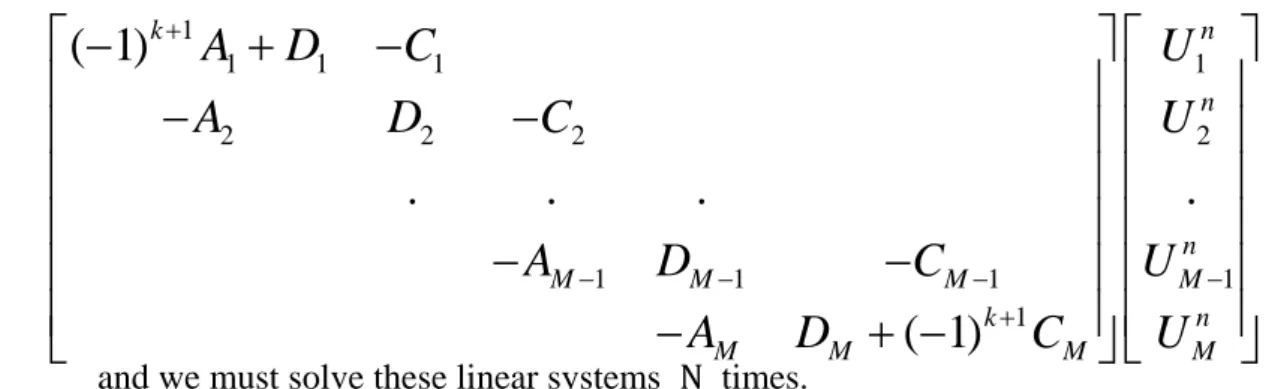
for each k-th Fourier coefficient. Then we could produce the following matrices, 1 1 1 1 1 1 2 2 2 2 1 1 1 1 1 1

( 1)

.

.

.

.

( 1)

k n n n M M M M k n M M M M

A

B

C

U

A

B

C

U

A

B

C

U

A

B

C

U

       







 





 





 





 





 





 





_{ }

 





 



19

=

and we must solve these linear systems N times.

The Step 3 is equal to solve the unknowns in each column of the linear systems as follows,

Figure 5: The order of n here we follow the FFT in MATLAB.

Step 4: We perform inverse fast Fourier transform (IFFT) in θ, After solving the matrices, we do IFFT in each row on our grids. The Step 4 is equal to do IFFT in θ as follows：

Figure 6 1 1 1 1 1 2 2 2 2 1 1 1 1 1

( 1)

.

.

.

.

( 1)

k n n n M M M M k n M M M M

A

D

C

U

A

D

C

U

A

D

C

U

A

D

C

U

     









 





_

_

 





 





 





 









 





_

_{ }

 





 



20

According to the procedure, i.e. Step 1=>Step 2=>Step 3=>Step 4, we could complete the numerical solution at one time step and we can derive the numerical solution at any time by keeping performing the procedure recursively.

3.1.3 Solvers with the Symmetric Discretization

According to [6], we have the formula of the heat equation on a spherical surface domain in spherical coordinates as

ut = ∆su ∆su = ∇s2u = 1 r2 1 sinϕ ∂ ∂ϕ(sinϕ ∂u ∂ϕ) + 1 sin2 _ϕ ∂2_u ∂θ2 (22) Here r is a constant R. We also can derive the surface Laplacian term of (22) and the settings of the grids as Section 3.1.2 says.

Step 1: Similar to Section 3.1.2 Step 1.

Step 2: Similar to Section 3.1.2 Step 2 and substitute (18) into (22),

∆_su = 1 R2 1 sinϕ ∂ ∂ϕ(sinϕ ∂ uk ϕ N 2−1 k=−N₂ e ikθ ∂ϕ ) + 1 sin2 _ϕ ∂2 _u k ϕ N 2−1 k=−N₂ e ikθ ∂θ2 = 1 R2 1_sinϕ ∂ ∂ϕ(sinϕ ∂u_k ϕ eikθ ∂ϕ N 2−1 k=−N₂ ) + 1 sin2 _ϕ ∂2_u k ϕ eikθ ∂θ2 N 2−1 k=−N₂ = 1 R2 1_sinϕ ∂ ∂ϕ( sinϕ ∂u_k ϕ ∂ϕ N 2−1 k=−N₂ eikθ_{) +} 1 sin2 _ϕ uk ϕ (−k2)eikθ N 2−1 k=−N₂ = 1 R2 1 sinϕ ∂ ∂ϕ(sinϕ ∂u_k ϕ ∂ϕ ) − k2 sin2 _ϕ uk ϕ N 2−1 k=−N₂ eikθ ₍₂₃₎

Substitute the surface Laplacian term of (22) into (17), 1 R2( 1 sinϕ ∂ ∂ϕ(sinϕ ∂un+1 ∂ϕ ) + 1 sin2 _ϕ ∂2_un+1 ∂θ2 ) − 2 ∆tun+1

21 = − 1 R2 1 sinϕ ∂ ∂ϕ sinϕ ∂un ∂ϕ + 1 sin2 _ϕ ∂2_un ∂θ2 − 2 ∆tun (24) Substitute (18) into (24), and from (23) we can derive

1 R2 1 sinϕ ∂ ∂ϕ(sinϕ ∂u_kn+1 _ϕ ∂ϕ ) − k2 sin2 _ϕ ukn+1 ϕ N 2−1 k=−N₂ eikθ₋ 2 ∆tukn+1 ϕ N 2 −1 k=−N₂ eikθ = − 1 R2 1 sinϕ ∂ ∂ϕ(sinϕ ∂u_kn _ϕ ∂ϕ ) − k2 sin2 _ϕ ukn ϕ N 2−1 k=−N₂ eikθ ₋ 2 ∆tukn ϕ N 2−1 k=−N₂ eikθ => 1 R2 1 sinϕ ∂ ∂ϕ(sinϕ ∂u_kn+1 _ϕ ∂ϕ ) − k2 sin2 _ϕ ukn+1 ϕ − 2 ∆tukn+1 ϕ N 2−1 k=−N₂ eikθ = − 1 R2 1 sinϕ ∂ ∂ϕ(sinϕ ∂u_kn _ϕ ∂ϕ ) − k2 sin2 _ϕ ukn ϕ − 2 ∆tukn ϕ N 2−1 k=−N₂ eikθ Eliminate and N 2−1 k=−N₂ e

ikθ _{from both sides of the equation,}

1 R2( 1 sinϕ ∂ ∂ϕ(sinϕ ∂u_kn+1 _ϕ ∂ϕ ) − k2 sin2 _ϕ ukn+1 ϕ ) − 2 ∆tukn+1 ϕ = − 1 R2( 1 sinϕ ∂ ∂ϕ(sinϕ ∂u_kn ϕ ∂ϕ ) − k2 sin2 _ϕ ukn ϕ ) − 2 ∆tukn ϕ

After multiplying by R2 to both sides of the equation and equaling the Fourier coefficients, u_k ϕ satisfies 1 sinϕ ∂ ∂ϕ(sinϕ ∂u_kn+1 _ϕ ∂ϕ ) − k2 sin2 _ϕ ukn+1 ϕ − 2R2 ∆t ukn+1 ϕ = − 1 sinϕ ∂ ∂ϕ sinϕ ∂u_kn ϕ ∂ϕ + k2 sin2 _ϕ ukn ϕ − 2R2 ∆t ukn ϕ

The Step 2 is equal to do FFT for θ as Figure 4. Step 3: We use the symmetric discretization for ϕ, i.e.

∂

∂ϕ(sin(ϕi) ∂U_i

∂ϕ) ≈ sinϕ

i+12(Ui+1 − Ui) − sinϕi−12(Ui− Ui−1)

22 For each Fourier modes k (k = −N

2, − N 2+ 1, … , 0, 1 , … , N 2 − 1.), we set u_kn+1 _{ϕ = U}n+1 _{at time (n + 1)Δt} u_kn _{ϕ = U}n _{at time nΔt}

and solve the following equations. 1 sinϕ_i sinϕ i+12 Ui+1 n+1_{− U} i n+1 _{− sinϕ} i−12 Ui n+1 _{− U} i−1 n+1 ∆ϕ2 − k2 sin2 _ϕ i Ui n+1 ₋2R2 ∆t Uin+1 = − 1 sinϕ_i sinϕ i+12(Ui+1 n _{− U} i n_{) − sinϕ} i−12(Ui n _{− U} i−1 n ₎ ∆ϕ2 + k2 sin2 _ϕ i Ui n ₋2R2 ∆t Uin for i = 1 , … , M.

Both sides of the equations were multiplied by ∆ϕ2sin ϕ_i and rearrange them, sinϕ i−1₂Ui−1 n+1_{+ −sinϕ} i−1₂− sinϕi+1₂− k2_∆ϕ2 sin ϕ_i − 2R2_∆ϕ2_{sin ϕ} i ∆t Uin+1+ sinϕ_i+1 2Ui+1 n+1 = −sinϕ i−1₂Ui−1 n _{+ sinϕ} i−1₂+ sinϕi+1₂+ k2_∆ϕ2 sin ϕ_i − 2R2_∆ϕ2_{sin ϕ} i ∆t Uin− sinϕ_i+1 2Ui+1 n ₍₂₅₎

Therefore, we could set that

A_i = sinϕ

i−12

B_i = −sinϕ

i−12− sinϕi+12 −

k2_∆ϕ2 sin ϕ_i − 2R2_∆ϕ2_{sin ϕ} i ∆t C_i = sinϕ i+12 Di = −Bi− 4R2_∆ϕ2_{sin ϕ} i ∆t for i = 1 , … , M.

Because the coefficient of U₀ is sinϕ1

2= 0 and the coefficient of UM+1 is

sinϕ_M+1

2 = 0, we have A1 = 0 and CM = 0. Therefore, we do not need symmetric

23

=

Because A_i+1 = sinϕ_i+1

2 = Ci, for i = 1, … , M − 1 , the matrices will become

symmetric matrices and lead to less computations. It reduces above matrices to be

=

And these linear systems need to be solved N times by the Thomas algorithm here. The Step 3 is equal to solve the unknowns in the linear systems in each Fourier mode as Figure 5.

Step 4: Similar to Section 3.1.2 Step 4.

According to the procedure, i.e. Step 1=>Step 2=>Step 3=>Step 4, we could complete the

































































        1 1 1 1 2 1 1 1 1 1 2 2 2 1 1

.

.

.

.

n M n M n n M M M M M

U

U

U

U

B

A

C

B

A

C

B

A

C

B













































































    n M n M n n M M M M M

U

U

U

U

D

A

C

D

A

C

D

A

C

D

1 2 1 1 1 1 2 2 2 1 1

.

.

.

.

































































         1 1 1 1 2 1 1 1 1 1 2 2 2 1 1 1

.

.

.

.

n M n M n n M M M M M

U

U

U

U

B

C

C

B

C

C

B

C

C

B













































































     n M n M n n M M M M M

U

U

U

U

D

C

C

D

C

C

D

C

C

D

1 2 1 1 1 1 2 2 2 1 1 1

.

.

.

.

24

numerical solution at one time step and we can derive the numerical solution at any time by keeping performing the procedure recursively.

3.2 Numerical Results

We provide the exact solution

u = e−2 tR2 _{x + y + z = e}−2 t_R2 _{Rsin ϕ cos θ + Rsin ϕ sin θ + Rcos ϕ (26)}

for the equations 14 and (22), and R is a constant. Given the initial condition as follows,

u0 = Rsin ϕ cos θ + Rsin ϕ sin θ + Rcos⁡(ϕ)

Because we administer semi-implicit second-order Crank-Nicolson method in spatiotemporal term, we could choose the bigger ∆t. It leads to spending less time to get our numerical solution. According to CFL condition, the stability of the Crank-Nicolson method in the equations (14) and (22) needs to satisfy the property

∆t = O(∆x) In our programming, we could pick out

∆t = 1 2π∆x =

1 N.

It leads to faster computation. In next two Section 3.2.1 and Section 3.2.2, we derive the numerical solution at T = 1 and set ∆t = _N1. Here provide the exact solution at T = 1 for (14) and (22) as follows,

u = e−2 1R2_{(Rsin ϕ cos θ + Rsin ϕ sin θ + Rcos⁡(ϕ))}

3.2.1 Results of Solvers with the Central Difference Method

We solved the heat equation (14) u_t = ∆_su on a spherical surface domain by the numerical methods that are FFT, second-order central difference method, Crank-Nicolson method and Thomas algorithm. In Table 1, solve (14) numerically

25

with R = 1 at T = 1 and check them by the exact solution

u = e−2 _{sin ϕ cos θ + sin ϕ sin θ + cos ϕ (27)}

Table 1: The numerical results are second-order accuracy.

In Table 2, solve (14) numerically with R = 5 at T = 1 and check them by the exact solution

u = e− 252 5sin ϕ cos θ + 5sin ϕ sin θ + 5 cos ϕ (28)

Table 2: The numerical results are second-order accuracy.

3.2.2 Results of Solvers with the Symmetric Discretization

We solved the heat equation (22) u_t = ∆_su on a spherical surface domain by numerical methods that are FFT, symmetric discretization, Crank-Nicolson method,

𝐌 × 𝐍 𝐋_∞nrom RATIO ORDER

8 × 16 0.0058 0 0

16 × 32 0.0014 4.1429 2.0506

32 × 64 3.5098e-004 3.9888 1.9960

64 × 128 8.7537e-005 4.0095 2.0034 128 × 256 2.1885e-005 3.9999 2.0000

𝐌 × 𝐍 𝐋_∞nrom RATIO ORDER

8 × 16 0.0050 0 0

16 × 32 0.0011 4.5455 2.1844

32 × 64 2.7313e-004 4.0274 2.0098

64 × 128 6.8221e-005 4.0036 2.0013 128 × 256 1.7053e-005 4.0005 2.0002

26 and Thomas algorithm.

In Table 3, solve (22) numerically with R = 1 at T = 1 and check them by the exact solution (27).

Table 3: The numerical results are second-order accuracy.

In Table 4, solve (22) numerically with R = 5 at T = 1 and check them by the exact solution (28).

Table 4: The numerical results are second-order accuracy.

3.3 Mass Conservation

We developed an interest in keeping a lookout for the variation of the total mass in our numerical solvers due to

d dt u ∂Ω dxdydz = d dt u ∂𝐗 ∂ϕ× ∂𝐗 ∂θ π 0 dϕdθ 2π 0 = 0 (29)

M × N 𝐋_∞nrom RATIO ORDER

8 × 16 0.0090 0 0

16 × 32 0.0022 4.0909 2.0324

32 × 64 5.4423e-004 4.0424 2.0152

64 × 128 1.3612e-004 3.9982 1.9993 128 × 256 3.4027e-005 4.0004 2.0001

𝐌 × 𝐍 𝐋_∞nrom RATIO ORDER

8 × 16 0.0066 0 0

16 × 32 0.0015 4.4000 2.1375

32 × 64 3.7037e-004 4.0500 2.0179

64 × 128 9.2165e-005 4.0186 2.0067 128 × 256 2.2994e-005 4.0082 2.0030

27

∂Ω: spherical surface

x = Rsinϕcosθ, y = Rsinϕsinθ, z = Rcosϕ

𝐗 R, ϕ, θ = x , y , z = Rsinϕcosθ , Rsinϕsinθ , Rcosϕ 𝐗_i,j ≈ 𝐗 ϕ_i, θ_j ∂𝐗 ∂ϕ× ∂𝐗 ∂θ = 𝒾 𝒿 𝓀 ∂x ∂ϕ ∂y ∂ϕ ∂z ∂ϕ ∂x ∂θ ∂y ∂θ ∂z ∂θ

= Rcosϕcosθ𝒾 Rcosϕsinθ −Rsinϕ𝒿 𝓀 −Rsinϕsinθ Rsinϕcosθ 0

= R2_sin2_{ϕcosθ, R}2_sin2_{ϕsinθ, R}2_{sinϕcosϕ cos}2_{θ+ sin}2_θ

= R2_sin2_{ϕcosθ, R}2_sin2_{ϕsinθ, R}2_sinϕcosϕ

∂𝐗 ∂ϕ×

∂𝐗

∂θ = R4sin4ϕ cos2θ+ sin2θ + R4sin2ϕcos2ϕ

1 2

= R4_sin4_{ϕ + R}4_sin2_ϕcos2_{ϕ 2}1 _{= R}4_sin2_{ϕ sin}2_{ϕ + cos}2_ϕ 12

= R2 _sinϕ

Choose specific four cases in our paper to observe the total mass of them which changes with time. Because of immovability of our spherical surface domain, the total mass is equal to

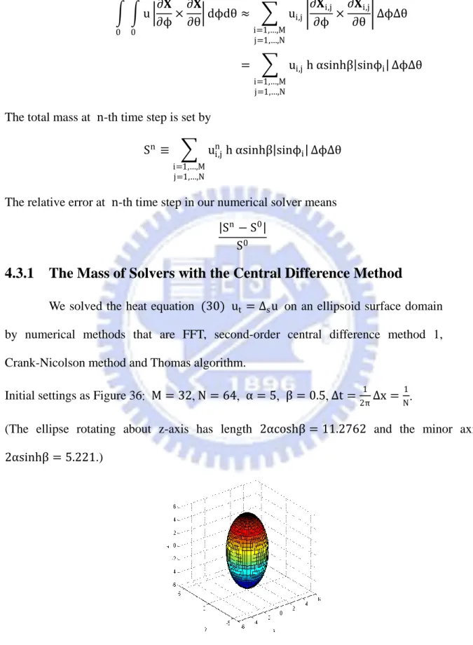
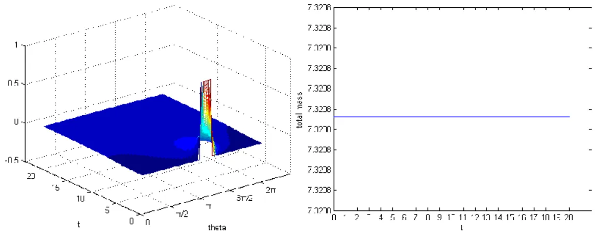
u ∂𝐗 ∂ϕ× ∂𝐗 ∂θ π 0 dϕdθ 2π 0 ≈ ui,j ∂𝐗_i,j ∂ϕ × ∂𝐗_i,j ∂θ i=1,…,M j=1,…,N ΔϕΔθ = ui,jR2 sinϕi i=1,…,M j=1,…,N ΔϕΔθ

The total mass at n-th time step is set by Sn _{≡ u} i,j n_R2 _sinϕ i i=1,…,M j=1,…,N ΔϕΔθ

The relative error at n-th time step in our numerical solver means Sn_{− S}0

S0

3.3.1 The Mass of Solvers with the Central Difference Method

28

Figure 7: The domain is a spherical surface with R = 5. Case 1: Pizza-like initial condition as follows,

u(1:0.5*M,0.5*N:0.5*N+5)=1; others are set to be zero.

Figure 8: Initial value u; T = 0; Total mass = 14.7321.

Figure 9: Left, T = 0.25, mass = 14.7321, relative error = 1.8087e − 015. Mid-left, T = 0.5, mass = 14.7321, relative error = 7.3552e − 015. Mid-right, T = 0.75, mass = 14.7321, relative error = 9.8873e − 015.

29

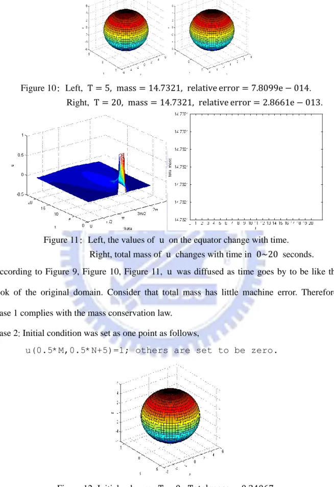
Figure 10: Left, T = 5, mass = 14.7321, relative error = 7.8099e − 014. Right, T = 20, mass = 14.7321, relative error = 2.8661e − 013.

Figure 11: Left, the values of u on the equator change with time. Right, total mass of u changes with time in 0~20 seconds.

According to Figure 9, Figure 10, Figure 11, u was diffused as time goes by to be like the look of the original domain. Consider that total mass has little machine error. Therefore, Case 1 complies with the mass conservation law.

Case 2: Initial condition was set as one point as follows,

u(0.5*M,0.5*N+5)=1; others are set to be zero.

30

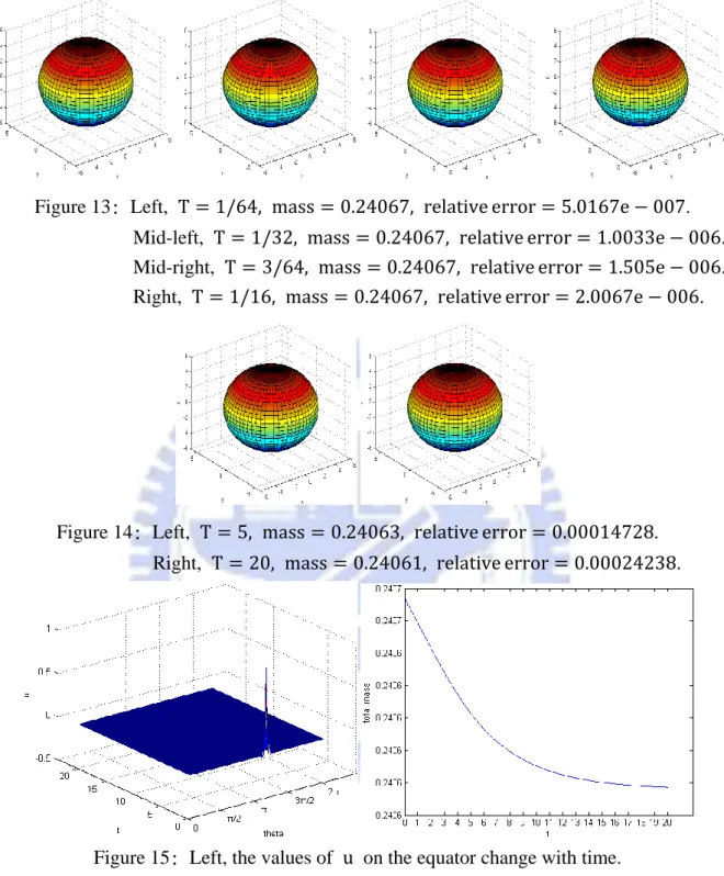
Figure 13: Left, T = 1/64, mass = 0.24067, relative error = 5.0167e − 007. Mid-left, T = 1/32, mass = 0.24067, relative error = 1.0033e − 006. Mid-right, T = 3/64, mass = 0.24067, relative error = 1.505e − 006.

Right, T = 1/16, mass = 0.24067, relative error = 2.0067e − 006.

Figure 14: Left, T = 5, mass = 0.24063, relative error = 0.00014728. Right, T = 20, mass = 0.24061, relative error = 0.00024238.

Figure 15: Left, the values of u on the equator change with time. Right, total mass of u changes with time in 0~20 seconds. According to Figure 13, Figure 14, Figure 15, u was diffused as time goes by to be like the look of the original domain. Total mass is getting decreasing a little bit, but it will turn to stable that means mass will not change any more in a long time. Case 2 does not comply with the mass conservation law.

31 Case 3: Chapeau-like initial condition as follows,

u(1:3,1:N)=1; others are set to be zero.

Figure 16: Initial value u; T = 0; Total mass = 6.7665.

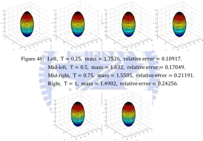
Figure 17: Left, T = 0.25, mass = 6.7665, relative error = 0.00017029. Mid-left, T = 0.5, mass = 6.7686, relative error = 0.00030516. Mid-right, T = 0.75, mass = 6.7693, relative error = 0.00040749. Right, T = 1, mass = 6.7698, relative error = 0.00040878.

Figure 18: Left, T = 5, mass = 6.773, relative error = 0.00095451. Right, T = 20, mass = 6.7743, relative error = 0.001145.

32

Figure 19: Left, the values of u on the equator change with time. Right, total mass of u changes with time in 0~20 seconds. According to Figure 17, Figure 18, Figure 19, u was diffused as time goes by to be like the look of the original domain. Total mass is getting increasing a little bit, but it will turn to stable that means mass will not change any more in a long time. Case 3 does not comply with the mass conservation law.

Case 4: Smooth initial condition as follows, u(m,n)=abs(sin((m-0.5)*π

M))+abs(cos((n-1)* 2π

N)), ∀ m, n.

Figure 20: Initial value u; T = 0; Total mass = 446.6597.

33

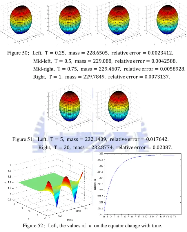
Mid-left, T = 0.5, mass = 446.6566, relative error = 6.9874e − 006. Mid-right, T = 0.75, mass = 446.6553, relative error = 9.8891e − 006.

Right, T = 1, mass = 446.6541, relative error = 1.2529e − 006.

Figure 22: Left, T = 5, mass = 446.6434, relative error = 3.6478e − 005. Right, T = 20, mass = 446.6373, relative error = 5.0161e − 005.

Figure 23: Left, the values of u on the equator change with time. Right, total mass of u changes with time in 0~20 seconds. According to Figure 21, Figure 22, Figure 23, u was diffused as time goes by to be like the look of the original domain. Total mass is getting decreasing a little bit, but it will turn to stable that means mass will not change any more in a long time. Case 4 does not comply with the mass conservation law.

In above Case 1~Case 4, we derive that Case 1 can get the perfect result by mass conservation with some machine error；the others show up a little bit derivation that is less than one percent in our relative error.

3.3.2 The Mass of Solvers with the Symmetric Discretization

34 Case 1: Initial values are the same as Figure 8,

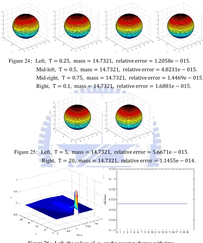
Figure 24: Left, T = 0.25, mass = 14.7321, relative error = 1.2058e − 015. Mid-left, T = 0.5, mass = 14.7321, relative error = 4.8231e − 015. Mid-right, T = 0.75, mass = 14.7321, relative error = 1.4469e − 015.

Right, T = 0.1, mass = 14.7321, relative error = 1.6881e − 015.

Figure 25: Left, T = 5, mass = 14.7321, relative error = 5.6671e − 015. Right, T = 20, mass = 14.7321, relative error = 1.1455e − 014.

Figure 26: Left, the values of u on the equator change with time. Right, total mass of u changes with time in 0~20 seconds. According to Figure 24, Figure 25, Figure 26, u was diffused as time goes by to be like the look of the original domain. Consider that total mass has little machine error. Therefore, Case 1 complies with the mass conservation law.

35 Case 2: Initial values are the same as Figure 12,

Figure 27: Left, T = 1/64, mass = 0.24067, relative error = 6.9197e − 016. Mid-left, T = 1/32, mass = 0.24067, relative error = 8.0729e − 016..

Mid-right, T = 3/64, mass = 0.24067, relative error = 1.1533e − 016. Right, T = 1/16, mass = 0.24067, relative error = 2.3066e − 015.

Figure 28: Left, T = 5, mass = 0.24067, relative error = 5.6511e − 015. Right, T = 20, mass = 0.24067, relative error = 4.9591e − 015.

Figure 29: Left, the values of u on the equator change with time. Right, total mass of u changes with time in 0~20 seconds. According to Figure 27, Figure 28, Figure 29, u was diffused as time goes by to be like the look of the original domain. Consider that total mass has little machine error. Therefore, Case 2 complies with the mass conservation law.

36 Case 3: Initial values are the same as Figure 16,

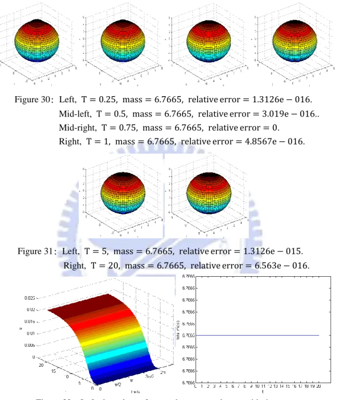
Figure 30: Left, T = 0.25, mass = 6.7665, relative error = 1.3126e − 016. Mid-left, T = 0.5, mass = 6.7665, relative error = 3.019e − 016..

Mid-right, T = 0.75, mass = 6.7665, relative error = 0. Right, T = 1, mass = 6.7665, relative error = 4.8567e − 016.

Figure 31: Left, T = 5, mass = 6.7665, relative error = 1.3126e − 015. Right, T = 20, mass = 6.7665, relative error = 6.563e − 016.

Figure 32: Left, the values of u on the equator change with time. Right, total mass of u changes with time in 0~20 seconds.

According to Figure 30, Figure 31, Figure 32, u was diffused as time goes by to be like the look of the original domain. Consider that total mass has little machine error. Therefore, Case 3 complies with the mass conservation law.

37 Case 4: Initial values are the same as Figure 20,

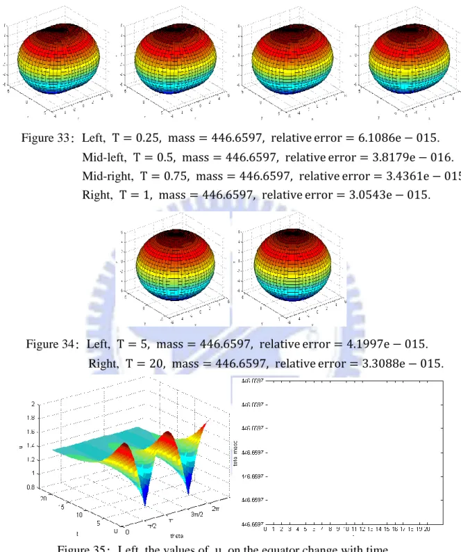
Figure 33: Left, T = 0.25, mass = 446.6597, relative error = 6.1086e − 015. Mid-left, T = 0.5, mass = 446.6597, relative error = 3.8179e − 016.

Mid-right, T = 0.75, mass = 446.6597, relative error = 3.4361e − 015 Right, T = 1, mass = 446.6597, relative error = 3.0543e − 015.

Figure 34: Left, T = 5, mass = 446.6597, relative error = 4.1997e − 015. Right, T = 20, mass = 446.6597, relative error = 3.3088e − 015.

Figure 35: Left, the values of u on the equator change with time. Right, total mass of u changes with time in 0~20 seconds.

According to Figure 33, Figure 34, Figure 35, u was diffused as time goes by to be like the look of the original domain. Consider that total mass has little machine error. Therefore, Case 4 complies with the mass conservation law.

38 law and leave some machine error here.

3.3.3 Comparison between the Central Difference Method and the

Symmetric Discretization in Spherical Coordinates

According to the results in Section 3.3.1 and Section 3.3.2, we could summarize the following table:

𝟑. 𝟑. 𝟏 𝟑. 𝟑. 𝟐 Case1 2.8661e-013 1.1455e-014 Case2 0.00024238 4.9591e-015 Case3 0.001145 6.563e-016 Case4 5.0161e-005 3.3088e-015

Table 5: The relative error in four cases with different numerical methods at T = 20. We are satisfied with the results in the four cases of the solvers in Section 3.3.2 because they comply with the mass conservation law and they only leave indelible and negligible machine error with us. Before discussing farther, introduce that why these four cases are handpicked as follows:

Case 1: The initial values are given from the pole to the equator, and they cross through the dense grids near the poles and the dissipative grids near the equator. This case contains all situations which could average the diversity of geometry.

Case 2: The initial value is given one point. The case could extend to all cases which are composed of some discrete points.

Case 3: The initial value capped the poles which are the densest position in our grids. We could understand how the values in the poles which are usually the singularities in. Case 4: We give the smooth initial values which are different from preceding three cases. Due to the results of above illustrations, we believe that the solvers in Section 3.3.2 will make any initial condition keep the mass conservation law. Table 5 brings us that the symmetric