車間電波傳播模型之建構與量測

全文

(1)國立交通大學電信工程學系碩士論文. 車間電波傳播模型之建構與量測. Modeling and Measurements of Vehicle-to-Vehicle Radio Propagation. 研究生：鍾和穆指導教授：唐震寰博士. 中華民國九十四年七月.

(2) 車間電波傳播模型之建構與量測 Modeling and Measurements of Vehicle-to-Vehicle Radio Propagation. 研究生：鍾和穆. Student : He-Mu Chong. 指導教授：唐震寰. Advisor : Dr. Jenn-Hwan Tarng. 國立交通大學電信工程學系碩士班碩士論文. A Thesis Submitted to Department of Communication College of Engineering National Chiao Tung University in Partial Fulfillment of the Requirements for the Degree of Master of Science in Communication Engineering July 2005 Hsinchu, Taiwan, Republic of China 中華民國九十四年七月. I.

(3) 車間電波傳播模型之建構與量測研究生:鍾和穆. 指導教授:唐震寰博士. 國立交通大學電信工程研究所摘要本論文提供行動車機對行動車機之間的電波傳播模型，與通道特性之量測於 900MHz 以及 1200MHz 。它是由適應環境式模型 (Site-specific Model)和統計模型組合而成，適應環境式模型可計算直接波地面反射波與牆壁的散射波。而散射模型則可用來描述傳播環境中隨機擺放的散射體所造成的散射場。藉由電波場強量測實驗數據與該模型模擬結果之比較，混合模式模型能同時可精確地預估電波的傳播路徑損耗、遮蔽效應、以及小尺度衰弱。. I.

(4) Modeling and Measurements of Vehicle-to-Vehicle Radio Propagation Student: He-Mu Chong. Advisor : Dr. Jenn-Hwan. Tarng,. Department of Communication Engineering National Chiao Tung University. Abstract In this paper, vehicle-to-vehicle radio channels are explored and modeled. A deterministic-statistical (hybrid) spatio-temporal model for vehicle-to-vehicle channels is developed. The model combines a deterministic model with a statistical model. The latter one employs statistical approach to calculate the scattered fields due to randomly positioned scatterers in the first Fresnel zone, which represent the vehicles, trees, lampposts, and motorcycles in the zone. The model is validated by comparing the computed result with the measured averaged path loss, shadowing and small scale fading at 900MHz and 1200MHz. The hybrid model has been proved to be effective and accurate.. II.

(5) 致謝首先，我要對我的指導教授唐震寰老師致上最誠摯的感謝，感謝老師在我碩士兩年的研究生涯中，給于我最細心與凡心的指導與叮嚀，並帶領我一窺無線通訊領域研究的奧妙。其次，對於波散射與傳播實驗室的學長與同學們也要致上我深深的謝意，他們所給予我在知識上和精神上的啟示與鼓勵以及在實驗量測中的協助，對完成本篇論文有莫大的助益。最後，要感謝的是我最親愛的父母親、弟弟以及瑋蕾由於他們給予我的支持與關懷，使我在人生的過程裡得到最細心的呵護與照顧，讓我在成長與求學的過程中能夠有所依靠。僅以此篇論文獻給所有關心我的人。. 鍾和穆國立交通大學，新竹市中華民國九十四年七月. III.

(6) Contents Chapter 1: Introduction……………………………………………………………….1 Chapter 2: Measurement of Path Loss for Vehicle-to-Vehicle Environments…...…...4 2.1 Measurement system and setup……………………………………………......4 2.2 Measurement environments……………………….………………….…….…8 2.2.1 Site A (Open Area without Traffic)……………………………………...8 2.2.2 Site B (open Area with traffic)………………………………..…............9 2.2.2 Site C & Site D (roadway in city)……………………..…………….....11 2.3 Measurement Result………………………………………………………….13 2.3.1 Site A…………………………………………………………………...13 2.3.2 Site B…………………………………………………………………...14 2.3.3 Site C…………………………………………………………………...15 2.3.4 Site D…………………………………………………………………...15 Chapter 3: Characterization of Vehicle-to-Vehicle Path Loss.……………………...17 3.1 Average path loss ………………………….……………………………..…..17 3.2 Shadow fading distribution……….…………………………………….……21 3.3 Small scale fading……………………………………………………………33 Chapter 4: Modeling of Vehicle-to-Vehicle Spatio-Temporal Channels……………43 4.1 Model development……………………………………………………….….43 4.1.1 Hybrid model……………………………………………………….…..43 4.1.2 Site-specific model……………………………………………….…….43 4.1.3 Statistical model………………………………………………………..45 4.2 Validation of Hybrid Model……………………………………………..........46 Chapter 5: Conclusion………………………………………………………………54 Reference…………………………………..………………………………………...55. III.

(7) Table Captions Table 3.1 Dual slope path loss exponents and the standard deviation of the shadow fading for 900MHz and 1200MHz of the four sites……………………….19 Table 3.2 Correlation distances at four sites for 900MHz and 1200MHz……………31 Table 3.3 Measured Ricean factors ( K ) at four sites for 900MHz and 1200MHz......................................................................................................34 Table 4.1 Comparisons between measurement data and computed results of the best-fitting path loss exponents and standard deviation of shadow fading distribution (a) 900 MHz; and (b) 1200 MHz……………………………..51 Table 4.2 Comparisons between measurement data and computed results of the correlation distance. (a) 900 MHz ; and (b) 1200 MHz…………………...52 Table 4.3 Comparisons between measurement data and computed results for the Ricean factors. (a) 900 MHz ; and (b) 1200 MHz…………………………53. IV.

(8) Figure Captions Figure 2.1 Vehicle-to-vehicle field strength measurement system…………………….5 Figure 2.2 The photograph of the transmitter………………………………………….6 Figure 2.3 The photograph of the receiver…………………………………………….6 Figure 2.4 The photograph of the transmitter in outdoor……………………………...7 Figure 2.5 The photograph of the receiver in outdoor…………………………………7 Figure 2.6 The measurement route of site A on the map………………………………8 Figure 2.7 The photograph of the site A……………………………………………….9 Figure 2.8 The measurement route of site B on the map……………………………..10 Figure 2.9 The photograph of the site B……………………………………………...10 Figure 2.10 The measurement route of site C on the map……………………………11 Figure 2.11 The photograph of the site C…………………………………………….12 Figure 2.12 The measurement route of site D on the map…………………………...12 Figure 2.13 The photograph of the site D…………………………………………….13 Figure 2.14 Path loss versus Tx-Rx distance of measured data at site A…………….14 Figure 2.15 Path loss versus Tx-Rx distance of measured data at site B…………….14 Figure 2.16 Path loss versus Tx-Rx distance of measured data at site C…………….15 Figure 2.16 Path loss versus Tx-Rx distance of measured data at site D…………….16 Figure 3.1 Measured averaged path loss versus Tx-Rx distance at site A compared with the computed path loss using the dual slope path loss model………19 Figure 3.2 Measured averaged path loss versus Tx-Rx distance at site B compared with the computed path loss using the dual slope path loss model………20 Figure 3.3 Measured averaged path loss versus Tx-Rx distance at site C compared with the computed path loss using the dual slope path loss model………20 Figure 3.4 Measured averaged path loss versus Tx-Rx distance at site D compared with the computed path loss using the dual slope path loss model………21 Figure 3.5 The measured path loss variation versus T-R separation at site A for 900MHz..…………………………………………………………………22 Figure 3.6 Probability density histogram with log-normal fitting curve ( σ = 3.26 dB ) at site A for 900MHz……………………………………………………..22 Figure 3.7 The measured path loss variation versus T-R separation at site A for 1200MHz…………………………………………………………………23 V.

(9) Figure 3.8 Probability density histogram with log-normal fitting curve ( σ = 3.62 dB ) at site A for 1200MHz……………………………………………………23 Figure 3.9 The measured path loss variation versus T-R separation at site B for 900MHz…………………………………………………………………..24 Figure 3.10 Probability density histogram with log-normal fitting curve( σ = 4.03 dB ) at site B for 900MHz……………………………………………………24 Figure 3.11 The measured path loss variation versus T-R separation at site B for 1200MHz………………………………………………………………..25 Figure 3.12 Probability density histogram with log-normal fitting curve( σ = 5.29 dB ) at site B for 1200MHz…………………………………………………..25 Figure 3.13 The measured path loss variation versus T-R separation at site C for 900MHz………………………................................................................26 Figure 3.14 Probability density histogram of the measured with log-normal fitting curve ( σ = 4.74 dB ) at site C for 900MHz…………………………….26 Figure 3.15 The measured path loss variation versus T-R separation at site C for 1200MHz………………………………………………………………. 27 Figure 3.16 Probability density histogram with log-normal fitting curve( σ = 5.93 dB ) at site C for 1200MHz…………………………………………………..27 Figure 3.17 The measured path loss variation versus T-R separation at site D for 900MHz…………………………………………………………………28 Figure 3.18 Probability density histogram with log-normal fitting curve( σ = 5.57 dB ) at site D for 900MHz……………………………………………………28 Figure 3.19 The measured path loss variation versus T-R separation at site D for 1200MHz………………………………………………………………..29 Figure 3.20 Probability density histogram with log-normal fitting curve( σ = 4.18 dB ) at site D for 1200MHz…………………………………………………..29 Figure 3.21 Autocorrelation function versus distance due to the shadow fading at site A…………………………………………………………………….31 Figure 3.22 Autocorrelation function versus distance due to the shadow fading at site B…………………………………………………………………….32 Figure 3.23 Autocorrelation function versus distance due to the shadow fading at site C…………………………………………………………………….32 Figure 3.24 Autocorrelation function versus distance due to the shadow fading at site D…………………………………………………………………….33. VI.

(10) Figure 3.25 The small scale fading variation versus T-R separation distance at site A for 900MHz……………………………………………………………..35 Figure 3.26 Cumulative distribution of small scale fading with Ricean fitting curve ( K=13 ) at site A for 900MHz………………………………………….35 Figure 3.27 The small scale fading variation versus T-R separation distance at site A for 1200MHz……………………………………………………………36 Figure 3.28 Cumulative distribution of small scale fading with Ricean fitting curve ( K=12.5 ) at site A for 1200MHz………………………………………36 Figure 3.29 The small scale fading variation versus T-R separation distance at site B for 900MHz..……………………………………………………………37 Figure 3.30 Cumulative distribution of small scale fading with Ricean fitting curve ( K=6 ) at site B for 900MHz…………………………………………...37 Figure 3.31 The small scale fading variation versus T-R separation distance at site B for 1200MHz……………………………………………………………38 Figure 3.32 Cumulative distribution of small scale fading with Ricean fitting curve ( K=5.8 ) at site B for 1200MHz………………………………………..38 Figure 3.33 The small scale fading variation versus T-R separation distance at site C for 900MHz……………………………………………………………..39 Figure 3.34 Cumulative distribution of small scale fading with Ricean fitting curve ( K=3) on site C at 900MHz…………………………………………….39 Figure 3.35 The small scale fading variation versus T-R separation distance at site C for 1200MHz……………………………………………………………40 Figure 3.36 Cumulative distribution of small scale fading with Ricean fitting curve ( K=2) on site C at 1200MHz…………………………………………...40 Figure 3.37 The small scale fading variation versus T-R separation distance at site D for 900MHz……………………………………………………………..41 Figure 3.38 Cumulative distribution of small scale fading with Ricean fitting curve ( K=2.7) on site D at 900MHz…………………………………………..41 Figure 3.39 The small scale fading variation versus T-R separation distance at site D for 1200MHz……………………………………………………………42 Figure 3.40 Cumulative distribution of small scale fading with Ricean fitting curve ( K=2.5) on site D at 1200MHz…………………………………………42 Figure 4.1 The path geometry on the horizontal plane……………………………….45. VII.

(11) Figure 4.2 Received power versus Tx-Rx distance at site A for 900MHz (a) Measured data; and (b) Computed results…………………………….47 Figure 4.3 Received power versus Tx-Rx distance at site B for 900MHz (a) Measured data ; and (b) Computed results……………………………47 Figure 4.4 Received power versus Tx-Rx distance at site C for 900MHz (a) Measured data; and (b) Computed results…………………………….48 Figure 4.5 Received power versus Tx-Rx distance at site C for 900MHz (a) Measured data ; and (b) Computed results……………………………48 Figure 4.6 Cumulative distribution of small scale fading with Ricean fitting curve at site A for 900MHz. (a) Measured data with Ricean factor, K=13 (b) Computed results with Ricean factor , K=12.3……………………….49 Figure 4.7 Cumulative distribution of small scale fading with Ricean fitting curve at site B for 900MHz. (a) Measured data with Ricean factor, K=6 (b) Computed results with Ricean factor, K=6.7…………………………49 Figure 4.8 Cumulative distribution of small scale fading with Ricean fitting curve at site C for 900MHz. (a) Measured data with Ricean factor, K=3 (b) Computed results with Ricean factor, K=2.4…………………………50 Figure 4.9 Cumulative distribution of small scale fading with Ricean fitting curve at site D for 900MHz. (a) Measured data with Ricean factor, K=2.7 (b) Computed results with Ricean factor, K=2…………………………...50. VIII.

(12) Chapter 1 Introduction. In recent years, mobile ad-hoc networks (MANETs) have received much attention due to their potential applications and proliferation of mobile devices, [1, 2]. Specifically, MANETs mean wireless multi-hop networks formed by a set of mobile nodes without relying on a preexisting infrastructure. Although they are infrastructureless and has many benefits such as self-configuration and ease of deployment, their flexibility and convenience come at a price. The networks still inherit the traditional problems of wireless communications, such as bandwidth optimization, power control, and transmission quality enhancement. In addition, their mobility, multihop nature and the lack of infrastructure create a number of new complexities and design constraints, which include dynamically changing network topologies, network robustness and reliability, hidden-terminal and exposed-terminal problems, variation in link and node capabilities, energy constrained operation and network security. Many of them are due to the time-varying radio channel characteristics since every node, including the source and the target, in the networks is in motion. In addition, low transmitting and receiving antenna heights lead to severe blockage effect, which may be different from that of macrocellular and microcelluar radio systems with the base station antenna height being much larger than that of the mobile station. A profound knowledge of the radio channel characteristics is a prerequisite for the development of efficient wireless transmission systems. To our knowledge, only 1.

(13) few literatures explore vehicle-to-vehicle radio channel characteristics and models. In [3]~[4], the authors present a “double ring” model to simulate the mobile-to-mobile local scattering environment and use it to develop a sum-of-sinusoids based method for simulating small scale fading channels. In [5], analytical expressions of the time-autocorrelation function and the Doppler spectrum in a mobile radio channel are derived in the presence of three-dimensional (3-D) multipath scattering. In [6], fading statistical properties, such as the level-crossing rate and fade duration of the envelope, of mobile-to-mobile land communication channels have been investigated. In [7], the paper present results from vehicle to vehicle RF propagation measurements centered at 900 MHz. The authors focus on determining delay spread and path loss exponents measured by vector network analyzer. In this paper, vehicle-to-vehicle radio channels are explored and modeled. A deterministic-statistical (hybrid) spatio-temporal model for vehicle-to-vehicle channels is developed. The model combines a deterministic model with a statistical model. The former model, a site-specific model, considers the direct wave, ground-reflected waves and the waves reflected from the walls along streets. The latter one employs statistical approach to calculate the scattered fields due to randomly positioned scatterers in the first Fresnel zone, which represent the vehicles, trees, lampposts, and motorcycles in the zone. The model is validated by comparing the computed result with the measured averaged path loss, shadowing and small scale fading at frequencies 900MHz and 1200MHz. The hybrid model has been proved to be effective and accurate. This report is organized as follows. In Chapter 2, the measurement system and measurement environments are described. In Chapter 3, channel parameters such as path loss exponents, the correlation distance, standard deviation of shadowing and the Ricean factor of the vehicle-to-vehicle channels are evaluated and analyzed using the 2.

(14) measured data. The hybrid spatio-temporal model is presented in Chapter 4. Validation of the model is also given. In Chapter 5, the conclusion is presented.. 3.

(15) Chapter 2 Measurement. of. Path. Loss. for. Vehicle-to-Vehicle Environments Narrow-band (CW) signal strength measurements were made at 900 MHz and 1200 MHz in Hsin-Chu city, Taiwan. We choose four measurement sites which include open area without traffic, highway 68 (open area with traffic), Dong-Da road and Kuang-Fu road to discussing the vehicle-to-vehicle channel characteristics in different propagation environments. Resulting data were used for the analyses of fading and propagation loss, as reported herein.. 2.1 Measurement system and setup CW measurements were conducted so as to enable the fast sampling required for the study of fading dynamics on the channels of interest. A schematic diagram of the measurement system is shown in Fig. 2.1. Narrow-band（CW）signal measurements were taken at 900MHz and 1200MHz. A 10-dBm CW signal was transmitted by a half-wavelength dipole antenna at a height 1.5 m above the ground. A GPS module was used to position the location of the transmitter, which is recorded by a notebook. The receiving antenna is a half-wavelength dipole antenna at a height 2 m above the ground. The receiver (Advantest R3261A) can instantaneously measure the signal strength between -10 to -85 dBm over a 300kHz interval. The received data was acquired automatically by a notebook with a GPIB（General Purpose Instrument Bus） card. A GPS module was also used at the receiver to position the location of the 4.

(16) transmitter. The photographs of the transmitter and receiver are shown in Figure 2.2 and Figure 2.3. During the measurement, two vehicles were carrying the transmitter and receiver systems separately and moving along the roadway. The transmitting antenna height and the receiving antenna height are 1.5 m and 2 m, respectively. Both the transmitting and receiving antennas are vertically polarized. As the vehicle moved, the T-R distance versus the received power is recorded.. Figure 2.1 Vehicle-to-vehicle field strength measurement system. 5.

(17) Figure 2.2 The photograph of the transmitter. Figure 2.3 The photograph of the receiver. 6.

(18) Figure 2.4 The photograph of the transmitter in outdoor. Figure 2.5 The photograph of the receiver in outdoor. 7.

(19) 2.2 Measurement Environments 2.2.1 Site A (open area without traffic) The measured route is a 1-km long straight way in the north of the Hsin-Chu city, which planted the shade tree on both sides, and the others are the spacious place. The transmitting antenna and the receiving antenna were put on the roof of the car A and car B, the height of the antenna is 2 meters and 1.5 meters respectively. Figure 2.6 and Figure 2.7 illustrate the sketch map and the photograph of the measured route respectively. In order to fully understand the time-varying property, we have done the quantity 6 times to examine again in the same place.. Figure 2.6 The measurement route of site A on the map. 8.

(20) Figure 2.7 The photograph of the site A. 2.2.2 Site B (open area with traffic) The measurement was done on the highway 68 to represent the open area with traffic. The site B is the overpass way, there are few buildings on both sides. There are a lot of cars on site B, which may result in scattering effects. Figure 2.8 and Figure 2.9 illustrate the sketch map and the photograph of the measured route respectively.. 9.

(21) Figure 2.8 The measurement route of site B on the map. Figure 2.9 The photograph of the site B 10.

(22) 2.2.3. Site C & Site D (roadway in city). The measurements were done on roadways in City, which are Dong-Da road (site C) and Kuang-Fu road (site D) in Hsin-Chu City. Usually, the volume of traffic is quite large on both roadways, which may result in scattering effects and sometimes obstructed the direct path. There are a lot of buildings on both sides. The different between site C and site D is that the road width of site C is greater than site D. Figure 2.10 ~Figure 2.13 illustrate the sketch map and the photograph of the measured routes respectively.. Figure 2.10 The measurement route of site C on the map. 11.

(23) Figure 2.11 The photograph of the site C. Figure 2.12 The measurement route of site D on the map 12.

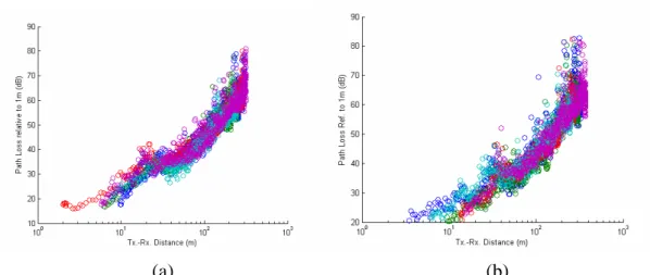
(24) Figure 2.13 The photograph of the site D. 2.3 Measurement result 2.3.1 Site A Figure 2.14a and Figure 2.14b show the measured path loss versus Tx.-Rx distance at frequency 900 MHz and 1200 MHz respectively. It can be observe obviously that the path loss increase with Tx.-Rx. separation distance. Because of fewer obvious reflectors or cars, the field strength varies slightly comparing with the other sites.. 13.

(25) (a) (b) Figure 2.14 Path loss versus Tx-Rx distance of measured data at site A (a) 900MHz ; and (b) 1200MHz. 2.3.2 Site B The site B is the overpass way, there are few buildings on both sides. Because of the cars which move along with the transmitter or receiver, it may induce deep fading due to destructive or constructive interference. Figure 2.15a and Figure 2.15b show the measured path loss versus T-R separation at frequency 900 MHz and 1200 MHz respectively.. (a) (b) Figure 2.15 Path loss versus Tx-Rx distance of measured data at site B (a) 900MHz ; and (b) 1200MHz. 14.

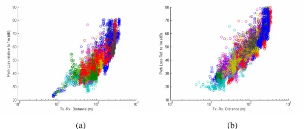
(26) 2.3.3 Site C Site C is a general roadway with buildings on both sides and a lot of cars near the transmitter and receiver. It may produce the serious multipath effect and shadowing effect. It can be observe obviously that the variation of the measured field strength become more serious. Figure 2.16a and Figure 2.16b show the measured path loss versus Tx-Rx distance at 900 MHz and 1200 MHz, respectively.. (a) (b) Figure 2.16 Path loss versus Tx-Rx distance of measured data at site C (a) 900MHz ; and (b) 1200MHz.. 2.3.4 Site D The measured results at site D are similar to the results at site C. Figure 2.17a and Figure 2.17b show the measured path loss versus the Tx-Rx separation at 900 MHz and 1200 MHz, respectively.. 15.

(27) (a). (b). Figure 2.17 Path loss versus Tx-Rx distance of measured data at site D (a) 900MHz ; and (b) 1200MHz. 16.

(28) Chapter 3 Characterization of Vehicle-to-Vehicle Path Loss Narrowband propagation measurements have been conducted in the previous chapter. The narrowband propagation is characterized in terms of averaged path loss, shadowing effect, and small scale fading. With massive measurement results, it is found that (1) the dual slope empirical path loss model is suitable to describe averaged vehicle-to-vehicle path loss; (2) The lognormal distribution basically fits the shadow fading of the received signal well; and (3) The small scale fading still follows a Ricean distribution.. 3.1 Averaged path loss Since both the transmitting and receiving antenna heights are lower than street building heights, which is the same as that of microcellular environments, the dual slope empirical model is adopted to describe the averaged path loss. The model is given by [9] ⎛ d ⎞ PL(d ) = PL(d 0 ) + 10n1 log(d ) + 10(n2 − n1 ) log⎜⎜1 + ⎟⎟ ⎝ db ⎠. (3.1). where n1 and n 2 are unknown parameters and PL(d 0 ) is the path loss in decibels at the reference distance of d 0 = 1m . Again, n1 and n2 are the path loss exponents for the model. d b is the break distance ( d b =100m). These two unknowns can be determined in closed form based on the MMSE criterion 17.

(29) [10], where the variance or mean squared error σ 2 is the quantity to be minimized. For a total of N measurement locations, the mean squared error is. σ2 =. 1 N. N. ∑ (PL i =1. i. − PL(d i )). 2. (3.2). where PLi is the measured path loss in decibels for the i th path loss measurement and PL(d i ) in decibels is evaluated at the T-R separation distance d i in meters for the i th measurement location. σ represent the standard deviation of the shadow fading. Table 3.1 shows the best-fitting results with the dual slope path loss model at four measurement sites at frequency 900MHz and 1200MHz. An important result shown in Table 3.1 is that the path loss exponents for these four sites are all in the ranges of 1.9 ≤ n1 ≤ 2.1 and 4.0 ≤ n 2 ≤ 4.2 . These results indicate that the two-ray or three-ray model may accurately predict the averaged path loss of vehicle-to-vehicle propagation. From the table it can be seen that the rms errors ( σ in decibels) increase when measurement sites become complex; it is greatest on roadways and smallest in the open area without traffic. Figures 3.1, 3.2, 3.3 and 3.4 show measured average path loss versus Tx-Rx distance at sites A, B, C and D, respectively, compared with the computed path loss using the dual slope path loss model.. 18.

(30) Table 3.1 Dual slope path loss exponents and the standard deviation of the shadow fading for 900MHz and 1200MHz of the four sites. Measurement. 900MHz. 1200MHz. sites. n1. n2. σ (dB ). n1. n2. σ (dB ). Site A. 2. 4.1. 3.26. 1.9. 4.1. 3.62. Site B. 1.9. 4.0. 4.03. 1.9. 4.1. 5.29. Site C. 1.9. 4.0. 4.74. 2. 4.0. 5.93. Site D. 2.1. 4.2. 5.57. 2.1. 4.1. 5.04. (a) (b) Figure 3.1 Measured averaged path loss versus Tx-Rx distance at site A compared with the computed path loss using the dual slope path loss model: (a) 900MHz with n1 = 2 and n 2 = 4.1 ; and (b) 1200MHz with n1 = 1.9 and n 2 = 4.1 .. 19.

(31) (a) (b) Figure 3.2 Measured path loss versus Tx-Rx distance at site B compared with the computed path loss using the dual slope path loss model: (a) 900MHz with n1 = 1.9 and n 2 = 4 ; and (b) 1200MHz with n1 = 1.9 and n 2 = 4.1 .. (a) (b) Figure 3.3 Measured path loss versus Tx-Rx distance at site C compared with the computed path loss using the dual slope path loss model: (a) 900MHz with n1 = 1.9 and n 2 = 4 ; and (b) 1200MHz with n1 = 2 and n 2 = 4 .. 20.

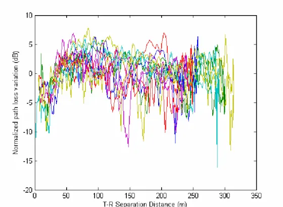
(32) (a) (b) Figure 3.4 Measured path loss versus Tx-Rx distance at site D compared with the computed path loss using the dual slope path loss model: (a) 900MHz with n1 = 2.1 and n 2 = 4.2 ; and (b) 1200MHz with n1 = 2.1 and n 2 = 4.1 .. 3.2 Shadow fading distribution The shadowing contribution to the global attenuation had to be extracted [8]. The small-scale fading is easily discarded by computing local means of the received field using a 10λ sliding window. Figures 3.5 and 3.6 illustrate the measured path loss variation due to shadow fading on a receiver moving away from a transmitter as a function of separation distance and its probability density histogram with log-normal fitting curve at site A for 900MHz. Figure 3.8-3.20 illustrate the same measured results at site B, site C, and site D for 900 MHz and 1200 MHz respectively. .. 21.

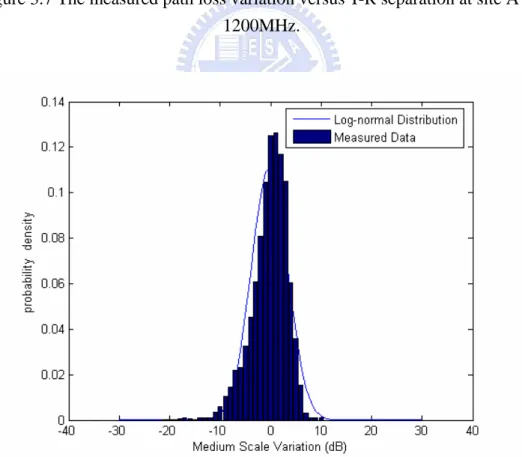
(33) Figure 3.5 The measured path loss variation versus T-R separation at site A for 900MHz.. Figure 3.6 Probability density histogram with log-normal fitting curve ( σ = 3.26 dB ) at site A for 900MHz.. 22.

(34) Figure 3.7 The measured path loss variation versus T-R separation at site A for 1200MHz.. Figure 3.8 Probability density histogram with log-normal fitting curve ( σ = 3.62 dB ) at site A for 1200MHz.. 23.

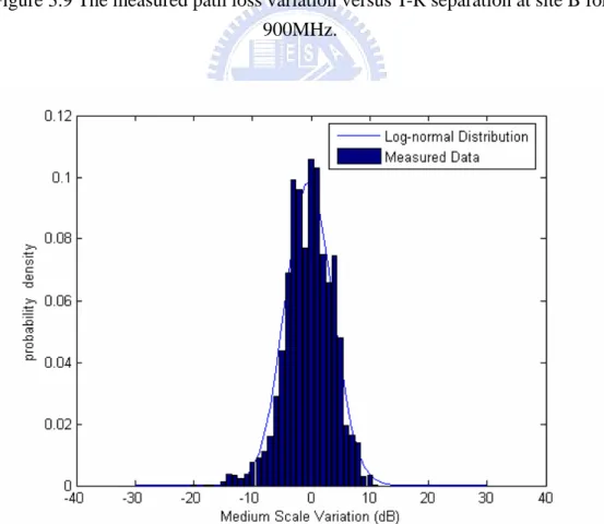
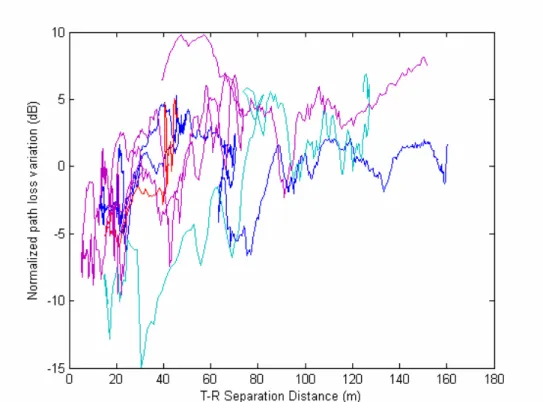
(35) Figure 3.9 The measured path loss variation versus T-R separation at site B for 900MHz.. Figure 3.10 Probability density histogram with log-normal fitting curve ( σ = 4.03 dB ) at site B for 900MHz.. 24.

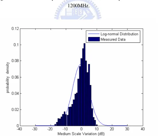
(36) Figure 3.11 The measured path loss variation versus T-R separation at site B for 1200MHz.. Figure 3.12 Probability density histogram with log-normal fitting curve ( σ = 5.29 dB ) at site B for 1200MHz.. 25.

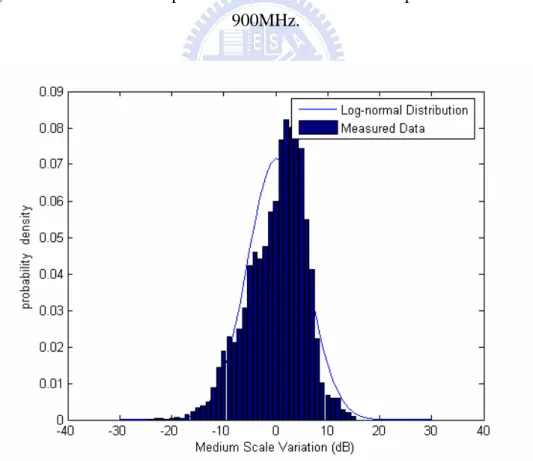
(37) Figure 3.13 The measured path loss variation versus T-R separation at site C for 900MHz.. Figure 3.14 Probability density histogram of the measured with log-normal fitting curve ( σ = 4.74 dB ) at site C for 900MHz.. 26.

(38) Figure 3.15 The measured path loss variation versus T-R separation at site C for 1200MHz.. Figure 3.16 Probability density histogram with log-normal fitting curve ( σ = 5.93 dB ) at site C for 1200MHz.. 27.

(39) Figure 3.17 The measured path loss variation versus T-R separation at site D for 900MHz.. Figure 3.18 Probability density histogram with log-normal fitting curve ( σ = 5.57 dB ) at site D for 900MHz.. 28.

(40) Figure 3.19 The measured path loss variation versus T-R separation at site D for 1200MHz.. Figure 3.20 Probability density histogram with log-normal fitting curve ( σ = 5.04 dB ) at site D for 1200MHz. 29.

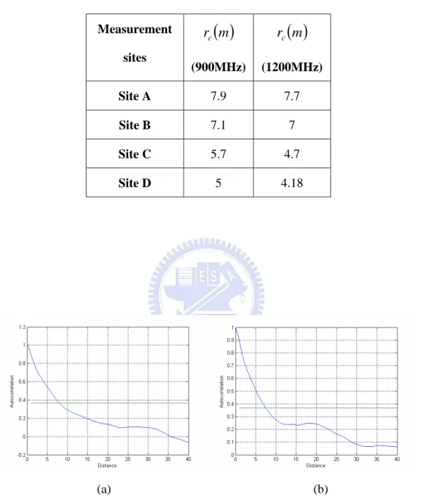
(41) In order to discuss the time-varying property of the propagation channels, we consider the parameter of the shadowing correlation distance. The autocorrelation of the shadow fading process over a range of lags [11] is computed, using Equation (3.3). The lags correspond to a range of distances traveled. n. 1 ~ xi = xi − ∑ xi n i =1 n 1 ~ xi ~ xi − k ∑ n − k i = k +1 ρk = 1 n ~2 ∑ xi n i =1. (3.3). where xi represents the path loss variation of T-R distance, d i . Here, ρ k represents the autocorrelation of k th lag. Measurements of the shadowing autocorrelation process suggest that a simple exponential model of the process is appropriate, characterized by the shadowing correlation distance, rc , the distance taken for the normalized autocorrelation to fall to 1 e of its value. In macrocells, the correlation distance is a few tens or hundreds of meters, and corresponds to the widths of the buildings and other obstructions that are found closest to the mobile. In our research, the correlation distances are below ten meters in mobile-to-mobile channels. It is because both transmitter and receiver are moving simultaneously, which will decrease the correlation distances. Table 3.2 shows the correlation distances at four sites for 900MHz and 1200MHz. From the table it can be seen that the correlation distances decrease when measurement sites become complex and when measurement frequency increase. Figures 3.21, 3.22, 3.23, and 3.24 illustrate the autocorrelation functions of the slow fading or shadowing at four sites for 900MHz and 1200MHz.. 30.

(42) Table 3.2 Correlation distances at four sites for 900MHz and 1200MHz. rc (m ). rc (m ). (900MHz). (1200MHz). Site A. 7.9. 7.7. Site B. 7.1. 7. Site C. 5.7. 4.7. Site D. 5. 4.18. Measurement sites. (a) (b) Figure 3.21 Autocorrelation function versus distance due to the shadow fading at site A (a) Correlation distance, rc = 7.9 m, at 900MHz ; and (b) Correlation distance, rc = 7.7 m, at 1200MHz.. 31.

(43) (a) (b) Figure 3.22 Autocorrelation function versus distance due to the shadow fading at site B (a) Correlation distance, rc = 7.1 m, at 900MHz ; and (b) Correlation distance, rc = 7.0 m, at 1200MHz.. (a) (b) Figure 3.23 Autocorrelation function versus distance due to the shadow fading at site C (a) Correlation distance, rc = 5.7 m, at 900MHz ; and (b) Correlation distance, rc = 4.7 m, at 1200MHz.. 32.

(44) (a) (b) Figure 3.24 Autocorrelation function versus distance due to the shadow fading at site D (a) Correlation distance, rc = 5.0 m, at 900MHz ; and (b) Correlation distance, rc = 3.7 m, at 1200MHz.. 3.3 Small scale fading Small scale fading contribution to the fading in short distance, which is relative to correlation distance, had to be extracted. In a mobile-to-mobile channel, small scale fading is due to the small path length differences between rays coming from scatterers in the neighborhood of the mobile. These differences, on the order of a few wavelengths, lead to significant phase differences. Here, the amplitude statistics of received signal on each measured sites has been fitted by using a Ricean distribution [12]. Figures 3.25 and 3.26 illustrate the measured signal variation due to small scale fading on a receiver moving away from a transmitter as a function of separation distance and its cumulative distribution with Ricean fitting curve at site A for 900MHz. It is found that the Rician distribution yields good fitting result. Figure 3.27-3.40 illustrate the same measured results at site B, site C, and site D for 900 MHz and 1200 MHz respectively. Table 3.3 shows the Ricean factors of four measurement sites at 900MHz and 1200MHz. From the table it can be seen that the Ricean factors ( K ) increase when measurement sites become clear; it is greatest on the open area and smallest on roadways. 33.

(45) Table 3.3 Measured Ricean factors ( K ) at four sites for 900MHz and 1200MHz. Measurement. K. K. (900MHz). (1200MHz). Site A. 13. 12.5. Site B. 6. 5.8. Site C. 3. 2. Site D. 2.7. 2.5. sites. 34.

(46) Figure 3.25 The small scale fading variation versus T-R separation distance at site A for 900MHz. Figure 3.26 Cumulative distribution of small scale fading with Ricean fitting curve ( K=13 ) at site A for 900MHz.. 35.

(47) Figure 3.27 The small scale fading variation versus T-R separation distance at site A for 1200MHz. Figure 3.28 Cumulative distribution of small scale fading with Ricean fitting curve ( K=12.5 ) at site A for 1200MHz.. 36.

(48) Figure 3.29 The small scale fading variation versus T-R separation distance at site B for 900MHz. Figure 3.30 Cumulative distribution of small scale fading with Ricean fitting curve ( K=6 ) at site B for 900MHz.. 37.

(49) Figure 3.31 The small scale fading variation versus T-R separation distance at site B for 1200MHz. Figure 3.32 Cumulative distribution of small scale fading with Ricean fitting curve ( K=5.8 ) at site B for 1200MHz.. 38.

(50) Figure 3.33 The small scale fading variation versus T-R separation distance at site C for 900MHz. Figure 3.34 Cumulative distribution of small scale fading with Ricean fitting curve ( K=3) on site C at 900MHz.. 39.

(51) Figure 3.35 The small scale fading variation versus T-R separation distance at site C for 1200MHz. Figure 3.36 Cumulative distribution of small scale fading with Ricean fitting curve ( K=2) on site C at 1200MHz.. 40.

(52) Figure 3.37 The small scale fading variation versus T-R separation distance at site D for 900MHz. Figure 3.38 Cumulative distribution of small scale fading with Ricean fitting curve ( K=2.7) on site D at 900MHz.. 41.

(53) Figure 3.39 The small scale fading variation versus T-R separation distance at site D for 1200MHz. Figure 3.40 Cumulative distribution of small scale fading with Ricean fitting curve ( K=2.5) on site D at 1200MHz.. 42.

(54) Chapter 4 Modeling of Vehicle-to-Vehicle Spatio-Temporal Channels. The. hybrid. Spatio-Temporal. channel. model. is. developed. to. describe. vehicle-to-vehicle fading channels. The model will be validated by the measurement data described in Chapter 3.. 4.1 The hybrid model The hybrid (deterministic-statistical) model comprises a site-specific propagation model and a statistical model. In the model, the received electric field after the antenna is determined by a superposition of deterministic and randomly scattered fields [13], which is given by Etotal = E dr + E sr. (4.1). v v v v where E dr = ρ * • ∑ E di and E sr = ∑ E si with ρ * being the complex conjugation of i. i. unit polarization vector of the receiving antenna. E dr represents the deterministic ray field E di computed by the site-specific model. E sr represents the summation of each scattered field E si due to randomly positioned scatterers.. 4.1.1 Site-specific model The site-specific model includes multipath propagation in both vertical and horizontal planes. The vertical plane is defined by the transmitter and the receiver positions and is perpendicular to the earth surface, where propagation paths due to direct 43.

(55) wave and ground-reflected wave are considered. The horizontal plane is perpendicular to the vertical plane, where propagation paths due to wall-reflected waves are considered. v The proposed model includes three major propagation modes: (i) a direct-path wave, E D ;. v (ii) a ground-reflected wave, EG ; and (iii) the reflected field from the walls along the v roadway, EW . Summation of these waves determines the receiving field at the observation position and yields. v v v v E dr = E D + EG + EW. (4.2). The ground-reflected wave, is given by. v v EG = E o Gt Gr L f (d ) R g (θ g ). (4.3). And, the wall-reflected wave, is given by. v v EW = Eo Gt Gr L f (d ) Rw (θ w ). (4.4). v. where Eo is the field one meter away from the transmitting antenna. Gt and Gr are the field amplitude patterns of the transmitting and the receiving antennas, respectively. L f (d ) =. e − jkd 4πd. is the free-space propagation factor with an unfolded path length d . Rg (θ g ). is the Fresnel reflection coefficient of ground with an incident angle θ g . R w (θ w ) is the Fresnel reflection coefficient of the walls along the roadway with an incident angle. θw. .. v The direct wave ED can be obtained from Eq.(4.3) by setting R g = 1 .. It is noted that the ground reflected wave will be blocked by the neighboring cars around the transmitter and the receiver and is neglected. It is assumed that this situation will always happen for heavy traffic situation on the roadway in city.. 4.1.2. Statistical model 44.

(56) In the evaluation of the scattered field, the Geometrically Based Single Bounce Elliptical Model (GBSBEM) [14] has been employed to determine the sampled positions of scatterers as shown in Figure 4.1.. Buildings v EW 1. Mobile B. v ED d2. Mobile A. d1. W. v E si. scatterer. e l zon e n s t Fre s r i F v EW 2. Buildings Figure 4.1 The path geometry on the horizontal plane.. v E sr is given as the summation of the scattered field due to each scatterer: [ NV ] v v E sr = ∑ E si. (4.5). i =1. Here, N and V are the scatterer number density (per unit area) and the area of the Fresnel zone, respectively. [ N V ] represents the maximum integer number of N V . And, the scatterers are assumed to distribute uniformly in the region of the ellipse, the first v Fresnel zone. The i th random scattered field E si is given by v v E si = αE 0 Gt G r L f (d1 ) L f (d 2 ). (4.6). where α is the scattering attenuation factor, which is assumed to be uniformly distributed in the region from 0 to 1. 45.

(57) From the definition of the Fresenl zone, the major axis half length a m and the minor axis half length bm of the ellipse are given by. am =. λ 4. +. d0 , 2. 1 ⎛λ ⎞ 2 bm = ⎜ + d0 ⎟ − d0 , 2 ⎝2 ⎠ 2. (4.7). 4.2 Validation of the hybrid model The model is verified by the measured data at the four sites measured at 900 MHz and 1200 MHz. Figures 4.2, 4.3, 4.4 and 4.5 illustrate the 900 MHz measured data and the computed results of the received power versus T-R distance for site A, site B, site C and site D, respectively. It is found that the hybrid model has reasonable prediction accuracy of the received power at four sites. It also found that N =0.08 at site A, N =0.12 at site B, and N =0.3 at sites C and D may be suitable values. Figures 4.2, 4.3,. 4.4 and 4.5 illustrate the 900 MHz measured data and the computed results of cumulative distribution of small scale fading with Ricean fitting curve for site A, site B, site C, and site D, respectively. It is also found that the hybrid model still has better prediction accuracy of the Ricean factor K . Table 4.1 shows the best-fitting path loss exponents and the standard deviations of shadowing at four sites for measured data and computed results. Table 4.2 shows the correlation distances for measured data and computed results. There is a larger difference between the measured and computed results for open area. It is probably because that the reflected waves from far reflectors are neglected. Table 4.3 shows the Ricean factors for measured data and computed results. From these tables, it can be found that the hybrid model present the good prediction accuracy of the vehicle-to-vehicle channel fading characteristics.. 46.

(58) (a) (b) Figure 4.2 Received power versus Tx-Rx distance at site A for 900MHz (a) Measured data; and (b) Computed results. (a) (b) Figure 4.3 Received power versus Tx-Rx distance at site B for 900MHz (a) Measured data ; and (b) Computed results. 47.

(59) (a) (b) Figure 4.4 Received power versus Tx-Rx distance at site C for 900MHz (a) Measured data ; and (b) Computed results. (a) (b) Figure 4.5 Received power versus Tx-Rx distance at site D for 900MHz (a) Measured data ; and (b) Computed results. 48.

(60) (a) (b) Figure 4.6 Cumulative distribution of small scale fading with Ricean fitting curve at site A for 900MHz. (a) Measured data with Ricean factor, K=13 (b) Computed results with Ricean factor , K=12.3. (a) (b) Figure 4.7 Cumulative distribution of small scale fading with Ricean fitting curve at site B for 900MHz. (a) Measured data with Ricean factor, K=6 (b) Computed results with Ricean factor, K=6.7. 49.

(61) (a) (b) Figure 4.8 Cumulative distribution of small scale fading with Ricean fitting curve at site C for 900MHz. (a) Measured data with Ricean factor, K=3 (b) Computed results with Ricean factor, K=2.4. (a) (b) Figure 4.9 Cumulative distribution of small scale fading with Ricean fitting curve at site D for 900MHz. (a) Measured data with Ricean factor, K=2.7 (b) Computed results with Ricean factor, K=2. 50.

(62) Table 4.1 Comparisons between measurement data and computed results of the best-fitting path loss exponents and standard deviation of shadow fading distribution (a) 900 MHz; and (b) 1200 MHz. Measurement sites. Measured Data. Computed Results. n1. n2. σ (dB ). n1. n2. σ (dB ). Site A. 2. 4.1. 3.26. 2.0. 3.9. 3.42. Site B. 1.9. 4.0. 4.03. 2.0. 3.9. 3.57. Site C. 1.9. 4.0. 4.74. 2.0. 4.0. 4.88. Site D. 2.1. 4.2. 5.57. 2.1. 4.1. 5.02. (a). Measurement sites. Measured Data. Computed Results. n1. n2. σ (dB ). n1. n2. σ (dB ). Site A. 1.9. 4.1. 3.62. 2.0. 4.0. 3.71. Site B. 1.9. 4.1. 5.29. 2.0. 4.0. 3.95. Site C. 2. 4.0. 5.93. 2.0. 4.1. 5.36. Site D. 2.1. 4.1. 5.04. 2.1. 4.2. 5.52. (b). 51.

(63) Table 4.2 Comparisons between measurement data and computed results of the correlation distance. (a) 900 MHz ; and (b) 1200 MHz.. rc (m ). rc (m ). (measured). (computed). Site A. 7.9. 10.2. Site B. 7.1. 9.9. Site C. 5.7. 6.8. Site D. 5. 6.1. Measurement sites. (a). rc (m ). rc (m ). (measured). (computed). Site A. 7.7. 8.7. Site B. 7. 8.3. Site C. 4.7. 5.8. Site D. 3.7. 5.2. Measurement sites. (b). 52.

(64) Table 4.3 Comparisons between measurement data and computed results for the Ricean factors. (a) 900 MHz ; and (b) 1200 MHz. Measurement. K. K. (measured). (computed). Site A. 13. 12.3. Site B. 6. 6.7. Site C. 3. 2.4. Site D. 2.7. 2. sites. (a). Measurement. K. K. (measured). (computed). Site A. 12.5. 11.7. Site B. 5.8. 6.2. Site C. 2. 2.1. Site D. 2.5. 1.8. sites. (b). 53.

(65) Chapter 5 Conclusion This thesis presents the measurement channel characteristics and a hybrid spatio-temporal model for vehicle-to-vehicle radio channels. The CW measurement was performed by using spectrum analyzer with GPS module at four sites at 900MHz and 1200MHz. For large scale path loss, the dual slope path loss model provide good accuracy with the path loss exponents; n1 ≅ 2, n 2 ≅ 4 . The log-normal distribution was preformed to describe the shadowing effect. The standard deviations of the shadowing distribution and the correlation distances at four sites are calculated. It can be observed obviously that as the measurement environment become more complex, the standard deviations increase and the correlation distances decrease. Also, it is found that the correlation distances at higher frequency (1200MHz) are always smaller than lower frequency (900MHz). The Ricean distribution was used to perform the small scale fading in our study. The Ricean factor, K , is spread in the range 2~13, it is greatest at clear site and smallest on the roadway. Also, the Ricean factor, K , at 1200MHz are always smaller than 900MHz. The hybrid model is validated by comparing the computed result with the measured averaged path loss, shadowing and small scale fading at frequencies 900MHz and 1200MHz. The model provides accurate prediction for vehicle-to-vehicle fading channels.. 54.

(66) Reference. [1] Ki-Ho Lee; Dong-Ho Cho; “A multiple access collision avoidance protocol for multicast services in mobile ad hoc networks” Communications Letters, IEEE Vol. 7, Issue 10, Oct. 2003 [2] Bellofiore, S.; Foutz, J.; Govindarajula, R.; Bahceci, I.; Balanis, C.A.; Spanias, A.S.; Capone, J.M.; Duman, T.M.; “Smart antenna system analysis, integration and performance for mobile ad-hoc networks (MANETs)” Selected Areas in Communications, IEEE Journal onVolume 18, Issue 9, Sept. 2000 [3] Chirag S. Patel , Gordon L. Stuber and Thomas G. Pratt, “Simulation of Rayleigh Faded Mobile-to-Mobile Communication Channels” VTC 2003-Fall. 2003 IEEE 58th Volume 1,. 6-9 Oct. 2003 Page(s):163 - 167 Vol.1. [4] Li-Chun Wang and Yun-Huai Cheng, “A statistical mobile-to-mobile Rician fading channel model,” IEEE 2004. [5] Francesco Vatalaro,, and Alessandro Forcella, “Doppler Spectrum in Mobile-to-Mobile Communications in the Presence of Three-Dimensional Multipath Scattering” IEEE, Transactions on vehicular tech. VOL. 46, NO. 1, February 1997 [6] Abdulkader S . Akki,“Statistical Properties of Mobile-to-Mobile Land Communication Channels” Transactions on vehicular tech. VOL. 43, NO. 4. November 1994 [7] John S. Davis, and Jean Paul M.G. Linnartz, “Vehicle to Vehicle RF Propagation Measurements” Signals, Systems and Computers, 1994. Volume 1, 31 Oct.-2 Nov. 1994 Page(s):470 - 474 vol.1 [8] Dongsoo Har, Henry L. Bertoni, “Effect of the local propagation model on LOS microcellular system design,” Networking the Next Generation. Proceedings IEEE. 55.

(67) Volume 2, 24-28 March 1996 Page(s):451 - 456 vol.2 [9] S. R. Saunders, “Antennas and Propagation for Wireless Communication Systems”, New York, Wiley, 1999. [10] Martin J. Feuerstein, Kenneth L. Blackard, Theodore S. Rappaport, “Path loss, delay spread, and outage models as functions of antenna height for microcellular system design” IEEE, Transactions on vehicular tech. VOL. 43, NO. 3, August 1994. [11] Eldad Perahia, Donald C. Cox, Sharlene HO “Shadow Fading Cross Correlation Between Basestations” IEEE VTS 53rd Volume 1, 6-9 May 2001 Page(s):313 - 317 vol.1 [12] T. S. Rappaport, “Wireless Communications: Principles and Practice”, Piscataway, NJ, IEEE Press, 1996 [13] J. H. Tarng, Ruey-Shan Chang, Jiunn-Ming Huang, and Yih-Min Tu “A new and efficient hybrid model for estimating space diversity in indoor environment” IEEE , Transactions on vehicular tech. VOL. 49, NO. 2, March 2000. [14] Marvin R. Arias, Bengt Mandersson “An approach of the geometrical-based single bounce elliptical channel model for mobile environments” Communication Systems, 2002. ICCS 2002. The 8th International Conference on Volume 1, 25-28 Nov. 2002 Page(s):11 - 16 vol.1. 56.

(68)