針對物聯網之群集壓縮感知技術

(1)

國立交通大學

電子工程學系電子研究所碩士班

碩士論文

針對物聯網之群集壓縮感知技術

Clustered Compressive Sensing for M2M Communications

研究生：羅仲煒

指導教授：黃經堯博士

(2)

針對物聯網之群集壓縮感知技術

Clustered Compressive Sensing for M2M Communications

研究生：羅仲煒

Student: Chung-Wei, Lo

指導教授：黃經堯

Advisor: Ching-Yao, Huang

國立交通大學

電子工程學系電子研究所碩士班

碩士論文

A Thesis

Submitted to Department of Electronics Engineering & Institute of Electronics College of Electrical and Computer Engineering

National Chiao Tung University in partial Fulfillment of the Requirements

for the Degree of Master

in

Electronics Engineering

December 2013

Hsinchu, Taiwan, Republic of China

(3)

i

摘

要

壓縮感知對於通訊傳輸是一個十分新穎的技術，其技術的特點在於利用大部分的資訊都存在一種稀疏的表示式，經由隨機量測此訊號，即可透過簡單的線性規劃或貪婪式演算法還原此訊號。在新興的物聯網中，如何從眾多的裝置之中迅速且有效率地獲得所需要的資訊為其中之一大課題，本論文著重於針對物聯網內之無線感測網路應用於複雜的物理環境時，提出了一個群集化的壓縮感知技術用於將所收集到部分感測器的資料重建出所有未收集到的感測器的資料以及降低其重建誤差的方法，此方法依據各個感測器所收集的資料以及所在的位置，將其相似性高的資料並且所在位置相互鄰近的感測器分配至同一群集內，再針對各群內的資料進行主成分分析，資料經分析之後可獲得線性轉換矩陣，再配合隨機測量矩陣取得部分感測器的資料，即可完全的重建出全部感測器的資料，除此之外，由於只需要部分感測器傳輸資料，因此群集壓縮感知技術也能夠節省下許多不必要的能量消耗。

針對物聯網之群集壓縮感知技術

學生：羅仲煒

指導教授：黃經堯博士

國立交通大學

電子工程學系電子研究所碩士班

(4)

ii

Clustered Compressive Sensing for M2M Communications

Student: Chung-Wei, Lo

Advisor: Dr. Ching-Yao, Huang

Department of Electronics Engineering

&

Institute of Electronics

National Chiao Tung University

ABSTRACT

Compressive sensing (CS) is an emerging technique for signal processing or image processing. The advantage of compressive sensing is that we can sample a signal of interest below the Nyquist rate and perfectly reconstruct from 1 norm minimization. In this

thesis, we apply compressive sensing into wireless sensor network for M2M communications in complex environments. Our proposed methodology is named clustered compressive sensing. Our goal is to recover the signal of unreceived sensor nodes from the signal of received sensor nodes, and furthermore, reduce the reconstruction error by clustering those sensors into clusters according to their data distribution and positions. Next, each clusters use principal component analysis (PCA) to obtain the linear projection matrices which transform the original signal into a sparse representation. Then, choosing active nodes randomly to transmit its data. And finally, recovering the original by ₁

(5)

iii

誌

謝

光陰似箭，歲月如梭，碩士班的求學歷程即將結束，準備邁入新的人生階段。這段時間，種種方面遇上許多的貴人，很榮幸有你們的陪伴與幫助，在此我願意獻上最誠摯的感謝與敬意。首先，我要感謝指導教授黃經堯老師，教授關於無線通訊領域的專業知識，系統性的發現，分析以及解決問題的研究能力，流暢且條理分明的表達能力。藉由老師耐心的指導與扎實的訓練，使我在研究的過程中遇到挫折時，能夠迅速並有效的克服瓶頸，並且順利的完成碩士論文。我也要感謝實驗室的成員們，勇嵐學長，東祐學長，烜立學長，建銘學長，玠原學長，傑堯學長，理銓學長，泓志，峻安，俊宏以及嘉宏，無論是在研究或學業上給予我許多幫助與建議，在生活上也充滿歡樂與喜悅，由於你們的陪伴，讓我的研究生學涯能夠過得如此地多采多姿，寫下永不抹滅的記憶。最後，我要感謝我的家人，爸爸，媽媽，哥哥，妹妹以及女友彥菱，你們給予我的支持與鼓勵是我這段日子裡最大的動力泉源，無論任何時刻都能夠深深地感受到你們的關懷與溫暖，對你們的感恩一定永遠銘記於心。在此，謹以這份畢業論文獻給大家，希望你們能夠分享我的成果與感動。羅仲煒謹誌 2013 年 12 月，國立交通大學，新竹，台灣

(6)

iv

LIST OF FIGURES

Figure 1 Architecture of M2M Communications ... - 1 -

Figure 2 Visualization of solving the 1 and 2 norm minimization problem in 2. .. - 10 -

Figure 3 the wireless sensor network model. ... - 12 -

Figure 4 the data gathering scheme through multi-hop transmission ... - 18 -

Figure 5 the temperature distributions model ... - 23 -

Figure 6 the simulated temperature model for one distribution ... - 25 -

Figure 7 reconstruction error versus the number of active nodes (Scenario 1) ... - 26 -

Figure 8 the sparsity level versus the number of clusters (Scenario 1) ... - 27 -

Figure 9 Reconstruction error versus the number of active nodes (Scenario2) ... - 28 -

Figure 10 The sparsity level versus the number of clusters (Scenario 2) ... - 29 -

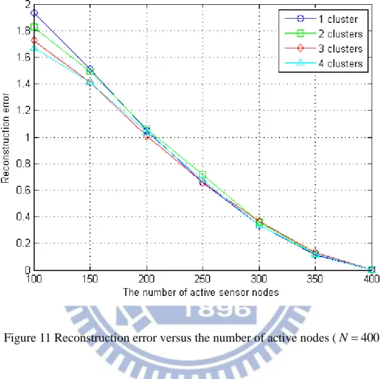
Figure 11 Reconstruction error versus the number of active nodes (N400) ... - 30 -

(8)

vi

LIST OF SYMBOLS

Symbol Definition

T The number of samples of each sensor nodes K The sparsity level

N The number of all sensor nodes M The number of active sensor nodes

p _{The transmission rate}

E The energy consumption of each sensor node R

E

The reconstruction error

Θ The combination of Φ and Ψ

Φ The measurement matrix

Ψ The transformation matrix

U The orthonormal matrix composed of the eigenvectors of Σˆ i

C

U The transformation matrix of i-th cluster

G

U

The diagonal matrix composed of _UCi ˆ

Σ The sample covariance matrix of

x

_t i



The i-th eigenvalue of Σˆ

x

The sample mean of

x

_t i

C

x The sample mean of Ci

t

x

t

y

The known dataset at given time

t



x

The received signal of active sensor nodes at given time

t

(9)

vii

i

C t

x

The original signal of sensor nodes in i-th cluster at given time

t

s

The principal component of

x

_t at given time

t

i

C t

s

The principal component of Ci

(10)

- 1 -

Chapter 1 Introduction

Machine-to-machine (M2M) [1], [2] communications are getting more and more popular in recent years. M2M communications provide the more and more convenient and highly efficient applications of life by lots of devices which connect to the network. The enormous network is composed of many machines such as computers, sensors, actuators, mobile devices, home appliances, vehicles, and etc. Thus, machine-to-machine communications is also called Internet of Things (IoT). The technology are designed for many kinds of applications such as environment monitoring, smart house, human body healthcare, vehicle safety and so on. There are four major layers in M2M communications architecture such as smart sensors collect data, transmission of select data through communication networks, compute and analysis the information, and response to the available information.

Figure 1 Architecture of M2M Communications

Application and service layer • Intelligent agent • Situation awareness Management layer • Cloud computing • Data mining • Data clustering Communication layer

• Mobile communication technologies • Wireless sensor network

• Body area network

Sensing layer

• Sensor • Actuator • RFID

(11)

- 2 -

In the near future, hundreds of thousands of wireless sensors will be deployed in our living world and provide various services and applications for us. The cost of maintaining these huge amount of sensors will be a major concern about the sensor network. One of sensor maintain cost is energy consumption. It is almost impossible to replace all batteries of those wireless sensors which are deployed in a big area. Therefore, the issue could be solved by designing a more advanced low power consumption wireless sensor, or improving the data transmission scheme to prolong the battery lifetime of the wireless sensors.

The Shannon-Nyquist sampling theorem indicates that to capture a signal of interest without missing important information, we must sample the signal at the Nyquist rate which is equal to twice the bandwidth of the signal. However, an alternative theorem which is called compressive sensing (CS) [3], [4], [5], [6] could exactly recover the original signal below the Nyquist rate. Compressive sensing is proposed by Donoho, Candes, and Tao in 2006. The innovative methodology establishes an efficient reconstruction algorithm for a small number of random linear projections of a compressible signal.

In this thesis, we focus on how to improve the data transmission scheme in the wireless sensor network. To save the energy consumption of the wireless sensor network by decreasing the transmission rate but preserving the information accuracy. In other words, consider a wireless sensor network which consists of lots of sensor nodes and a server. The sensor nodes in the wireless sensor network have two types of status, one is active mode, and the other is idle mode. When a sensor node is in active mode, it obtains the readings from the physical environment and transmits the data to the data processing center through the wireless interface. Conversely, when a sensor node is in idle mode, it just turns off

(12)

- 3 -

most of the functions for power saving and waits the control system call. The server receives all data packets of the active sensor nodes and reconstructs the data of the idle sensor node through compressive sensing technique. The reconstruction error of the recovered data must satisfy the minimum precision requirement. Thus, we could save energy by decreasing the number of the active sensor nodes, but the reconstruction error of the recovered data might raise relatively. There is a fundamental trade-off between the number of active sensor nodes and the reconstruction error.

In [12], the authors propose that compressive sensing is applied in a decentralized wireless sensor network. The actual networked data might be not sparse, but could be represented with s small number of diffusion wavelet coefficients. In [13], the authors proposed an efficient cluster-sparse reconstruction algorithm for data compression in a wireless sensor network aiming to more accurate data reconstruction and lower network energy consumption. In [14], the authors propose two algorithm which is called Universal algorithm and Gaussian algorithm respectively of finding transformation of signal to be sparse. In [15], the authors propose a compressive sensing based data gathering scheme in home area network for smart grid to demonstrate a low power data gathering design. In [16], the authors propose a clustering method that uses hybrid compressive sensing for sensor networks. The sensor nodes are organized into clusters and each clusters has a cluster head. Within a cluster, all sensor nodes transmit their data to cluster head without using compressive sensing. Then, each cluster heads use compressive sensing to transmit data to sink. The goal is to reduce the number of transmissions in the network. In [17], the authors use principal component analysis to find linear transformation that let the signal be sparse and further joint principal component analysis with compressive sensing to recover the original signal from a small number of samples. In [18], the author propose an

(13)

- 4 -

enhancement to a Bayesian estimation approach and isotonic regression approach. In [19], the authors present a complete design to apply compressive sensing for a large scale wireless sensor network. The proposed method is able to reduce global scale communication cost without introducing intensive computation or complicated transmission control.

The rest of this thesis is organized as follows. First of all, in Chapter 2, the theorem of compressive sensing is briefly introduced. Next, our proposed clustered compressive sensing scheme and the system architecture assumptions will be presented in detail in Chapter 3. Then, in Chapter 4, we evaluate the performance of our proposed methodology. Finally, this thesis makes conclusions in Chapter 5.

(14)

- 5 -

Chapter 2 Compressive Sensing

In this chapter, the theorem of compressive sensing will be briefly introduced. Compressive sensing is being believed that a sparse signal could be completely reconstructed from an underdetermined measurement. Meanwhile, the algorithm of reconstruction a sparse signal is quite simple. There are two main fundamental premises of compressive sensing, the first one is sparsity and the other one is incoherence [11]. In the following sections, we first give a quick concept of compressive sensing. Then, we explain how to design a measurement matrix for satisfying restricted isometry property. Finally, we introduce the theory of reconstruction algorithm for compressive sensing.

2.1 Overview of Compressive Sensing

The key concepts of compressive sensing is that we could perfectly reconstruct the original signal from an underdetermined measurement. Consider a real-valued, finite length, one-dimensional, discrete time signal  N

x , which could be regard as an N1 vector with entries

x

n

,

n



1, 2, ,

N

. Let



φi|i1, 2, ,N



be a set of N1 orthonormal basis

vector for the space N

. And let _Ψ N N

be an orthonormal matrix where the i-th column is the i-th basis vector

φ

_i. Any given signal could be expressed as a linear combination of these basis by

1 or N i i i s  



x φ x = Ψs (2.1)

(15)

- 6 -

, where

s

is an N1 vector of s_i  x,φ_i . Both the two vectors x and

s

are

equivalent representations of the signal. Typically, we say that x is the signal in the time

domain or spatial domain and

s

is the signal in the Ψ domain.

In general, we assume that

s

is sparse, that is, it is a linear combination of only K basis vectors.

We measure the signal x by sampling the measurement matrix Φ M N . Then, by

substituting x = Ψs into Equation (2.1) we get

y = Φx = ΦΨs = Θs, (2.2)

where Θ = ΦΨ is an MN matrix . The process of measurement is not adaptive, that is, the measurement matrix Φ is fixed and not depend on the signal x. The objective of

compressive sensing is to design a stable measurement matrix Φ to ensure that the information in a sparse or compressible signal won’t be damaged by dimensionality deduction and a reconstruction algorithm to perfectly recover the original signal from M measurements.

2.2 Measurement Matrix

In this section, we present how to design a proper measurement matrix for compressive sensing. Our goal is that to capture the most significant coefficient of the original signal and discard all the others without losing too much information. Since the measurement matrix _Φ M N

and M N, directly solving x from Equation (2.2) is completely

(16)

- 7 -

-sparse signal and the positions of the K nonzero coefficients of

s

which denotes as



i s| _i 0,i 1, 2, ,N



     are known, we could use an M K matrix

Θ

_ where M K for the purpose of restricting the positions of the nonzero coefficients of

s

. A necessary and sufficient condition for this simplified problem to be well conditioned is that, for any given K -sparse vector _ N

v which the positions of the nonzero coefficient is the same as

s

, we have

2 2 2 2 1  Θ v  1 , v (2.3)

for some  0, that is to say the matrix

Θ

_ have to preserve the lengths of these K -sparse vectors. However, generally speaking, the positions of the K nonzero coefficient are unknown. Candès et al. have shown that a sufficient condition for a stable inverse for K-sparse vectors is that  satisfies the Equation (2.3) for any arbitrary 3K -sparse vectors. The sufficient condition is referred to as the restricted isometry property (RIP) [7], [8], [9]. The restricted isometry property is defined as follows





2 2





2

2 2 2

1K x  Φx  1 K x , (2.4)

for each integer 1 K N, exist a restricted isometry constant



K



0

of a matrix Φ as a smallest number. When the restricted isometry property holds for all K-sparse vector

x, we could say that a matrix Φ has the K -restricted isometry property with the

restricted isometry constant



K if



K is not too close to one.

To design a measurement matrix Φ so that Θ = ΦΨ satisfies the restricted isometry property requires verifying all N

K

   

(17)

- 8 -

approach to design a measurement matrix Φ which could simply achieve the restricted isometry property and incoherence is to choose the measurement matrix Φ as a random matrix. The MN random matrix could be obtained according the following way: 1) by sampling N i.i.d. entries from normal distribution with mean 0 and variance 1

M ,

and 2) by sampling N i.i.d entries form symmetric Bernoulli distribution

, 1 1 2 i j P M    _ _   _ _ 

 . All the matrices obey the restricted isometry property provided

that log N M C K K     _{ }   (2.5)

where C is a small constant.

2.3 Reconstruction Algorithm

The most impressive thing is that the algorithm for signal reconstruction of compressive sensing could be easily obtained by convex optimization. To recover the original signal, we must take the M measurements in the received signal

y

, the measurement matrix

Φ, and the transformation matrix Ψ and reconstruct the N -dimensional original signal x or, equivalently, its sparse representation s. Since the number of measurements

is much smaller than the dimension of the original signal, recovering x from

y

is an

ill-posed problem. There might be hundreds of thousands of s that satisfy Equation (2.2),

(18)

- 9 -

could be guaranteed. Fortunately, we already know that s is sparse, we could restrict the

number of nonzero entries in vector s , that is

0

min , subject to

s s y = Θs. (2.6)

The above optimization problem could be solved by greedy algorithms such as orthogonal matching pursuit (OMP) [20] or compressive sampling matching pursuit (CoSaMP) [21]. In greedy algorithm, set x0 and the residual r x

 

in the beginning. Next, in each iteration, the atom that most correlated to the residual r x

 

is added into the support set and then x is updated by solving the least-squares problem by using the support set.

Finally, the iteration stop when the number of select atoms is equal to K. However,

0

min

s s is not convex and thus the convergence to the global optimum is hard

to be ensured for greedy algorithms. Candès et al. has proven that when the restricted isometry property of the measurement matrix Φ satisfies certain conditions or the measurement matrix Φ is incoherent to the transformation matrix Ψ, the original signal

s

could be recovered by ₁ norm minimization as follows

1

min subject to

s s y = Θs (2.7)

Obviously, the above optimization problem is convex and have the global optimum, which could exactly recover a sparse or compressible signal with high probability. Many algorithms have been proposed to solve the convex optimization problem, including basis pursuit (BP) and linear programming (LP) [10].

(19)

- 10 -

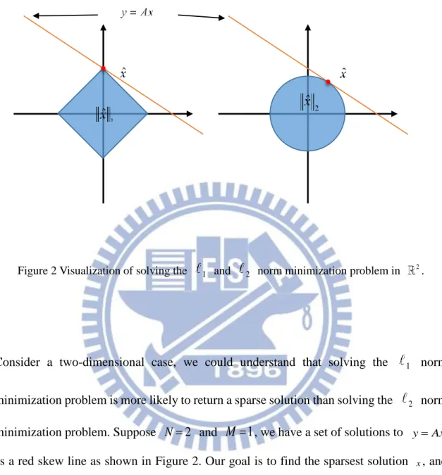
Figure 2 Visualization of solving the 1 and 2 norm minimization problem in 2.

Consider a two-dimensional case, we could understand that solving the ₁ norm

minimization problem is more likely to return a sparse solution than solving the ₂ norm

minimization problem. Suppose N2 and M 1, we have a set of solutions to yAx

as a red skew line as shown in Figure 2. Our goal is to find the sparsest solution x, and

apparently, x is 1-sparse in this case. Each blue region represents the minimum value of

1

x and x ₂ as ₁ball and ₂ ball respectively. The minimizing ˆx ₂ subject to ˆ

yAx returns the solution that closest to the origin but the solution is not a sparse solution. The only way of the solution to be a sparse solution is that if the line of solutions is parallel with one of the axes, which happens if and only if one of the entries of A is zeros. However, the minimizing ˆx₁ subject to yAxˆ gives a sparse solution when

(20)

- 11 -

the line of solutions touch at the corner of the 1 ball. The line of solutions might overlap

with the one of the edges of the ₁ ball, which happens if A 





 





1 2 . Furthermore, we could intuitively extend this kind of problem into higher dimensions.

(21)

- 12 -

Chapter 3 Clustered Compressive Sensing

In this chapter, we first introduce the system architecture of the wireless sensor network and related assumptions. Next, we introduce a technique which joint principal component analysis (PCA) and compressive sensing, which is published by Masiero et al. in 2009 [17]. Finally, we propose a methodology of combining clustering and compressive sensing. We call the method as clustered compressive sensing.

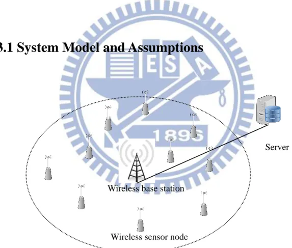
3.1 System Model and Assumptions

Figure 3 the wireless sensor network model.

Server

Wireless base station

(22)

- 13 -

In our scenarios, the wireless sensor network system consists of one server for computing and storing information and N autonomous sensor nodes for collecting data of physical environment. Meanwhile, we assume all of the N sensor nodes are uniformly and independently distributed in a region of various terrains. And we also assume that all of the N sensor nodes collect data by following the same transmission rate in a synchronized time slot. Once a sensor node obtains its reading of physical environment in a time slot, the sensor node immediately transmits the data packet to the server through the wireless interface in the same time slot. Each of the N sensor nodes has two types of status, one is active mode and the other one is idle mode. In active mode, a sensor node takes the actions of sensing the physical environment and transmitting the data packets to the server through the wireless interface, on the other hand, a sensor node in idle mode turns off most of functions to reduce energy consumption. Supposed that a sensor node in active mode consumes most of energy and the energy consumption in idle mode is too small to ignore, the energy consumption of a sensor node is viewed as E. The maximum energy consumption of the wireless sensor network is N E , while all of the N sensor nodes are in active mode and the energy consumption of the server and the wireless base station is not include. Therefore, we can decrease the number of active sensor nodes by adjusting the transmission rate to reduce the energy consumption. Let only M active sensor nodes in each time slot, and the energy consumption could be represented as

M E . Also, the transmission rate could be viewed as p M N

 .Of course, the other NM sensor nodes are in idle mode and their data could be recovered by the reconstruction algorithm of compressive sensing. The reconstruction error must meet the system minimum precision requirement. As the result, there is a trade-off between energy

(23)

- 14 -

consumption and reconstruction error. In the following section 3.2, we will briefly introduce how to recover the missing data from known information.

Furthermore, generally speaking, the physical environment is various in many places. For example, the quality of groundwater of Hsinchu City, the quality is the best in mountain area, good in downtown and the worst in industrial districts. Suppose we would like to monitor the quality of groundwater of the whole city by installing numerous of sensors underground and gathering those readings of sensors. Since the data of a specific area has its characteristic and distribution, we could assign the sensors which have similar characteristics or follow the same distribution into a cluster. Then, we could look for a sparsest representation of each clusters. It seems easier to find a sparse representation of each clusters than that of all the data. Therefore, suppose that to observe a region of various environment by a wireless sensor network. Let x



x x₁, ₂, ,x_N



T,x N denotes a vector of original data collected from all of the N sensor nodes and

x n

_n

,



1, 2, ,

N

is the readings of physical environment of each sensor nodes. Assume that x is comprised

of several distributions and the sensor nodes whose readings belong to the same distribution are close to each other. Our major target is that to find out the sparsest representation of signal x, therefore, we come up with an idea that to divided those sensor

nodes into clusters according to their readings and geographic positions, in this way, we might obtain the more sparse representation of the subset of signal x.

(24)

- 15 -

3.2 Joint PCA and CS

Suppose that to collect all readings from a wireless sensor network with N sensor nodes, according to a fixed sampling rate at a discrete time t1, 2, ,T. Let

x

_t



N be a vector of the readings collected from all sensor node at a given time

t

. In geometric point of view,

x

t could be viewed as a single point in N surface and we are looking for vector

s

t in K -dimensional plane



KN



which provides the best fit of

x

t in terms of minimum the Euclidean distance. The projection of

x

t into

 K t s could be defined as  K def T

_

_

t  K t s U x x , (3.1)

where

U

_K is an NK orthonormal matrix whose the column vectors consists of K eigenvectors which is corresponding to the K largest eigenvalues of covariance matrix of

x

t and

x

is the mean of

x

t. The mean vector and the covariance matrix could be replaced by the sample mean vector

x

and the sample covariance matrix Σˆ as

1 1 T t t T  



x x , (3.2)







1 1 ˆ 1 T T t t t T     



Σ x x x x . (3.3)

(25)

- 16 -





ˆ T

t   K t   K K t 

x x U s x U U x x . (3.4)

Furthermore, we apply the principal component analysis methodology to compressive sensing. In compressive sensing, we would like to reconstruct a given signal x from

receiving a small number of measurements M , which is much smaller then N . In a wireless sensor network with N sensor nodes, suppose we only collect the packets of the M active nodes at each time

t

, the set of the M packets could be represented as a vector form

x



_t. The M active nodes are chosen randomly from the N sensor nodes by an MN routing matrix



. Thus, the relationship between

x

_m and

x



_m could be written as

t t



x = Φx

. (3.5) According to the principal component analysis scheme, we could represent the sparse vector

s

_t



s

(_tN) at each time

t

as





T

t  N t

s U x x (3.6)

Suppose that

x

_t could be completely obtained from s _tK by applying Equation (3.4), we could say that

s

_t is a K-sparse vector as

  0 K t t N K        s s , (3.7)

(26)

- 17 -

where

0

N K is a



NK



1 vector with all zero entries. Because

U

N is an orthonormal matrix, we have

I

_N



U U

_N T_N , where

I

N is an NN identity matrix. Thus, the Equation (3.6) could be rewritten as

t

 

N t



t

x

x U s

Ψs

(3.8) where the transformation matrix Ψ is totally equal to

U

_N. By combining Equation (3.5) and Equation (3.8) we could write





t t t t

    

x Φx Φ x x ΦΨs = Θs . (3.9)

Since the form of Equation (3.9) is similar to that of Equation (2.2), we could easily apply the compressive sensing reconstruction algorithm to recover a good estimate of

s

_t, denoted as

s

ˆ

_t. Once

s

ˆ

_t is obtained,

x

_t would be recovered from

s

ˆ

_t according to Equation (3.4), as

ˆ

_t



_t



x

Ψs x

(3.10)

(27)

- 18 -

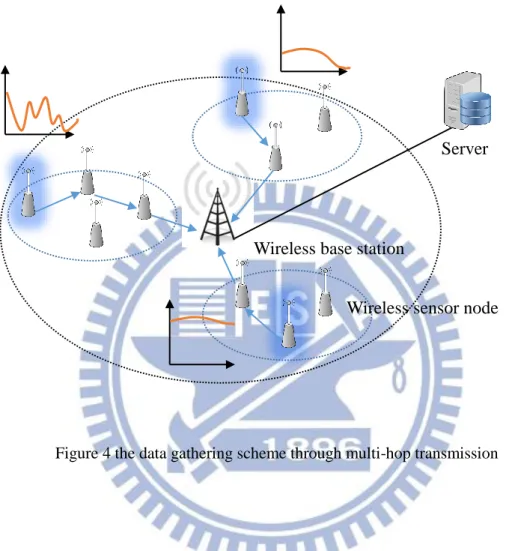
3.3 Clustered Compressive Sensing

Figure 4 the data gathering scheme through multi-hop transmission

In this section, we propose a methodology of clustering and combining compressive sensing. Our goal is to recover the length- N original signal from M active nodes. To achieve this goal, we must collect some prior knowledge of this network. We use k-means clustering methodology to divide those sensor nodes into clusters according to the readings of those sensor nodes. In each cluster, the data might be more similar to each other, thus we could use principal component analysis for each of clusters. In this way, we could get the more sparse representation s of x, that is to say, we could collect less data of those

sensor nodes, but we still could recover the whole data of x. We could consider this

Server

Wireless base station

(28)

- 19 -

methodology as a two-step reduction of signal dimensions. The first step is that the similar information into the same group, and further use principal component analysis of each of the clusters.

For example, suppose all sensor node are divided into three clusters as follows

1 2 3 C t C t t C t            x x x x (3.11)

The next step, we apply principal component analysis to each of the clusters. That is

1 1 1 1 2 2 2 2 3 3 3 3 , , . t t t t t t C C C C C C C C C C C C       x x U s x x U s x x U s (3.12)

Then, by combining (3.11) and (3.12), we have

1 1 1 2 2 2 3 3 3 1 1 1 2 2 2 3 3 3 1 1 1 2 2 2 3 3 3 0 0 0 0 0 0 t t t t t t t t t C C C C C C t C C C C C C C C C C C C C C C C C C C C C      _  _  _            _ _{ } _                     _ _{ } _{  }             x U s x x U s x U s x U s x U s x U s x U s x U s x U s (3.13)

Furthermore, we define U_G is a diagonal matrix which the diagonal entries is composed

of _UC1, _UC2, and _UC3. We could rewrite Equation (3.13) as

t

 

G t

(29)

- 20 -

Thus, we need to ensure that U_G is still an orthonormal matrix by

1 1 2 2 3 3 1 1 2 2 3 3 1 1 2 2 3 3 0 0 0 0 0 0 0 0 0 0 0 0 0 0 0 0 0 0 0 0 0 0 0 0 0 0 0 0 0 0 0 0 0 0 0 0 T C C C C T G G C C C C T C C T C C T C C T C C T C C T                                                                  U U U U U U U U U U U U U U U U U U U U I I I I (3.15)

(30)

- 21 -

Chapter 4 Performance Evaluation

In this chapter, we study the effectiveness of our proposed clustered compressive sensing and evaluate the performance by calculating the reconstruction error between the original signal and the recovered signal. We consider a wireless sensor network with N sensor nodes is employed in a square region of side D units, which is evenly divided into N small square grids. All of the N sensor nodes are uniformly distributed in this region so that each grids has only exactly one sensor node. Each of the N sensor nodes could only communicate with all other sensor nodes in a circular range of radius R units. Since RD, each of the N sensor nodes transmits its data packets through multi-hop connections. All of the data packets will be concentrated to the processing server eventually. The wireless base station is placed in the center of this region and connects with the server through cable connection. The server is in charge of data storing and processing including data clustering and principal component analysis.

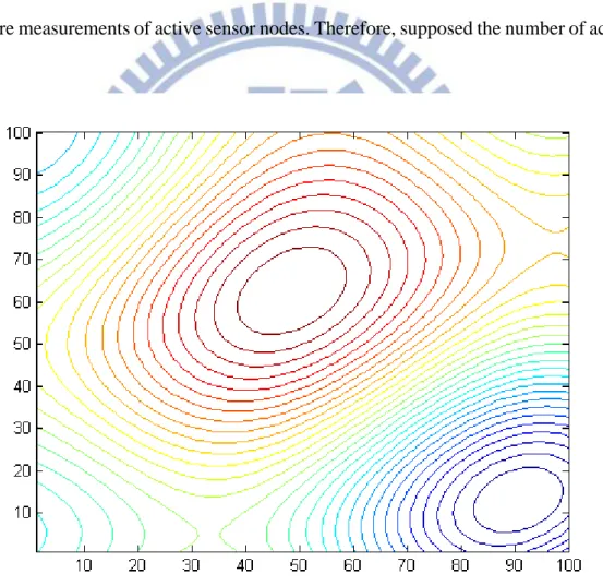
The input signal is a simulated temperature distribution in a square region which is separated into four regions. The simulated temperature distribution in each sub-regions is different to each other. In each sub-sub-regions, the simulated temperature is a

2 2

D_D

square matrix

T

_g

,

g



1, 2,3, 4

with 2

4

D

elements, where elements

, | 1, 2, , , 1, 2, , 2 2 i j D D t i j  _ _   

  are the value of simulated temperature and spatially

correlated. The simulated temperature generation procedure is executed as the following steps:

(31)

- 22 - 1) we start from a 2 2 D_D matrix

H

_g

, g 1, 2,3, 4



with 2 4 D

entries, where entries







hi j, |i j | 5  15,  



are generated from continuous uniform

distribution;

2)

T

_G is obtained from

H

_G by inversing discrete cosine transformation;

3) sampling the data correspond to the positions of all N sensor nodes, thus we simulated temperature signal

x

t;

(32)

- 23 -

4) finally, in order to verify the robustness of our proposed methodology, we add an i.i.d. random Gaussian noise w



0,2



into all entries of signal

x

t.

The simulated temperature model is shown in Figure 5.

To implement our proposed clustered compressive sensing methodology, we alternate two phases as below. One is training phase and the other one is monitoring phase. In training phase, first of all, T samples of each sensor nodes are collected into the server. Next, all

(33)

- 24 -

of the N sensor nodes are divided into G clusters according to their positions because we consider that the readings of those adjacent sensor nodes are similar substantially. We allocate the collected data into clusters according to their cluster indices. Then, each cluster apply the principal component analysis to obtain its sample mean and sample covariance. And finally, merge those sample mean into a longer vector and form those sample covariance into a diagonal matrix.

Subsequently, in monitoring phase, we randomly select M active sensor nodes from N sensor nodes. The data of the other NM sensor nodes is reconstructed from the subset of input signal by using the sample mean and sample covariance which is calculated in training phase.

To evaluate the performance of proposed methodology, we consider an indicator such as the reconstruction error.





1 1 N _ˆ R i i i E x x N  



 (4.1)

where

x

is the original signal, and ˆx is the approximated recovered signal. All of the simulations have been performed under the following platform: MATLAB R2011b on a computer with Intel Core i5 661 3.33GHz CPU, 8GB RAM, and Windows 7.

(34)

- 25 -  Scenario 1

In Scenario 1, we consider that there is only one distribution of the input signal and the number of sensor nodes N100 in the wireless sensor network. The simulated temperature model is shown in Figure 6. Figure 7 shows that the relationship between reconstruction error and the number of active nodes. Since only one distribution in this region, choose one cluster is the best idea. When choose more than one cluster, the sparsity level is getting higher. Thus, for higher the sparsity level, we must need more measurements of active sensor nodes. Therefore, supposed the number of active

(35)

- 26 -

sensor nodes is the same, choose four clusters has the highest reconstruction error, on the other hand, choose one cluster has the lower reconstruction error. As the result, it is not necessary that allocating those sensor into clusters when the environment is follow simple distributions.

(36)

- 27 -  Scenario 2

In scenario 2, we consider that there are four distributions of the input signal. The input signal is shown in Figure 5, and the number of sensor nodes N100. In Figure 9, we can clearly understand that for using four clusters, each of the distribution might have the best fit. Obviously, the reconstruction error for four clusters is the smallest.

(37)

- 28 -

Thus, the sparsity must be the smallest as shown in Figure 10 and when the number of cluster decrease, the higher the sparsity level need.

(38)

- 29 -

However, according to Equation (2.5) and the restricted isometry property, we must need at least 3K measurements, thus the signal could be recovered perfectly. In

44

K case, the necessarily measurement M 132, therefore, using N100 is not enough to completely reconstruct the original signal. Furthermore, we employ

400

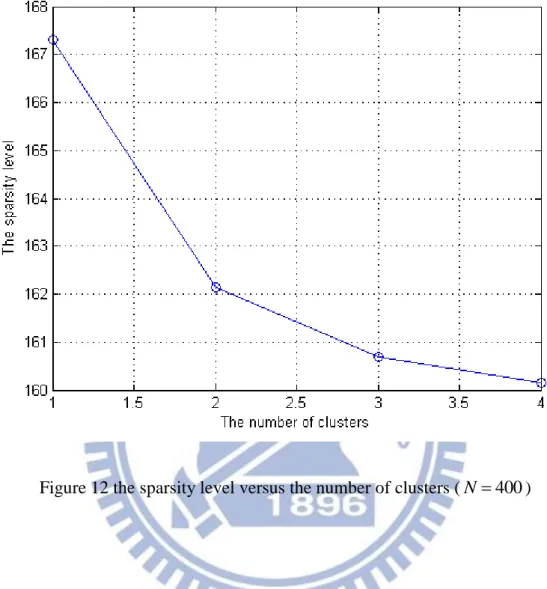
N  sensor nodes into this region. The result is shown in Figure 11 and the sparsity level is shown in Figure 12. As we can see that the sparsity level become

(39)

- 30 - 160

K  , according to the restricted isometry property, N 400 is still not high enough to perfectly recover the original signal. but the total reconstruction error is lower than N 100, as the result, supposed that we could endure the temperature has the mean square error is equal to 0.1, we could choose four clusters for only need

(40)

- 31 -

about 350 active sensor nodes, on the contract side, if we choose one cluster, we need near 370 active nodes.

(41)

- 32 -

Finally, for a multi-environment region, it is hard to find the sparsest representation of the original by using principal component analysis, but in a monotonous environment, it is quiet easier than multi-environment. Although, we could not perfectly recover the original signal, we still could regard the approximation signal as a reference when the reconstruction error is satisfied the minimum precision requirement.

(42)

- 33 -

Chapter 5 Conclusion

In this thesis, we present a joint design of clustering and compressive sensing for a wireless sensor network which is deployed in a wide region with a variety of environments. This proposed methodology is aim to recover the data of the unreceived sensor nodes from that of the received sensor nodes. By clustering those sensor nodes, we could reduce the complexity of the input signal, and we could further find out the more sparse representation of the input signal. The less the sparsity level the original signal has, the less number of active sensor nodes need and the less energy of idle sensor nodes consume. As the result, we could make a trade-off between reconstruction error and energy consumption.

From the performance simulation, we evaluate the differences between uni-environment region and multi-environment region. In the uni-environment region, we could easily find out the sparsest representation of the original signal, and it is not necessary that to divided all sensor nodes into clusters. On the other hand, in multi-environment region, separating those sensor nodes into clusters could efficient reduce the reconstruction error, thus we could assign less active sensor nodes to transmit its readings of physical environment to save more energy. However, the sparsity level in multi-environment region is unsatisfactory. Since we increase the total number of sensor nodes, it is still not able to recover the original signal perfectly.

(43)

- 34 -

Therefore, in future work, we must have to find out a more efficient method to let the original signal has the sparsest representation in various environments area. Maybe we can not only use principal component analysis to find the sparsest representation but also apply another approach into compressive sensing. We can use different approaches for each clusters according to the characteristics or distributions of the data of each clusters. Furthermore, we can improve our clustering methodology, because in this thesis we just use k-means clustering according to the geographic position of the sensor nodes. Thus, how to cluster those sensor nodes intelligently and efficiently can be the next major issue.

(44)

- 35 -

REFERENCE

[1] Y. Chen, “Challenges and opportunities of internet of things,” 2012 17th Asia and South Pacific Design Automation Conference (ASP-DAC), pp 383-388, Jan 2012

[2] M. Chen, J. Wan, and F. Li, “Machine-to-machine communications: architectures, standards, and applications,” KSII Transactions on Internet and Information Systems, vol. 6, no. 2, pp. 480-497, Feb. 2012

[3] D. Donoho, “Compressed sensing,” IEEE Transactions on Information Theory, vol. 52, no. 4, pp. 1289-1306, April 2006

[4] E. Candès, “Compressive sampling,” International Congress of Mathematicians, vol. 3, pp. 1433-1452, Aug. 2006

[5] E. Candès, and M. Wakin, “An Introduction to Compressive Sampling,” IEEE Signal Processing Magazine, vol. 25, no. 2, pp.21-30, March 2008

[6] R. Baraniuk, “Compressive Sensing (Lecture Notes),” IEEE Signal Processing Magazine, vol. 24, no. 4, pp.118-121, July 2007

[7] E. Candès, and T. Tao, “Decoding by linear programming,” IEEE Transactions on Information Theory, vol. 51, no. 12, pp. 4203-4215, Dec. 2005

[8] E. Candès, J. Romberg, and T. Tao, “Robust uncertainty principles: exact signal reconstruction from highly incomplete frequency information,” IEEE Transactions on Information Theory, vol. 52, no. 2, pp. 489-509, Feb. 2006

(45)

- 36 -

[9] E. Candès, J. Romberg, and T. Tao, “Stable signal recovery from incomplete and inaccurate measurements,” Communications on Pure and Applied Mathematics, vol. 59, no. 8, pp. 1207-1223, Aug. 2006

[10] E. Candès, and T. Tao, “Near-Optimal Signal Recovery From Random Projections: Universal Encoding Strategies? ,” IEEE Transactions on Information Theory, vol. 52, no. 12, pp. 5406-5425, Dec. 2006

[11] E. Candès and J. Romberg, “Sparsity and incoherence in compressive sampling,” Inverse Problems, vol. 23, no. 3, pp.969-985, April 2007

[12] J. Haupt, W. Bajwa, M. Rabbat, and R. Nowak, “Compressed Sensing for Networked Data,” IEEE Signal Processing Magazine, vol. 25, no. 2, pp. 92-101, March 2008 [13] S. Li, L. Xu, and X. Wang, “Compressed Sensing Signal and Data Acquisition in

Wireless Sensor Networks and Internet of Things,” IEEE Transactions on Industrial Informatics, vol. 9, no. 4, pp. 2177-2186, Nov. 2013

[14] G. Chen, H. Yang, and L. Huang, “Optimizing Compressive Sensing in the Internet of Things,” in Y. Zhang eds. Future Wireless Networks and Information Systems, pp. 253-262, Springer Berlin Heidelberg, 2012

[15] T. Islam, and I. Koo, “Compressed Sensing-based data gathering in wireless Home Area Network for smart grid,” 2012 International Conference on Informatics, Electronics & Vision (ICIEV), pp.82-86, May 2012

(46)

- 37 -

[16] R. Xie, and X. Jia, “Transmission Efficient Clustering Method for Wireless Sensor Networks using Compressive Sensing,” IEEE Transactions on Parallel and Distributed Systems, vol. PP, no. 99, pp. 1-10, March 2013

[17] R. Masiero, G. Quer, D. Munaretto, M. Rossi, J. Widmer, and M. Zorzi, “Data Acquisition through Joint Compressive Sensing and Principal Component Analysis,” 2009 IEEE Global Telecommunications Conference, pp.1-6, Dec. 2009

[18] D. Hu, S. Mao, and N. Billor, “On balancing energy efficiency and estimation error in compressed sensing,” 2012 IEEE Global Communications Conference, pp. 4278-4283. Dec. 2012

[19] C. Luo, F. Wu, and J. Sun, “Compressive data gathering for large-scale wireless sensor networks,” in Proceedings of the 15th annual international conference on Mobile computing and networking, pp.145-156, Sep. 2009

[20] J. Tropp and A. Gilbert, “Signal Recovery From Random Measurements Via Orthogonal Matching Pursuit,” IEEE Transactions on Information Theory, vol. 53, no. 12, pp. 4655-4666, Dec.2007

[21] D. Needell and J. Tropp, “CoSaMP: iterative signal recovery from incomplete and inaccurate samples,” Applied and Computational Harmonic Analysis, vol. 26, no. 3, pp. 301-321, May 2009

針對物聯網之群集壓縮感知技術

國立交通大學

電子工程學系電子研究所碩士班

碩士論文