B. J. Huang Professor.
s. c. nil
Graduate Assistant. Department of Mechanical Engineering, National Taiwan University, Taipei, Taiwan 10764
A Performance Test Method of
Solar Thermosyphon Systems
A method of test for the thermal performance rating of thermosyphon systems is developed in the present study. It is suggested that the overall performance rating of a solar thermosyphon system should include (1) system efficiency test during the energy collecting phase and (2) system cooling loss test during the cooling phase. Both the tests are performed outdoors. The cooling loss test is performed right after the efficiency test. A semiempirical system efficiency model with a variable (T; -Ta)/Ht is derived to correlate the daily efficiency test results; while a simple
first-order model with a cooling time constant TC is used to evaluate the loss parameter
in cooling phase. A method of test is then proposed and an expert system is designed to perform the outdoor tests. It is shown that very good correlation for the system efficiency model is obtained and the system parameters obtained can be used to rate the thermal performance in energy collecting phase; while the thermal performance
in cooling phase is rated by examining the time constant TC of the cooling loss model.
1 Introduction
The thermal performance of solar thermosyphon systems is affected by system design parameters and operating conditions. The system design parameters include thermal properties and surface area of collector, size and length of connecting pipes, tank volume, insulation design, and geometric configuration of the system, etc. The operating conditions include solar ir-radiation incident upon the collector slope, operating temper-ature range, ambient conditions, and hot-water load pattern, etc. The system performance usually behaves as a stochastic process due to random variations of solar irradiation, ambient temperature, wind speed/direction, and hot-water load pat-tern, etc. This makes the derivation of a system performance model quite difficult, and a test method or standard for thermal performance rating of solar thermosyphon systems has not yet been established very well.
Several test methods based on a long-term or short-term monitoring of different solar thermosyphon systems have been proposed (Fanny, 1984; Beale, 1987). However, the simplest or probably the best test method for a thermosyphon system would be the outdoor daily efficiency test performed under various climatic conditions. That is, the test is performed con-tinuously over a finite time period and records the daily total irradiation incident upon the collector slope, the average am-bient temperature and wind speed, the initial and final water temperatures in the tank, etc. The daily efficiencies are then calculated and used to fit a system performance model to determine the system parameters. The present study intends to develop a test method based on the daily efficiency test results.
In addition to the energy collecting efficiency at daytime, Contributed by the Solar Energy Division of THE AMERICAN SOCIETY OF MECHANICAL ENGINEERS for publication in the JOURNAL OF SOLAR ENERGY E N -GINEERING. Manuscript received by the ASME Solar Energy Division, Jan. 3, 1990; final revision, Apr. 2, 1991.
cooling loss after sunset or during cloudy periods in daytime is also an important factor in evaluating a solar thermosyphon system. Therefore, a system cooling loss test should also be conducted. The system cooling loss of a solar thermosyphon system results mainly from convection loss of the storage tank. However, if the system design is not proper, an additional cooling loss from collector will result due to flow reversal (i.e., the collector becomes an energy radiator). To rate the system cooling loss, a cooling loss test should be performed right after the daily efficiency test. The test results are then used to fit a system cooling loss model to determine the cooling loss pa-rameters.
From the foregoing discussion, it can be seen that a thorough performance test of a solar thermosyphon system should in-clude: (1) system efficiency test during the energy collecting phase; and (2) system cooling loss test during the cooling phase. An attempt is made in the present study to derive the system performance models for the energy collecting and the system cooling loss phases. Then, a test method for thermal perform-ance rating of solar thermosyphon systems is developed. An expert system is also designed for the outdoor testing.
2 System Efficiency Model in Energy Collecting Phase 2.1 Basic Assumptions. The hot-water load pattern
im-posed during the energy collecting phase is quite a complicated factor affecting the system performance (Morrison and Saps-ford, 1983; Morrison and Tran, 1984). Standardizing the hot-water load pattern in the performance test can be a solution to this problem. But, it may not be feasible since the selection of a standard load pattern is difficult. Recently, Morrison and Tran (1988) developed a test method which considers the hot-water load. However, it is shown that the variation of daily loads should be small in order to assure a good correlation.
Besides, the major disadvantage of this test method is that two to three months testing is required.
It is noticed that the efficiency of a thermosyphon system with morning peak-load pattern is higher than that with after-noon peak load (Morrison and Sapsford, 1983). As far as the system efficiency is concerned, the daily efficiency at no hot-water load during the energy collecting phase can be treated as the lower bound of the performance. Hence, in order to simplify the performance test, it is assumed that no hot-water load will be imposed during the energy collecting phase.
In the development of a system efficiency model, the fol-lowing assumptions, depending on Close's one-node model (Close, 1962), were made:
1 The temperature of the whole system can be represented by a system mean temperature.
2 The system mean temperature equals the mean water temperature in the tank.
3 Neglect the heat capacity effect of the constructing ma-terial of the thermosyphon system.
2.2 Energy Balance. In deriving a performance model based upon the daily efficiency test results, the instantaneous system performance has to be integrated over the whole energy collecting period, i.e., from sunrise to sunset. Thus, taking energy balance to the whole system and integrating for a whole day and ignoring the heat capacity effect of the system, we obtain
Qnet =Qc~ Gloss > ( 1 ) where <2net is the daily net energy collection which can be
expressed as
Q«t = MCp(T/-Tl); (2)
Qc is the daily total energy absorbed by the collector which
can be assumed to be proportional to the daily irradiation incident upon the collector slope H, and the collector area Ac,
i.e.,
Qe = aeAcHl (3)
where ae is a proportionality constant representing the effective
absorption coefficient of the system and H, is expressed as
H,= \ Ijdt (4)
I
where t, and tf are the initial and final time during energy collecting period; Qloss is the daily total heat loss which can be assumed to be proportional to the difference between the mean tank temperature and the ambient temperatures T - Ta, i.e.,
Q\™=Ut(T-Ta) (5)
where U, is a proportionality constant. For simplification, we further assume that the daily mean system temperature T can be taken as the arithmetic mean of the initial and the final temperatures, i.e.,
T=- (6)
From Eqs. (2), (3), and (5), energy Eq. (1), based on per unit collector area, can be written as,
(7)
where Us = U,/Ac. Furthermore, dividing Eq. (7) by H„ we
obtain a daily system efficiency relation: T-Ta Vs
<7net •U,
H, (8)
2.3 System Efficiency Model. The daily system efficiency relation, Eq. (8), is still not suitable since the daily mean tem-perature T is a function of irradiation H, and initial temper-ature Th as can be seen from the fact that the final temperature Tj is affected by H, and Th according to Eq. (6). A further
modification is thus necessary.
It has been noted from field experiences that the daily tem-perature rise in the tank 7} - 7) can be assumed to be pro-portional to the daily total irradiation incident on the collector slope H, (Kubler et al., 1988; Adnot et al., 1988) and the collector area Ac, but inversely proportional to the total mass
of water contained in the tank M. That is
7>-r,-fr
HM tAc (9)where b is a proportionality constant. Thus, combining Eqs. (9) with (6) we obtain - Tj+Tf Tj+Tj+bHtAc/M bHtA J~ 2 ~ 2 ~ 2M +Ih U U ) N o m e n c l a t u r e b H, It M Qc Wloss G n e t <7net collector area, m
proportionality constant defined in Eq. (9) heat capacity of water, 0.004184 MJ/kg°C daily total solar irradiation incident upon collec-tor slope, MJ/m2 day
solar irradiation incident upon collector slope, W/m2
total mass of water in the thermosyphon system, kg
daily total energy absorption, MJ/day daily total energy loss, MJ/day
daily total net energy absorption, MJ/day daily total net energy absorption per collector area, M J / m2 day
tank temperature, °C
T,f =
T
T = daily mean tank temperature Ti+T, f Ta = ambient temperature, °C
Ta = mean ambient temperature, °C Tj = initial tank temperature, °C Tf = final tank temperature, °C
TLi = initial mean tank temperature in system cooling
phase, °C
ti tf tL
u,
final mean tank temperature in system cooling phase, °C
initial time of energy collecting phase, hr final time of energy collecting phase, hr test period of cooling phase, hr
coefficient of overall system loss rate, defined in Eq. (7), M J / m2 oC day
coefficient of total heat loss, defined in Eq. (5), M J / ° C day
(C//4)o = average heat loss coefficient for isolated tank in cooling phase, W / ° C
(UA)t = overall cooling loss coefficient in cooling phase,
W / ° C
mean wind speed during test period, m/s operation parameter defined in Eq. (17), "C m2 day/MJ
effective solar absorptance, dimensionless overall solar absorptance defined in Eq. (13), di-mensionless
system cooling time constant, day
system cooling time constant for isolated tank, day
vw X ae
r0
Therefore,
T-Ta bAc T,-T„
(ID H, 2M H,
Substituting Eq. (11) into Eq. (8), we obtain the system efficiency model: Ti-Ta ris = ot0-Us H, where a0 = cxe -(M/Ac) bUs 2 (12) (13)
an and Us are the parameters of the model which depend upon
the properties of the solar thermosyphon system. Equation (12) can be used to correlate the daily system efficiency with the operating conditions through the variable (7,— Ta)/Ht. a0 and Us are to be determined from linear regression analysis
using daily efficiency test results.
a0 can also be interpreted as the system efficiency under the condition that the initial temperature 7, equals the mean am-bient temperature 7a; Us is the energy loss coefficient in the
energy collecting phase. It should be noted that Eq. (12) is a semi-empirical system efficiency model which is derived based on some assumptions. The validity of the system efficiency model, Eq. (12), thus needs experimental verification.
3 Cooling Loss Model in Cooling Phase
For simplification, a first-order system cooling loss model is used:
MQ dT(t)
dt (UA)t[T(t)-Ta], (14)
where (UA), is the overall system cooling-loss coefficient. The solution of Eq. (14) with constant coefficient {UA), is
In Tu-Ta
Tr
(15)
where TLi = 7(0) is the initial mean tank temperature in the
cooling phase; 7 y = T(tL) is the final mean tank temperature; tL is the time period for the cooling loss test; TC is the system
cooling-time constant defined as MCP
(UA) (16)
The time constant TC represents the time at which the
dif-ference between the hot water temperature in the tank and the mean ambient temperature has dropped to 36.8 percent by a cooling effect. It also represents the insulation capability of the thermosyphon system.
Equation (14) or (15) is a system cooling-loss model in the cooling phase to account for the cooling losses after sunset or during cloudy periods in daytime. The system cooling loss is mainly due to heat conduction/convection or radiation loss from the storage tank to the ambient. However, under certain circumstances, cooling loss can also be induced from the col-lector to the ambient due to flow reversal phenomenon (Mor-rison, 1985). Nevertheless, the system cooling time constant TC
is defined to include both types of heat losses and thus can be used to evaluate the overall system cooling effect.
4 Expert System Design and Setup
It has been mentioned that the outdoor test of solar ther-mosyphon systems can be divided into two parts: (1) system efficiency test during the energy collecting phase; and (2) sys-tem cooling loss test during the cooling phase. The cooling loss test should be performed right after the system efficiency
test. Since both the tests have to be performed continuously from early in the morning until late night, manual operation is inefficient and almost impossible. An expert testing system is thus developed in the present study so that the test is fully automatic. The expert system is designed to be able to run the performance tests of six different solar thermosyphon systems simultaneously.
The testing equipment of the expert system consists of: (1) a data acquisition system AD500, including a HP3456A mul-timeter for detection of sensor signals; (2) a solenoidal valve installed in the water make-up line to control the cold water inflow to adjust the initial tank temperature 7,; (3) a 1/4-hp water mixing pump used to recirculate the water from the tank in order that the thermal stratification in the tank can be completely destroyed as is required before measuring the mean tank temperature; (4) an electric timer used to turn on the whole expert system in the morning and off at late night when the cooling phase test is finished; (5) several sensors including a PSP pyranometer to measure the irradiation incident upon the collector slope, RTD probes used to measure the tank and ambient temperatures, a three-cup wind meter used to measure the wind speed; (6) a P C / A T used as the CPU of the expert system.
The initial tank temperature 7, is regulated daily early in the morning by mixing the warm water left in the tank with cold make-up water. By adjusting the time duration of the inflow of make-up water using a solenoidal valve, a desired initial tank temperature can be easily obtained.
It is noted that the water temperature in the tank is usually not uniform due to thermal stratification. This causes difficulty in measuring the average tank temperature during the system efficiency and the cooling loss tests. In fact, the average tank temperature can hardly be measured accurately even if a large number of temperature probes are installed. To overcome this problem, a mixing pump, which is connected to the tank sep-arately, is used to recirculate the water in the tank so that the thermal stratification can be completely destroyed within a short period by the mixing generated by a large recirculation flow. The mixing process is carried out by the P C / A T every time when the measurement of the average tank temperature is required.
As the thermal stratification is completely destroyed by re-circulation, the average tank temperature can be easily meas-ured by sampling at any point in the tank. To assure better results, four RTD temperature probes were installed inside the tank. However, the recirculation flow rate should be carefully controlled in order to reduce the heat loss during the mixing process. It is found that the heat loss is negligible ( < 0 . 9 per-cent) with recirculation flowrate 40 1/min for two minutes. The average tank temperature is measured by taking the av-erage readings of the 4 RTD probes installed in the tank. In general, recirculation of one minute with 40 I/min will bring the four temperature readings close enough (within 1°C).
To assure the accuracy of test results, the RTD temperature probes were calibrated against a HP2804A quartz precise ther-mometer to give an uncertainty ±0.3°C. The uncertainty of an Eppley PSP pyranometer is ±2.5 percent (given by the manufacturer). The wind meter was calibrated in a wind tunnel with uncertainty ±0.2 m / s .
The software of the expert system was written in BASIC language to: (1) adjust the initial tank temperature 7,-; (2) measure the initial temperature; (3) acquire data during the energy collecting phase; (4) measure the final temperature Tf at the end of the energy collecting phase and calculate the daily system efficiency; (5) acquire data during the cooling phase; and (6) measure the initial and final tank temperatures at the beginning and the end of the cooling phase. A linear regression analysis program is written for the model fitting of the test results by using Eq. (12) for the energy collecting phase per-formance and Eq. (15) for the cooling loss phase perper-formance.
U.b-i £ 0 . s: O A " 0 . 3 h 0 . 2 -5 o.i: a ' a~ ~ "a— i D ^ 6 j a0= O.AOS U s = 0.153 M j / m2 oC day 1 1 1 I I 1 1 I I I 1 | 1 1 1 1 1 M | I I I I I
-O.S -O.A-0.2 0.0 0.2 0:A 0.6
(a) System A
=j^_j3
11 11 11 11 I 11 i i I i i 11
0.8 1.0 1.2 1.A 1.6
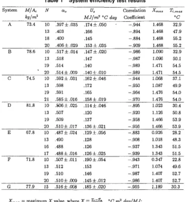
Table 1 S y s t e m efficiency test results
0.6 ^ 0 . 5 -£ O.A-cu £ 0.3 UJ 0.2 (b) System B <*„= 0.51A U s = 0.140 MJ/m2°C day I '1 1 i n U N i | i i i | i i i | u i | i i i | i i i | i U | i i i | -0.6 -O.A -0.2 0.0 0.2 0.4 0.6 0.8 1.0 1.2 1.4 1.6 0.7 ^ 0 . 6 £ 0.5 Q J £ 0.4 ijj 0.3 (c) System C rt„ = 0.585 U s = 0.1 58 M j / m ' T d a y I i I 11 I i | I i 11 i I I | i i i 11 i 11 11 11 11 111 i I 11 i i 11 i i | 6 . 6 - 0 . 4 - 0 . 2 0.0 0.2 0.4 0.6 0.8 1.0 1.2 1.4 1.6 0.6 ^ 0 . 5 £ 0.4
i
°-H
LU 0.2 (d) System D d0= 0.510 Us = 0.136 MJ/m2"C day . M 11 i i | i i i | i n | i 11 11 M | 11 i | l i i | 11 i 11 i i | i i i 0.6 0.4 0.2 0.0 0.2 O.A 0.6 0.8 1.0 1.2 1.4 1.6 X,m2°C day/MJFig. 1 Efficiency test results (System A to S y s t e m D)
0.6 f="0.5 £ 0 . 4 -OJ § 0 3 UJ 0.2 (e) System E « „ = 0.488 U s = 0.126 MJ/m2°C day - 0 , 0.7 £ 0 . 6 >. 0.5 u I 0.4 -u ip 0.3 0.2 0.7 ( ? 0 . 6 >. 0.5 S 0.4 r 0.3 UJ 0.2 i 11 I i i M i i I I 11 111 i I 11 111 11 i I I I i | i i i | I i I 11 11 | . 6 - 0 . 4 - 0 . 2 0.0 0.2 0.4 0.6 0.8 1.0 1.2 1.4 1.6 (f) System F ao= 0.510 U s = 0.14 5 MJ/m'C day I 111 11 i I i i i | i i i | i 11 11 i 11 1111 11 11 11 i11 i i | i 11 | 0 . 6 - 0 . 4 - 0 . 2 0.0 0.2 0.4 0.6 0.8 1.0 1.2 1.4 1.6 (g) System G « „ = 0.516 U s = 0.185 M j / m2* C day I i i 11 i i i I i i i I I I i 1 1 1 1 1 1 i i I 1 1 11 i ' i I i i i I i I i I -0.6 - 0 . 4 - 0 . 2 0.0 0.2 O.A 0.6 0.8 1.0 1.2 1.4 1.6 X,m2 0C d a y / M J
Fig. 2 Efficiency test results (System E to S y s t e m G)
5 System Efficiency Test Results
5.1 Testing Conditions. It is found in the present study that the operating conditions for the daily efficiency test of solar thermosyphon water heaters can be defined as follows:
System A B C D E F G M/A kg/m2 73.4 78.6 74.5 81.8 67.8 71.8 77.9 N 10 13 18 20 10 13 19 20 10 13 19 21 10 13 19 20 10 13 16 17 10 13 19 20 15 Q „ .397 ± . 0 3 5 .403 .400 .406 ± . 0 2 9 .517 ± . 0 1 4 .518 .514 .514 ± . 0 0 9 .592 ± . 0 3 1 .598 .591 .585 ± . 0 1 6 .506 ± . 0 2 5 .507 .509 .510±.017 .487 ± . 0 2 4 .490 .488 .488 ± . 0 1 6 .507 ± . 0 1 1 .512 .510 .510 ± . 0 0 9 .516 ± . 0 0 8 u, MJ/m2 °C day .174 ± . 0 5 0 .166 .145 .153 ± . 0 3 5 .147 ± . 0 2 0 .147 .140 .140 ± . 0 1 0 .162 ± . 0 4 6 .172 .165 .158 ± . 0 1 9 .114 ± . 0 4 6 .120 .137 .136 ± . 0 2 1 .129 ± . 0 5 6 .128 .126 .126 ± . 0 2 5 .190 ± . 0 5 4 .153 .146 .145 ± . 0 1 2 .185 ± . 0 2 0 Correlation Coefficient -.944 - . 8 9 4 - . 8 8 4 - . 9 0 9 - . 9 8 6 - . 9 8 7 -.989 -.989 -.944 -.950 -.964 - . 9 7 0 - . 8 9 5 - . 9 2 0 - . 9 5 8 -.956 -.883 -.908 - . 9 3 7 - . 9 3 9 - . 9 4 3 - . 9 7 1 -.987 - . 9 8 6 - . 9 5 5 Xma, 1.468 1.468 1.468 1.468 1.090 1.096 1.471 1.471 1.068 1.087 1.476 1.476 1.023 1.126 1.466 1.466 0.926 1.018 1.343 1.343 0.347 1.074 1.407 1.407 1.189 Ti,max °C 32.9 47.9 55.2 55.2 32.9 50.1 54.5 54.5 37.1 49.9 54.0 54.0 30.4 50.8 53.9 53.9 28.2 48.3 51.5 51.5 22.8 49.6 52.7 52.7 30.3
- maximum X value, where X = '• °C m2 day/MJ; Ti>max — maximum initial tank temperature.
(1) period of " d a y " for the energy collecting phase: nine hours with symmetry to the solar noon time,
(2) accumulated irradiation incident upon the collector slope H, > 7 MJ/m2 day for each test day,
(3) daily-mean wind speed v„ < 3 m/s for each test day, (4) the operating variable X = (7} - Ta)/H, satisfies
-0.5 < X < 2°C m2 day/MJ, and
(5) at least ten test points which satisfy the above conditions have to be taken, i.e., to run the test for at least ten available days.
It can be shown from Eq. (5) that the proportionality con-stant Ut is function of the period of " d a y " (At = tf - /,) and
so is Us ( = U,/Ac). From Eq. (13), a0 is function of At as well. Therefore, seasonal variation of a0 and Us is expected if At is not fixed. The period of " d a y " (At) is chosen as a fixed nine hours for all the tests in order to avoid the seasonal variation on a0 and Us. The nine hours of the daily test period
is chosen long enough such that it is closer to the daily operating hours in practical applications. Thus, the test results can also reflect the real performance.
5.2 Model Verification. Seven commercial solar ther-mosyphon systems (A, B, C, D, E, F, G) were tested in the present study. System A through F are tested simultaneously by the expert system; while System G was separately tested earlier by another testing equipment. Test results of daily ef-ficiencies are shown in Figs. 1 and 2. It can be seen that the system efficiency model, Eq. (12), can fit the test results very well indeed. It can be seen from Table 1 that the absolute values of the correlation coefficients for all the systems tested with N = ten days are > 0.88. Hence, this can validate the system efficiency model, Eq. (12). The 95 percent confidence intervals of the system parameters a0, Us (shown as the " ± "
sign) are also presented in Table 1 in which .A^x represents the maximum X value of the testing conditions, where
X= T,-Ta
H, ' (17)
7;,max is the maximum initial tank temperature in the tests.
It is further shown in Table 1 that higher correlation can be obtained as the number of available test days Ware larger than ten. The absolute values of the correlation coefficients are getting closer to 1.0 (> 0.95 for all systems except System A and E) and the 95 percent confidence intervals of ao and Us become smaller as TV increases.
0.7-t (?0.6^ u °'5~ £ 0.4-u 0.3-UJ 0.2 (a) System H <K„= 0.512 Us= 0.144 MJ/m2°C day I I | I I I | I I I | I I I | I I I | M I | I I I | I I I | I I I | I I I | I I 11 -0.6-0.4-0.2 0.0 0.2 0.4 0.6 0.8 1.0 1.2 1.4 1.6 0.7( ? 0 . 6 £ 0 . 5 £ 0 . 4 -E 0.3 UJ 0.2 (b) System H a0 = 0.514 Us = 0.156 MJ/m'°C day i 11 i l | i i i | i i i j i i i | i i i | 11 i | 11 11 1 1 1 11 i i | i i i | -0.6 -0.4 -0.2 0.0 0.2 0.4 0.6 0.8 1.0 1.2 1.4 1.6 X,m2oC day/MJ
Fig. 3 Repeatability test results for System H; (a) test period: 5/7/1990 to 5/28/1990; (b) test period: 9/15/1990 to 10/12/1990
Table 2 Effect of wind speed on system efficiency System A C D E Date 0223 0227 0206 0220 0216 0227 0219 0221 0216 0206 X .5101 .5046 .4602 .4713 .6725 .6848 1.0230 .9954 .3116 .3032 1, % 31.56 35.78 28.75 34.68 52.34 47.48 35.63 38.60 46.54 42.07 vw m/s 2.59 1.76 2.13 1.75 .68 1.76 2.48 .80 .68 2.13 ««.,.J mjs 1.38 1.06 1.05 1.48 .65 1.06 1.32 .84 .65 1.05 H, MJ/m2 13.733 20.536 15.289 14.800 8.036 20.536 11.980 8.671 8.036 15.289 % °C 27.30 33.30 26.00 28.40 27.30 37.00 30.40 28.80 24.40 23.60 T, 'C 41.40 57.20 40.30 45.10 40.80 68.30 42.90 38.60 37.60 46.30 fa °C 20.29 22.94 18.96 21.42 21.90 22.94 18.14 20.17 21.90 18.96 Date = Test date in 1989
rjt = Daily efficiency, T,
fa
- Initial temperature, °C
- Daily-mean ambient temperature, °C t
a = Standard deviation of wind speed, m/s
X= {Ti - Ta)/Hu "C m2 day/MJ Ht = Daily irradiation, MJ/m2day Tj — Final temperature, "C
- Daily-mean wind speed, m/s
5.3 Test Repeatability. Repeatability is another necessary
condition to validate the system efficiency model. A System H is selected to test the repeatability. The outdoor daily ef-ficiency test was performed twice in different seasons. The results are shown in Fig. 3. The a0 values of the two tests are almost identical. But the values of U„ differ by 8.3 percent. This is due to the data scattering caused by the instantaneous random variation of irradiation, wind speed/direction, and ambient temperature. (These factors will be discussed in next section.) However, it can be shown statistically that there is no significant difference between these two values of Us, at 5 percent risk (See Appendix A).
5.4 Discussions.
5.4.1 Causes of Data Scattering. Although the correla-tion coefficients in fitting the test data to the model, Eq. (12), are quite close to - 1.0, slight scattering still exists, especially for System A, C, D, and E. The scattering results mainly from vapor blockage in the flow passage. It was found from a field inspection that the riser pipe of System A has an improper vertical curvature so that vapor bubble was trapped there and affected the loop resistance. Trap of vapor bubbles was also found in the header tube of the collectors in System A, C, D, and E due to parallel connection of the collectors with only one outlet on the top of the collectors. Thus, trap of vapor bubbles in the collector took place easily during the tests and increases the loop resistance, and hence causes the daily system efficiency to decrease (Huang, 1981; Huang, 1989). The quan-tity of trapped vapor bubbles may vary with solar irradiation. For a variable weather condition, the occurrence of vapor bubble trap thus behaves random and causes to the scattering of the final test results. To reduce this kind of scattering, it is necessary to install the collectors and the connecting pipes carefully such that vapor bubbles will not be trapped in the flow path. In the present study, the piping and collector designs of System B, F, and G are excellent in this sense and the scattering of the test results was found very small indeed.
The other factor causing data scattering is the variation of wind speed/direction during the test. In outdoor testing, wind speed and direction changes all the time and can affect the collector performance (Green, 1988). Table 2 shows that the daily system efficiency decreases with the average wind speed for an X value approximately fixed. Since it is very difficult to control the wind speed and direction in an outdoor test, no attempt was made to reduce this effect. But, it is chosen to reject the test data if the average wind speed in each test day is higher than an allowable value, e.g., 3 m/s in the present
1 0 0 0
600
H i g h - F r e q u e n c y -f L o w - P a s s e d P a r t s
Time of Day, h r
study. On the other hand, reserving the scattering will be closer to the real situation in field applications.
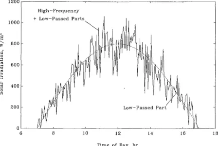
The other possible factor which may result in data scattering is the variation of solar irradiation. Instantaneous solar irra-diation usually varies all the time during the test as shown in Fig. 4. The variation of solar irradiation can approach a sine wave form with a fundamental frequency only in a very few days substantially free of clouds. The collector output tem-perature will not respond to the high-frequency part of the solar irradiation since solar collector usually has a low-pass property with time constant in the order of several minutes (Huang and Hsieh, 1991). However, the low-passed solar ir-radiation may still consist of some low-harmonics components which varies day by day and can affect the collector output temperature as well as the daily system efficiency. Therefore, the system performance over a finite number of test days will induce a data scattering along the system efficiency model. It is found in the present study and from a computer simulation (Huang, 1989) that this type of scattering is minimal if the number of test days is large enough.
5.4.2 System Performance Evaluation. Once the param-eters a0 and Us are determined, the system performance during energy collecting phase can be rated according to these two values. The system with larger a0 and smaller Us performs better, as the Case 1 in Fig. 5, with high efficiencies in the whole X range. On the contrary, the system with smaller ao and larger Us performs worse, as the Case 2 in Fig. 5, with low efficiencies in the whole X range. Another two cases are also shown in Fig. 5. Case 3 has both large a0 and Us values,
thus the efficiencies drop quickly with increasing X due to the large slope (i.e., large Us value). But the performance of the system is still good in the range of small X (i.e., lower initial temperature 7}). Case 4 has both small a0 and Us values, and thus the efficiency drops slowly with increasing X. Therefore, the system performance is poor in the range of small X, but will perform better in the range of high X (i.e., higher 7}).
Since most of the hot water collected by the thermosyphon system will be used up during the night and the make-up cold water will be fed into the tank again, the initial temperature T, is usually not very high in normal operation. Therefore, the system will be operated mostly in the range of low X values and the performance of the four thermosyphon systems shown in Fig. 5 will be rated as Case 1 > Case 3 > Case 4 > Case 2.
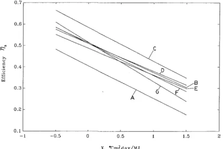
The results of the seven commercial solar systems tested in the present study are shown in Fig. 6. From the above rating criterion, the performance of System C can be rated the best in the energy collecting phase. However, it has been pointed out that the overall performance of a solar thermosyphon system cannot be rated simply from the system efficiency test. The rating must include system cooling loss test.
6 System Cooling Loss Test and Overall Performance Rating
To determine the system cooling rate of solar thermosyphon systems, the outdoor test was continued for three hours im-mediately after the system efficiency test with no solar
irra-Table 3 System cooling loss test results
0 1 2 X, m2 oC d a y / M J
Fig. 5 Performance rating based on the system efficiency test results
System A B C D E F TO days 2.75 3.20 2.69 3.76 3.00 2.63 Tc days 2.46 3.32 2.33 2.61 2.81 2.69 (fo-O/r. 11.8% - 3 . 6 % 15.5% 44.1% 6.8% - 2 . 2 % [UA)0 W/°C 4.79 4.39 5.12 3.94 4.11 3.71 (UA)t W/°C 5.39 4.25 6.00 5.68 4.41 3.64
7"0 — average cooling time constant for isolated tank, day
(UA)o ~ average heat loss coefficient for isolated tank, W/°C.
X, °Cm2day/MJ
Fig. 6 Performance rating of the systems tested
diation. The initial and final mean tank temperatures, TLi and
TLf, respectively, were measured and used to fit the system
cooling model, Eq. (15), to determine the overall cooling loss coefficient (UA), and the system cooling time constant TC. TO obtain accurate results, the test data were rejected if TLi - Ta
< 20°C.
The system cooling test results are summarized in Table 3. Here, the average values for TC measured every day are used for the rating. It can be seen that System C has the shortest TC and thus has the highest cooling loss rate. Though System C was rated the best in the energy collecting phase, it cannot be rated the best in overall performance.
It has been pointed out that, in addition to the convection loss, system cooling loss may result from flow reversal. To determine whether a flow reversal phenomenon exists, outdoor heat loss test was also performed separately for the isolated tank alone, disconnected from the system. The results T0 are presented in the second column of Table 3. By comparing the cooling time constants for the connected and isolated tanks, we can find whether there is a flow reversal phenomenon. It can be seen from Table 3 that flow reversal in System D is severe.
System A and C also have a high system cooling-loss rate which is also caused by flow reversal effect. In addition, System A has the lowest system efficiency in the energy collecting phase and thus is rated the worst in the overall performance. It is very interesting to note that the inlet position of the pipe connecting the tank of System A and C are all designed with a higher elevation relative to the collector outlet. It is thus expected that the flow reversal may easily occur (Huang, 1980; Mertol, et al., 1981; Morrison, 1985). This is quite consistent with the observed high cooling loss in these thermosyphon systems.
On the other hand, System F and B can be rated to be among the best in overall performance since their cooling loss are quite small (with TC). Apparently, system cooling loss does not involve flow reversal phenomenon in System B and F. 7 Conclusions
An attempt is made in the present study to develop a method for the thermal performance test and rating of thermosyphon systems. The present development includes the derivations of a semi-empirical system efficiency model and a method of performance testing and rating, and the design of an expert test system for the outdoor testing of thermosyphon systems. It is suggested that the overall performance rating of ther-mosyphon systems must include: (1) the system efficiency test which examines the capability of energy absorption in energy collecting phase; and (2) the system cooling loss test which examines the energy loss rate in cooling phase. Seven commercial solar water heaters are tested and the final results are analyzed and reported. The system efficiency model as well as the method of testing and rating is verified by a series of tests and analyses.
The testing method developed in the present study has been used to establish a R.O.C. National Standard (CNS B7277, 1990). This testing standard has been implemented in the expert test system for the inspection of solar hot water heaters com-mercially available. The testing task has been going on for more than one year with 31 systems tested so far. No defects of the testing standard and the expert system have been ob-served.
Acknowledgment
The present study was supported by Energy Commission, Ministry of Economic Affairs, Taiwan, Republic of China, through Grants No. 782J1 and No. 792J6 and also partly supported by National Science Council of the Republic of China, Taiwan, through Grant No. NSC78-0401-E002-18.
References
Adnot, J., Bourges, B., and Kadi, L., 1988, "The input/output method for SDHWS characterisation," Advances in Solar Energy, Vol. 1, Pergamon Press, Oxford, U.K., pp. 868-873.
Beale, S. B., 1987, "Comparison of Short-Term Testing and Long-Term Monitoring of Solar Domestic Hot Water Systems," ASME JOURNAL OF SOLAR ENERGY ENGINEERING, Vol. 109, pp. 274-280.
Close, D. J., 1962, "The performance of solar water heaters with natural circulations," Solar Energy, Vol. 6, p. 33.
Chinese National Standard CNS B7277, 1990, "Method of Test for Solar Water Heaters," CNS B7277, No. 12558, Central Bureau of Standard, Taiwan.
Fanny, A. H., 1984, "An Experimental Technique for Testing Thermosyphon Solar Hot Water Systems," ASME JOURNAL OF SOLAR ENERGY ENGINEERING, Vol. 106, pp. 457-464.
Green, A. A., 1988, "Wind speed effects in solar collector testing," Advances
in Solar Energy, Vol. 1, Pergamon Press, Oxford, U.K., pp. 768-772.
Guttman, I., Wilks, L. S. S., and Hunter, J. S., 1982, Introductory
Engi-neering Statistics, 3rd ed., John Wiley and Sons, New York.
Huang, B. J., 1980, "Similarity theory of solar water heater with natural circulation," Solar Energy, Vol. 25, p. 105.
Huang, B. J., 1989, "Development of Long-Term Performance Correlation for Solar Thermosyphon Water Heater," ASME JOURNAL OF SOLAR ENERGY ENGINEERING, Vol. I l l , pp. 124-131.
Huang, B. J., and Hsieh, S. W., 1990, "An Automation of Collector Testing and Modification of ANSI/ASHRAE 93-1986 Standard," ASME JOURNAL OF SOLAR ENERGY ENGINEERING, Vol. 112, pp. 257-267.
Kubler, R., Ernst, M., and Fisch, N., 1988, "Short term test for solar domestic hot water systems—Experimental results and long term performance predic-tion," Advances in Solar Energy, Vol. 1, Pergamon Press, Oxford, U.K., pp. 732-736.
Mertol, A., Place, W., Webster, T., and Greif, R., 1981, "Detailed loop model (DLM) analysis of liquid solar thermosyphons with heat exchangers,"
Solar Energy, Vol. 27, pp. 367-386.
Morrison, G. L., and Sapsford, C. M., 1983, "Long term performance of thermosyphon solar water heaters," Solar Energy, Vol. 30, pp. 341-350.
Morrison, G. L., and Tran, H. N., 1984, "Simulation of the long term performance of thermosyphon solar water heaters," Solar Energy, Vol. 33, No. 6, pp. 515-526.
Morrison, G. L., and Tran, H. N., 1988, "Solar water heater performance evaluation," Advances in Solar Energy, Vol. 1, Pergamon Press, Oxford, U.K., pp. 753-757.
Morrison, G. L., 1985, "Reverse circulation in thermosyphon solar water heaters," Solar Energy, Vol. 36, No. 4, pp. 377-379.
A P P E N D I X
Statistical Analysis of Tests Repeatability
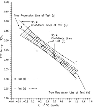
Due to the random variation of the operating conditions, the daily efficiency test results also present some kind of ran-domness. The regression analysis of the efficiency model can be further represented by the confidence bands, in addition to the regression lines presented in Figs. 1 to 3. The 95 percent confidence bands for the two regression analyses of system H are shown in Fig. Al. It can be seen that though the two parameters u0 and Us from the regression analyses for the two tests are somewhat different, the confidence bands of the two regression lines are almost overlapped. This means that it is hard to distinguish the two parameters obtained from the two tests. The repeatability of the efficiency model and the test method are thus verified.
Another way to show the repeatability of the tests is by comparing the 95 percent confidence interval of the parameters a0 and Us obtained from the linear regression analysis for the two tests. Since the regression results of a0 in Test (a) and
(b) as shown in Fig. 3 are almost identical, only Us will be
examined. The 95 percent confidence intervals of Us for the two tests are:
(a) USi„ = 0.144 ±0.038MJ/°Cm2day withsa = 0.028677
and sample size Na = 10 and
(b) UsM = 0.156 ± 0.033MJ/°Cm2day withsb = 0.022840 and sample size Nb = 11,
where Usi0 and USib are the unbiased point estimators of Us which are the linear regression results of Us from Test (a) and
(b), respectively; sa and sb are the sample standard deviation between the test points of daily efficiency and the regression
True Regression Line of Test (o) •95 %
, Confidence Lines of Test (a)
95 % Confidence Lines of Test (b)
a Test (o)
A Test (b)
True Regression Line of Test (b) i I ' i ' I i i U i ' ' I i i i I ' i i | i u | i u | u i | i i i | i u | -0.6 -0.4 -0.2 0.0 0.2 0.4 0.6 0.8 1.0 1.2 1.4 1.6
X, m!°C day/MJ
Fig. A1 Confidence bands of the regression results of System H, for Test (a) and (b)
line for Test (a) and (b), respectively. We may perform a statistical test to prove that the two point estimators USja and
0Stb are no significant difference from statistic point of view.
The test method is to calculate the t values for the two tests, where
u=-
SyfN/K' Us -fius (Al)Here, /xy is the population mean of Us, and v = N - 2 degrees-of-freedom (Guttman, Wilks, and Hunter, 1982, p. 360). The symbol A in the above equation is defined as
A
=^2>*.
-lis) (A2)where i?s,; represents the daily efficiency test points and rjs is the sample mean of ijS]/. We can calculate the t value for the two test, respectively, and then check whether these t values are acceptable. Here, we take the significance level at 5 percent. So if the calculated absolute t value, i.e., \tv\, is greater than ^,0.975. it tells that the point estimator is far away from the population mean. On the other hand, if the calculated \tv\ is smaller than ^,0.975, we can say that the point estimator is close to the population mean at 5 percent risk. We take the algebraic mean of 0St„ and USyb for the population mean JXU , i.e., fiy
= (US:a + USib)/2, thus we get
for Test (a): for Test (b): \h\ \t9\ = 0.363 < 4,0.975 = = 0.416 < ^,,0.975 = = 2.306 = 2.262
Since the two calculated 1 tv \ values are smaller than the two critical values ^,0.975, it means that the two point estimators are identical with the population mean p.us at 5 percent sig-nificant level, from statistical point of view. In other words, the two Us values obtained from the two tests shows no sig-nificant difference, at 5 percent risk. This verifies the repeat-ability of the efficiency test results again.