適應信標間距的智慧型路由器之無線隨意網路媒體存取控制協定

國 立 交 通 大 學

電信工程學系

碩 士 論 文

適應信標間距的智慧型路由器之無線隨意網路

媒體存取控制協定

Intelligent Router-Assisted Power Saving Medium

Access Control for Mobile Ad Hoc Networks with

Adaptable Beacon Intervals

研究生 : 周冠宏

指導教授 :方凱田

適應信標間距的智慧型路由器之無線隨意網路媒體存取控制協定

Intelligent Router-Assisted Power Saving Medium Access Control for

Mobile Ad Hoc Networks with Adaptable Beacon Intervals

研究生 : 周冠宏 Student : Kuan-Hong Chou

指導教授 : 方凱田 Advisor : Kai-Ten Feng

國立交通大學

電信工程學系碩士班

碩士論文

A Thesis

Submitted to Department of Communication Engineering

College of Electrical and Computer Engineering

National Chiao Tung University

in Partial Fulfillment of the Requirements

for the Degree of

Master of Science

in Communication Engineering

June 2006

適應信標間距的智慧型路由器之無線隨意網路媒體存取控制協定

學生 : 周冠宏 指導教授 : 方凱田

國立交通大學電信工程學系碩士班

摘 要

在無線隨意網路中，電池量是有限的，所以節省電池量一直是個重要

的研究議題。在一些舊有的媒體存取控制的協定裡，雖然達到了省功

率的效能，但是也浪費了頻寬，包括封包的延遲時間，傳送率等等。

那我們提出的智慧型路由器演算法，就是能預測封包經過的下一個節

點，在媒體存取控制層，我們利用一塊記憶體去紀錄擇路層的資訊，

使我們在媒體存取控制曾就可以把封包快速的送到目的地。並且我們

也發現信標間距的大小也會影響功率的消耗，IEEE 802.11 的省電機

制，信標間距是固定的，會造成頻寬的浪費，所以我們計算適應性信

標間距，計算出我們要的信標間距，不會造成頻寬的浪費，也節省功

率的消耗。在配合我們的智慧型路由器演算法，達到省功率，減少延

Intelligent Router-Assisted Power Saving Medium Access Control for

Mobile Ad Hoc Networks with Adaptable Beacon Intervals

Student : Kuan-Hong Chou Advisor : Kai-Ten Feng

Department of Communication Engineering

National Chiao Tung University

Abstract

The limitation on the battery life has been a critical issue for the

advancement of the mobile computers. Users encounter unsatisfactory

battery power while using their mobile devices, especially on the

occasions of transmitting data using the wireless networks. It has been

studied that the amount of energy consumed within the mobile devices is

significantly affected by the design of the Medium Access Control (MAC)

protocol within the wireless interface. This thesis presents a Intelligent

Router-Assisted (IRouter) power-saving MAC algorithm that achieves

energy conservation by predicting the next hopping node within the

delivering route. With the assistance of the intelligent routers in the

network, the packet delivery between several mobile nodes can be

accomplished within the same beacon interval. It has been studied that the

duration of the beacon interval is relative to the power consumption. In

this thesis, we adjust the duration of the beacon interval in the IRouter

scheme to conserve energy, and the concept of adaptable beacon interval

is presented. The performance comparison between the proposed IRouter

algorithm and the existing MAC protocols is conducted via simulations.

It is observed that the IRouter scheme can achieve feasible performance

in both energy conservation and routing efficiency.

誌 謝

千呼萬喚始出來，兩年多來所做的東西，都收錄在這本論文裡

面。首先要感謝的就是我的指導教授方凱田教授，老師提供了很多想

法及方向，讓我在茫茫的學海中，找到了燈塔並指引方向。再來就要

感謝電信的李程輝教授跟資工的趙禧綠教授，撥空來參加口試，並給

了許多寶貴的意見，並順利讓我通過口試。

接著要感謝的就是實驗室的戰友(死歐、雄光、中義、小華、阿

魯咪)，因為大家都同在屋簷下，所以更要一起努力。還要感謝這兩

年來認識的許多人(小瑩、小南、恆如、寶寶、小巫、小魚、小紫)，

在我研究所苦悶的時候，豐富了我的生活。當然還有實驗室學長跟學

弟們，也給予我ㄧ些幫助。最後要感謝的就是我的家人，家是最溫暖

的避風港，不管什麼時候家人都會給我溫暖的祝福，還會到廟裡替我

拜拜，保佑我一切順利，所以也要感謝暗中保佑我的神明。最後的最

後，也要感謝一下自己，這兩年來有苦有樂，苦的時候自己也都撐過

去了，實在是太偉大，太厲害了，不由得佩服一下自己。要感謝的人

太多了，不是短短幾個字能表達我內心的感謝，所有對我好對我關心

的人，我都非常感謝，謝謝大家，我終於不負大家期望畢業了。

周冠宏謹誌 于交通大學

Contents

1 Introduction 6

2 Key Componets and Related Work in MANET 10

2.1 MAC layer . . . 10

2.1.1 Distributed Coordination Function . . . 11

2.1.2 Hidden Node Problem . . . 12

2.1.3 Exposed Terminal Problem . . . 14

2.2 IEEE 802.11 Power-Saving Mechanism (PSM) . . . 14

2.3 Some MAC Power-Saving Protocols . . . 16

2.3.1 Asynchronous MAC Protocols . . . 17

2.3.2 Power Controlling Protocols . . . 20

2.3.3 Topology Controlling Protocols . . . 20

3 Analysis of Adaptable Beacon Intervals (ABIs) 25 3.1 IEEE 802.11’s Timing Synchronization Function . . . 25

3.2 The Analysis of Beacon Intervals (BIs) . . . 27

3.3 The Relationship between The Probability of Collision and Neighbor nodes . . 31

3.4 The Calculation of Adaptable Beacon Intervals (ABIs) . . . 33

4 The Intelligent Router-Assisted (IRouter) Power Saving Medium Access Control Algorithm 37 4.1 Assumptions and Concepts . . . 38

4.2 The IRouter Algorithm . . . 39 4.2.1 P RT Construction Process . . . 41

4.2.2 Route Prediction Process . . . 42 5 Performance Evaluation 46 5.1 Simulation Parameters . . . 46 5.2 Simulation Results . . . 47

5.2.1 Topology 1 (three fixed nodes; one source node, one router node, and one destination node) . . . 48 5.2.2 Topology 2 (six fixed nodes; two source nodes, two router nodes, and

two destination nodes) . . . 51 5.2.3 Topology 3 (random way points) . . . 51

List of Figures

1.1 (a)Ad hoc Network: Node A Communicate with Node C via Mobile Node (b)Infrastructure Network: Node A Communicate with Node C via Infrastructure 7

2.1 The Medium Access via Different Inter Frame Space (IFS) . . . 12

2.2 Hidden Node Problem . . . 13

2.3 Timing Diagram of RTS/CTS Packet Exchange . . . 13

2.4 Exposed Terminal Problem . . . 14

2.5 An Example of Network Topology . . . 15

2.6 The Timing History of Node A, B, and C . . . 16

2.7 Structures of Odd and Even Intervals in the Dominating-Awake-Interval Protocol 18 2.8 An Example of the Periodically-Fully-Awake-Interval Protocol with Fully-Awake Intervals Arrive Every p = 3 Beacon Intervals . . . 18

2.9 Examples of the Quorum-Based Protocol (a)Intersections of Two PS Nodes Quorum Intervals, (b)Node A’s Quorum Intervals, and (c)Node B’s Quorum Intervals . . . 19

2.10 The Power Control Scheme . . . 21

2.11 Differences in Transmit Power Lead to Increased Collisions . . . 21

2.12 The First ATIM Period Ending Rule . . . 23

2.13 The Second ATIM Period Ending Rule . . . 23

2.14 The Channel Capture Problem . . . 24

3.2 The MN Receives Beacon, Compares the Clock, and Modifies the Clock . . . . 26

3.3 Different Length of BI . . . 30

3.4 The Defer Mechanism in IEEE 802.11 . . . 31

3.5 The Relationship between the Probability of Collision (Pcollision) and the Num-ber of Neighbor Nodes (N ) . . . 33

3.6 Ptotal , C, and the Cost Function (cost) . . . 36

4.1 The Timing Diagram of the IRouter Scheme . . . 38

4.2 The Network Topology with the Proposed IRouter Scheme . . . 40

4.3 The IRouter MAC Scheme Will Check the P RT and PRj downhP, N i . . . 44

5.1 The Network Topology 1 (Three Fixed Nodes; One Source Node, One Router Node, and One Destination Node) . . . 48

5.2 Performance Comparison: Remaining Energy vs Data Rate . . . 49

5.3 Performance Comparison: Packet Delivery Ratio vs Data Rate . . . 49

5.4 Performance Comparison: End-to-End Delay vs Data Rate . . . 50

5.5 Performance Comparison: Control Packet Overhead vs Data Rate . . . 50

5.6 The Network Topology 2 (Six Fixed Nodes; Two Source Nodes, Two Router Nodes, and Two Destination Nodes) . . . 51

5.7 Performance Comparison: Remaining Energy vs Data Rate . . . 52

5.8 Performance Comparison: Packet Delivery Ratio vs Data Rate . . . 52

5.9 Performance Comparison: End-to-End Delay vs Data Rate . . . 53

5.10 Performance Comparison: Control Packet Overhead vs Data Rate . . . 53

5.11 The Cost Function (Numbers of Nodes = 64) . . . 54

5.12 Performance Comparison: Remaining Energy vs Velocity (Numbers of Nodes = 64) . . . 55

5.13 Performance Comparison: Packet Delivery Ratio vs Velocity (Numbers of Nodes = 64) . . . 55

5.14 Performance Comparison: End-to-End Delay vs Velocity (Numbers of Nodes = 64) . . . 56 5.15 Performance Comparison: Control Packet Overhead vs Velocity (Numbers of

Nodes = 64) . . . 56 5.16 Performance Comparison: Remaining Energy vs Number of Nodes (Velocity =

10 m/s) . . . 57 5.17 Performance Comparison: Remaining Energy vs Velocity (Numbers of Nodes

= 64) . . . 58 5.18 Performance Comparison: Packet Delivery Ratio vs Number of Nodes (Velocity

= 10 m/s) . . . 58 5.19 Performance Comparison: Packet Delivery Ratio vs Velocity (Numbers of Nodes

= 64) . . . 59 5.20 Performance Comparison: End-to-End Delay vs Number of Nodes (Velocity =

10 m/s) . . . 59 5.21 Performance Comparison: End-to-End Delay vs Velocity (Numbers of Nodes

= 64) . . . 60 5.22 Performance Comparison: Control Packet Overhead vs Number of Nodes

(Ve-locity = 10 m/s) . . . 60 5.23 Performance Comparison: Control Packet Overhead vs Velocity (Numbers of

Chapter 1

Introduction

A Mobile Ad hoc NETwork (MANET) consists of wireless Mobile Nodes (MNs) that coop-eratively communicate with each other without the existence of fixed network infrastructure. Fig. 1.1 shows the framework of wireless ad hoc network, where each MN communicates with others not via infrastructure but the peers. Depending on different geographical topologies, the MNs are dynamically located and continuously changing their locations. Recent interests in the design of MANET algorithms include applications for the military, the Inter-Vehicle Communication (IVC), the Personal Communication Services (PCS), and the sensor networks. The MANET is not only used in military communication but can also be applied generally in Inter-Vehicle Communication (IVC), message delivery, disasters recovery, sensor network, the Personal Communication Services (PCSs), and educational purpose. There are two examples of MANET described as follows:

• The Intelligent Transportation System (ITS): With the capability of self-organizing,

the MANET provides the wireless communication routes between vehicles. This capa-bility is also useful when emergencies happen in rural area because it will be much easier to communicate with police using MANET. Similarly, the MANET can help to save lives in mountains or in seas which have no expected network infrastructure provided. In the limited space and time, the MANET is especially satisfactory because of its wireless and movable features.

Figure 1.1: (a)Ad hoc Network: Node A Communicate with Node C via Mobile Node (b)Infrastructure Network: Node A Communicate with Node C via Infrastructure

• The Personal Communication Service (PCS): As the personal communication

de-vices are becoming more powerful, the related technology is required to deal with mass data transmission, including computer files exchange and exhibition of application pro-grams. The MANET can provide data transmission efficiently by forming a temporary network topology instead of a large infrastructure or a point-to-point transmission line. Since most of the MN’s are battery-powered devices, how to minimize the MN’s energy consumption becomes an important issue in the protocol design within MANETs. In the infrastructure-based networks, the MNs can be scheduled to be in the sleep state by the centralized server while they are not actively transmitting or receiving data. However, it is challenging to design a feasible power control mechanism within the decentralized and fast-changing ad hoc networks [1]. An efficient power-saving mechanism should be incorporated within the protocol design in order to conserve the MN’s energy; while the routing efficiency can still be preserved under the dynamic changing networks.

Many research studies have been carried out in the design of power-saving mechanism for MANETs. The protocol designs are considered in different network layers [2]- [12], especially in the Medium Access Control (MAC) layer and the routing layer. A feasible design of the power-saving MAC scheme will be the primary focus in this thesis.

However, most of the research studies consider their power-saving MAC schemes within a single hop between the MNs. The power level of the MN is turned to the sleep state while it is not either transmitting or receiving data packets. A large amount of the existing power-saving schemes conserve the MNs’ energy but induce worse routing efficiency, including longer end-to-end routing delay and excessive packet loss. In this thesis, an Intelligent Router-Assisted (IRouter) power-saving MAC protocol is proposed to offer efficient packet delivery with min-imal power consumption for the MANET. The proposed IRouter scheme incorporates partial routing information within the power-saving MAC protocol design. Each MN maintains a cache memory which updates the information of the predicted next hopping nodes within the delivering routes. Based on the partial routing information, multi-hop packet delivery can be achieved within a single beacon interval. The proposed IRouter scheme results in improved routing efficiency and power consumption within the MAC layer. The effectiveness of the IRouter MAC algorithm is validated via the simulation results.

Some of the research show that the duration of the beacon interval affects the power consumption. In the IEEE 802.11 PSM, the beacon interval is divided into the ATIM window and the remaining beacon interval. The duration of the ATIM window and the remaining beacon interval will also affect the power consumption. If the duration of the beacon interval is large, the power consumption will increase; while the duration of beacon interval is short, the numbers of control packets will increase. There is tradeoff between the power consumption and the numbers of control packets. We will calculate the duration of adaptable beacon interval (ABI), which allows one transmission pair. According to our presented cost function, we can determine the transmission pairs that are allowed in one beacon interval. The adaptive beacon interval scheme will be added to the IRouter algorithm to further provide efficient energy conservation.

The remainder of this thesis is organized as follows. Chapter 2 introduces the key compo-nents and related work of MANET in MAC layer. Chapter 3 shows the analysis of adaptable beacon intervals (ABIs). The proposed IRouter algorithm is presented in Chapter 4. The simulation parameters and the performance evaluation of the proposed IRouter algorithm are

Chapter 2

Key Componets and Related Work

in MANET

In this section, the key components which enable the communication in ad hoc networks will be presented.

According to the structure of Open System Interconnect (OSI), the radio propagation model are utilized to formulate the radio phenomenon and the baseband system to achieve the data transmission between MNs in the physical layer. In the MAC layer, how nodes share the same medium is an important issue in the wireless system. How to decide the routing path between the source nodes and the destination nodes is considered in network layer. In this thesis, we focus on the MAC protocols, so the MAC layer protocols will be studied in section 2.1. The IEEE 802.11 power-saving mechanism (PSM) will be described in section 2.2. Some MAC power-saving protocols will also be investigated in section 2.3.

2.1

MAC layer

In this section, the mechanisms of IEEE 802.11 Medium Access Control (MAC) are described. The MAC layer provides several services, including packets exchange, synchronization, and channel utilization. It is also responsible for interpreting the received bit stream from the physical layer to the network layer.

2.1.1 Distributed Coordination Function

The Distributed Coordination Function (DCF) is a basic access mechanism utilized by the MAC protocol in IEEE 802.11. The DCF is based on a Carrier Sense Multiple Access (CSMA) with Collision Avoidance (CA), which guarantees each station a fair chance to access the medium.

By using the CSMA/CA scheme, each node has to sense the medium before data trans-mission. If the medium is found idle, the data is allowed to be sent. In order to avoid collision, the station selects a random backoff time slots and freezes transmission until the time slot is decreased to zero. The MANET is a self-organized network without centralized node to control the usage of medium. The IEEE 802.11 DCF is a simple and fair mechanism that satisfies the requirement of MANET.

However, the fast changing characteristic of wireless medium makes the correct operation of carrier sense a difficult problem. The IEEE 802.11 MAC protocol provides additional mean called virtue carrier sensing as a backup mechanism to avoid collisions. Virtual carrier sensing is carried out by NAV (Network Allocation Vector), which records the duration of ongoing data transmission. The data can be transmitted only when both physical and virtual carrier sense mechanism detect that the medium is idle.

Before the data transmission, each station executes backoff process to ensure the low probability of collision. The station uniformly selects the time slots between the interval of [0, CW ], which is predefine by IEEE 802.11. The minimum of contention window (CW ) size is 31. The maximum of contention window (CW ) size is set to be 1023. However, the stations may choose the same time slots under congestion networks. The binary exponential backoff algorithm is executed by using double CW size to avoid the collision again.

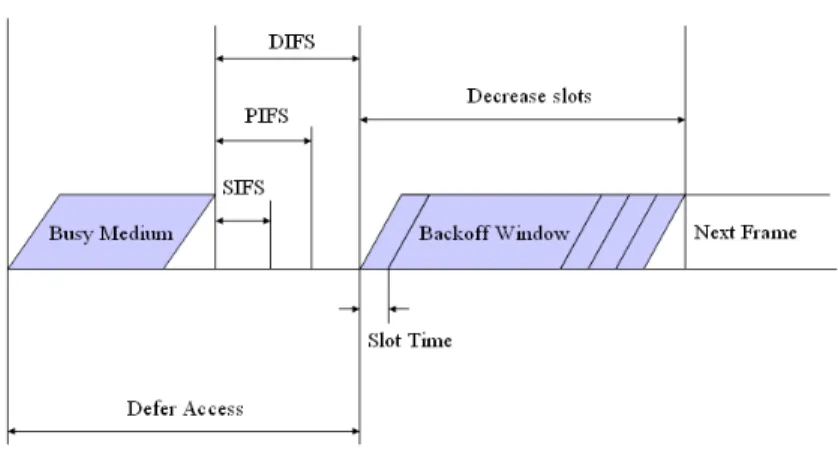
The IEEE 802.11 MAC defines multiple Inter Frame Space (IFS) which are utilized to provide different priorities for medium access including short IFS (SIFS), PCF IFS (PIFS), DCF IFS (DIFS), and Extended IFS (EIFS). As shown in Fig. 2.1, the SIFS is the shortest time spacing with which the station can immediately response the request like Ack and CTS. The Point Coordinator Function (PCF) is a contention free service and the infrastructure

Figure 2.1: The Medium Access via Different Inter Frame Space (IFS)

is responsible for monitoring the transmission between each station. To ensure the service being contention free, DIFS > PIFS can avoid the DCF interfering the transmission of PCF. Finally, waiting the largest time spacing EIFS means the packet retransmission (i.e. collision occurs).

2.1.2 Hidden Node Problem

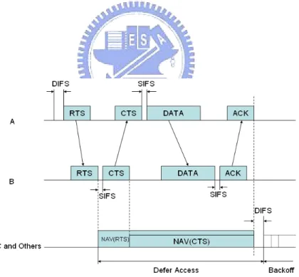
Due to the limited transmission range, the CSMA can not detect the data transmission that are out of the sensing range, which causes the hidden node problem. The hidden node problem will result in the degradation of performance. As shown in Fig. 2.2, the node A is transmitting a packet to node B. At this moment, the node C also initiates a new transmission but the carrier sense can not function since C is outside the transmission range of node A. The collision will occur at node B and node A has to retransmit the packet.

The solution of hidden node problem is that each station exchanges smaller packets called RTS and CTS to reserve the channel before data transmission. In Fig. 2.3, node A sends RTS to node B and node B replies a CTS to node A. It is noted that node C is also informed not to send packet by receiving the CTS.

Figure 2.2: Hidden Node Problem

Figure 2.4: Exposed Terminal Problem

2.1.3 Exposed Terminal Problem

The RTS/CTS mechanism protects the data by blocking the nodes around the transmission pair, which degrade the throughput of network. Fig. 2.4 shows the exposed terminal problem. Because node A is blocked by the CTS of node B, node D can not send its packet to node A even if this transmission will not affect node B and node C.

2.2

IEEE 802.11 Power-Saving Mechanism (PSM)

In ad hoc networks, battery power is an important resource since most terminals are battery powered. Terminals consume extra energy when their network interfaces are in the idle state or when they overhear packets not destined for them. They should, therefore, switch off their radio when they do not have to send or receive packets. IEEE 802.11 features a power saving mechanism (PSM) in Distributed Coordination Function (DCF). In PSM for DCF, nodes must stay awake for a fixed time, called the ATIM window (Ad-Hoc Traffic Indication Map window). If nodes do not have data to send or receive, they enter the sleep state except for the ATIM window duration. However, ad hoc networks with PSM have longer end-to-end delays to deliver packets and suffer lower throughput than the standard IEEE 802.11.

The IEEE 802.11 PSM [2] is adopted as the baseline mechanism for the proposed IRouter scheme, and the IRouter scheme will be described in chapter 4. The primary functionality

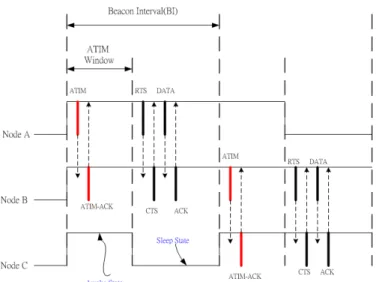
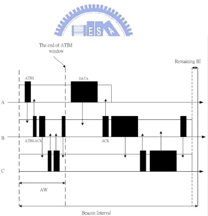
Figure 2.5: An Example of Network Topology

of the PSM is to reduce the power consumption by setting those inactive MNs into the sleep state. As illustrated in Fig. 2.5, the partial route for transmitting data from node A, via B, to C are selected by an ad hoc routing algorithm. It is noted that nodes A and C are not in the directed communication range. The timing histories of the three MNs, A, B, and C (as shown in Fig. 2.6) are divided into Beacon Intervals (BIs). The BIs are synchronized by sending beacon frames between the MNs, which also signal all the MNs to be in the awake state. The PSM defines the ATIM window starting from the beginning of each BI as shown in Fig. 2.6. As node A intends to transmit data to node B, it will send out an ATIM frame to all its neighborhood MNs after channel contention. Since the destination information (i.e. the ID of node B) is recorded within the ATIM frame, only node B will respond with an ATIM-ACK frame to acknowledge the reception of the ATIM frame. After the time for the ATIM window elapses, both nodes A and B are set to be in the awake state; while other MNs within the transmission range (i.e. nodes D, and E as in Fig. 2.5) are set to the sleep state. The data can therefore be transmitted from node A to B using either the RTS/CTS scheme or the conventional CSMA/CA mechanism. It is noted that the RTS/CTS scheme is an optional mechanism, which is primarily designed to resolve for the hidden terminal problem [2]. After the data packet has arrived in node B, the transmission from node B to

C will follow the similar process in the next BI (or any other BI afterwards depending on the

Figure 2.6: The Timing History of Node A, B, and C

2.3

Some MAC Power-Saving Protocols

In this section, some MAC power-saving protocols will be described. It has been observed in [3] that many power-saving schemes are based on the PSM to further improve the energy consumption under different circumstances. The study in [4] shows that the length of the ATIM window within the PSM significantly affects the routing performance. It is noted that the ATIM window is defined as the time interval for determining the MNs to be in the awake state for data transmission. The scheme in [5] modifies the 802.11 PSM by adjusting the length of the ATIM window based on the levels of network congestion. The Power Save Distributed Contention Control (PS-DCC) [6] determines its power-saving strategy by controlling the accesses to the shared transmission channel. The PAMAS protocol [7] utilizes busy tones in a separate signaling channel to control the packet transmission in the data channel. In additions, several routing layer schemes for power-saving purpose are proposed in [8] [9] [10] [11]; while [12] presents a cross-layer power management system for the MANET. Power can be saved during the clustering stage [13] [14], and also by reducing contention in the MAC layer [15] [16]. Also research has been done based on IEEE 802.11s power management scheme, which puts idle stations (those with no traf- fic coming in or out) into sleep by shutting down their transceivers [17] [18] [19]. We will describe three representative MAC protocols; one is

asynchronous protocol; another is power controlling protocol; the other is topology controlling protocol.

2.3.1 Asynchronous MAC Protocols

Many MAC protocols are synchronous. In [20] there are three asynchronous power-saving protocols based on the IEEE 802.11 PS mode.

• Dominating-awake-interval protocol: The basic idea of this approach is to impose

a PS node to stay awake sufficiently long so as to ensure that neighboring nodes can know each other. A PS node should stay awake for at least about half of BI in each beacon interval in dominating-awake-interval protocol. The sequence of beacon intervals is alternatively labeled as odd and even intervals. Odd and even intervals have different structures as defined below (see the illustration in Fig. 2.7). Each odd beacon interval starts with an active window. The active window is led by a beacon window and followed by an MTIM window. The function of MTIM window is like ATIM window. Each even beacon interval also starts with an active window, but the active window is terminated by an MTIM window followed by a beacon window. The above theory guarantees that a PS node is able to receive all its neighbors beacon frames in every two beacon intervals, if there is no collision in receiving the latters beacons. Since the response time for neighbor discovery is pretty short, this protocol is suitable for highly mobile environments. But, the power consumption is very large.

• Periodically-fully-awake-interval protocol: two types of beacon intervals are

de-signed in this protocol to reduce the active time: low-power intervals and fully-awake intervals . Low-power intervals and fully-awake intervals have different structures as defined below (see the illustration in Fig. 2.8). Each low-power interval starts with an active window, which contains a beacon window followed by an MTIM window, such that Active Window(AW) = Beacon Window(BW) + MTIM Window(MW). In the rest of the time, the node can go to the sleep mode. Each fully-awake interval also starts with a beacon window followed by an MTIM window. However, the node must remain

Figure 2.7: Structures of Odd and Even Intervals in the Dominating-Awake-Interval Protocol

Figure 2.8: An Example of the Periodically-Fully-Awake-Interval Protocol with Fully-Awake Intervals Arrive Every p = 3 Beacon Intervals

awake in the rest of the time, i.e., AW = BI. The beacon intervals are classified as low-power and fully-awake intervals. The fully-awake intervals arrive periodically every p intervals, and the rest of the intervals are low-power intervals. If p is bigger, the power is more efficient.

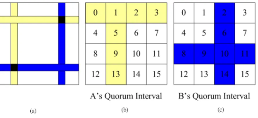
• Quorum-based protocol: In this protocol, a PS node does not need to send beacons

in every beacon interval. The sequence of beacon intervals is divided into sets starting from the first interval such that each continuous n2 _{beacon intervals are called a group,}

where n is a global parameter. In each group, the n2 _{intervals are arranged as a}

2-dimensional n × n array in a row-major manner. On the n × n array, a node can arbitrarily pick one column and one row of entries and these 2n − 1 intervals are called

Figure 2.9: Examples of the Quorum-Based Protocol (a)Intersections of Two PS Nodes Quo-rum Intervals, (b)Node A’s QuoQuo-rum Intervals, and (c)Node B’s QuoQuo-rum Intervals

quorum intervals. The remaining n2− 2n + 1 intervals are called non-quorum intervals.

The structures of quorum and non-quorum intervals are formally defined below. Each quorum interval starts with a beacon window followed by an MTIM window. The node must remain awake for the rest of the interval, i.e., AW = BI. Each non-quorum interval starts with an MTIM window. After that, the node may go to the sleep mode, i.e., we let AW = MW. This is due to the fact that a column and a row in a matrix always have an intersection (see the illustration in Fig. 2.9(a)). Thus, two PS nodes may hear each other on the intersecting intervals. For example, in Fig. 2.9(b) and (c), node A selects intervals on row 0 and column 1 as its quorum intervals from a 4 × 4 matrix, while node B selects intervals on row 2 and column 2 as its quorum intervals. When perfectly synchronized, intervals 2 and 9 are the intersections.

Above three asynchronous MAC protocols are suitable for different environments. Dominating-awake-interval protocol is suitable for highly mobile environment but doesnt conserve energy since it requires PS node to keep active more than half of the BI. Periodically-fully-awake-interval protocol can save more power as long as p > 2 and is more appropriate for slowly mobile environments. Quorum-based protocol only need to send beacons in some BIs. The periodically-fully-awake-interval and the quorum-based protocols active ratios can be quite small as long as p and n, respectively are large enough. The Dominated-Awake-Interval

proto-col is most sensitive to neighbor changes, while the Quorum-based protoproto-col is least sensitive.

2.3.2 Power Controlling Protocols

Most MAC protocols are synchronous, and there are usually two broad ways to achieving less energy consumption. One is topology controlling, and another is power controlling. For example, The IEEE 802.11 PSM [2] is topology controlling protocol. The power controlling protocol is changing transmission power with packets.

The algorithm in [21] [22] determines different transmission and sensing ranges to optimize the transmission energy of the MNs.The algorithm belongs power controlling protocol. The node uses maximum power level to transmit RTS and CTS packets as illustrated in Fig. 3.5. Then, the node calculate transmission power, which source node can transmit destination node suitably. Next, the node will transmit data packets with the calculated transmission power level. Because of lower transmitting power, the power consumption will decrease. The power controlling protocol also causes serious hidden node problem. As illustrated in Fig. 2.11, the transmission between node A and B will collide because of the transmission of node C and D. So, many protocols based on the idea of power controlling are developed. The study in [23] shows that the mobile nodes calculate the packet delivery cure, and modify transmission power. It shows that modes use adaptive power based on packet delivery curve. It is shown that CAPC [23] achieves similar throughput and higher throughput/energy consumption ratio than IEEE802.11 MAC protocol.

2.3.3 Topology Controlling Protocols

There are many topology controlling protocols. These protocols are usually based on the IEEE 802.11 PSM [2]. The algorithm in [24] has two functions. One is scheduling, and the other is dynamically adjusting the ATIM window size. The scheduling is proposed to avoid PS nodes contending medium again after the ATIM window without any extra overhead. Adjusting the ATIM window size dynamically is accommodating to various traffic conditions for improving network throughput and reducing PS nodes’ power consumption. The proposed protocol

Figure 2.10: The Power Control Scheme

in [24] has two main contributions. First, it avoids unnecessary frame collisions and backoff waiting time in data frame transmissions. Second, it conserve more power of PS nodes and improve to the channel utilization, and develop a intelligent strategy to dynamically shorten the ATIM window size. It is clear that reducing nodes backoff idle time and avoiding frame collisions can improve energy efficiency and network throughput. In this protocol [24] define that a buffered data frames duration, called working duration, is piggy-backed in an ATIM frame. To minimize average waiting time, it follow shortest job first policy basically, so the node with the shortest total working duration have the highest priority to transmit its buffering frames. The total working duration of a node is the sum of the working durations of all ATIM frames related it. The protocol [24] has special mechanism, which allows a PS node can go back to sleep when it completes all its data transmissions. Each node constructs the transmission table by the information in ATIM frames. Next, the nodes determine the transmission order. This is the scheduling transmission mechanism in the protocol [24]. There is no bound for the ATIM window size at the beginning of the beacon interval, and the end of the ATIM window depends on the traffic load of ATIM frames. Each node can obtain the duration of frame transmissions by overhearing ATIM frames, and calculate the total duration of all its currently receiving ATIM frames. If nodes sense the channel is idle more than T_{DIF S} + T_{CW min} , it deem that there will be no other node wanting to send ATIM frames. The ATIM window ends as illustrated in Fig. 2.12. If there is no any frame can be transmitted in the rest BI, all nodes end the current ATIM window immediately and enter the scheduled transmission as illustrated in Fig. 2.13.

Increasing spatial reuse is also a good way to reduce the energy consumption. As illustrated in Fig. 2.14, stations within the transmission range of A are all blocked due to the use of CSMA/CA mechanism when A is transmitting data to B with fixed power level. When A adjusts (decreases) its transmission power, some stations which is blocked by A will be released. Thus, C and D can transmit simultaneously when A is transmitting to B. Increasing spatial reuse is not only reducing power consumption but also increase the channel capture.

Figure 2.12: The First ATIM Period Ending Rule

Figure 2.14: The Channel Capture Problem

the ATIM window size changes, the Beacon intervals should change. In this thesis, the analysis of beacon intervals will be discussed in next chapter.

Chapter 3

Analysis of Adaptable Beacon

Intervals (ABIs)

Similar to the IEEE 802.11 PSM, synchronization between the MNs are assumed in this thesis. The synchronization signals can be obtained from a centralized control unit (e.g. Global Positioning System (GPS), Base Station, or Access Point (AP)) or a decentralized synchronization mechanism (e.g. mobile point coordinator). As shown in Fig. 3.1, the beacon packets are transmitted between the MNs at the beginning of each BI for synchronization purpose. The time interval for each BI (i.e. TBI) is generally a pre-determined parameter in

most of the wireless standards (e.g. T_BI = 0.1 ms for IEEE 802.11 PSM [2]). It can be more efficient to have adjustable T_BI based on certain network characteristics.

The concept of the Adaptable Beacon Interval (ABI) is to acquire feasible value of the ABI in order to effectively maintain system throughput and to reduce energy consumption. The following calculation and analysis are utilize to determine the reasonable value of Tbi.

3.1

IEEE 802.11’s Timing Synchronization Function

Before calculating the adaptable beacon interval, we should know the relationship between beacon frames and IEEE 802.11’s timing synchronization function. In the IEEE 802.11 PSM [2], MNs are required to be synchronous. In this section, IEEE 802.11’s timing synchronization

Figure 3.1: Nodes Send Beacons at the Beginning of BI

Figure 3.2: The MN Receives Beacon, Compares the Clock, and Modifies the Clock function will be described.

In the IEEE 802.11 PSM, the time history is divided into beacon intervals, and each beacon interval contains a beacon generation window. Each MN waits for a random number of slots to transmit the beacon frame. Beacon frames are broadcast, which contain time-stamps. On receiving a beacon, the MN will adopts beacons timing only if T(beacon) > T(MN) as shown in Fig. 3.2. So we can see that clocks only move forward, and faster clocks synchronize slower clocks. On the other hand, the time-stamps associated within the beacon frame will not be utilized if it is smaller than the time-stamps of the receiving MN.

3.2

The Analysis of Beacon Intervals (BIs)

A beacon interval consists of a beacon window (BW), an ATIM window, and the remaining BI. In the beacon window, beacon frames will be transmitted. The beacon window only takes several time slots in a beacon interval. While analyzing BIs, the beacon window can always be ignored. In the ATIM window, the ATIM frames and the ATIM-ACK frames will be transmitted. If MNs transmit or receive ATIM frames, they will be awake after ATIM window. On the other hand, if MNs do not transmit or receive ATIM frames, they will be sleep after the ATIM window to save energy. When receiving ATIM frames, MNs reply with ATIM-ACK frames. In the remaining BI, the RTS, CTS, data, and ACK frames will be transmitted.

Before analyzing the BIs, the following parameters are defined :

• tAT IM: the transmission time of an ATIM frame

• tAT IM −ACK: the transmission time of an ATIM-ACK frame

• t_{RT S}: the transmission time of a RTS frame

• tCT S: the transmission time of a CTS frame

• tDAT A: the transmission time of a data frame

• t_ACK: the transmission time of an ACK frame

• tB: the backoff time of transmitting packets

• tcollision−A: the waste time when ATIM frames collide or fail

• t_{collision−D}: the waste time when RTS frames collide or fail

• tAT IM −timeout: the timeout if ATIM frame is transmitted

• tRT S−timeout: the timeout if RTS frame is transmitted

• t_{DIF S}: the defer time of DIFS

• TAW: the duration of the ATIM window

• TRBI: the duration of the remaining BI

• TABI: the duration of Adaptable Beacon Interval (ABI)

• T_BI: the duration of a BI

• TA: the time of one transmission pair including the ATIM and ATIM-ACK frames

• TD: the time of one transmission pair including the RTS, CTS, data, and ACK frames

• P_collision: the probability of collision

In the IEEE 802.11 PSM [2], the beacon interval consists of the ATIM window and the remaining BI as :

TBI = TAW + TRBI (3.1)

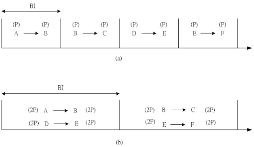
If we want to conserve more energy, a data frame should be transmitted in a beacon interval. It means that only an ATIM frame and an ATIM-ACK frame will be transmitted in a ATIM window. Certainly, a RTS, a CTS, a data, and an ACK frame will be transmitted in the remaining BI. As shown in Fig. 3.3 (a) and (b), the length of BI is different. The length in Fig. 3.3 (b) is twice as long as the length in Fig. 3.3 (a). In Fig. 3.3, node A transmits data packets to node C via node B, and node D transmits data packets to node

F via node E. It allows that only a transmission pair including an ATIM, an ATIM-ACK, a

RTS, a CTS , a data, and an ACK frame in Fig. 3.3 (a) because the length of BI is limited. For example as in Fig. 3.3 (a), node A transmits the packet to node B in the first BI. In Fig. 3.3 (b), two transmission pairs can be allowed in one BI. Node A transmits the packet to node B, and node D transmits the packet to node E in the same BI. We assume that the power consumption for one node in one BI as in Fig. 3.3 (a) is P . So we know that the power consumption for one node in one BI in Fig. 3.3 (b) is 2P because the length of BI is twice.

The total power consumption is 8P in Fig. 3.3 (a), and the total power consumption is 16P in Fig. 3.3 (b). The power consumption is less if there is only one transmission pair in one beacon interval.

We define the power in one BI which allows one transmission pair is PBI1. If the BI allows

n transmission pairs, the power consumption is nPBI1. We can get the difference of power

consumption (∆P ) in n BI :

∆P = 2n2P_BI1− 2nP_BI1 (3.2) Although the duration of one BI is reduced for energy conservation purpose, the control packets are increased. In the beginning of BI, the beacons will be transmitted. We assume that T_beacon is the duration of beacon window. The numbers of control packets (∆C) will increase, and may cause some delay time (∆T_c):

∆C = n2− n (3.3) ∆Tc= (N − 1)Tbeacon (3.4)

The minimum time interval for TAW and TRBI to transmit n successful pairs of data can

be represented as :

TAW = nTA+ Tbeacon (3.5)

TRBI = n · TD+ δ (3.6)

The δ is a modifying parameter. Because of different conditions, the δ will be different. In this thesis, the δ is ignored.

In IEEE 802.11, the numbers of transmission pairs (n) is calculated as :

n = TBI− TAW TD =

TAW− Tbeacon

Figure 3.3: Different Length of BI

The accurate length of BI for one transmission pair is hard to calculated because of the random backoff and the happening of collision. We can calculate the mean of collision time (E[t_{collision−A}], E[t_{collision−D}]) and the mean backoff time (E[tB]) to obtain the length of BI

for one transmission pair.

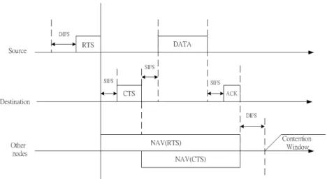
As illustrated in Fig. 3.4, we can obtain the length of TD is :

T_D = E[t_B] + t_{DIF S}+ t_{RT S}+ t_{SIF S} + t_{CT S}+ t_{SIF S}+

tDAT A+ tSIF S+ tACK+ tDIF S+ E[tcollision−D] (3.8)

The same as RTS and CTS packets exchange, so the length of T_Ais :

TA= E[tB] + tDIF S+ tAT IM + tSIF S+ tAT IM −ACK+ tDIF S+ E[tcollision−A] (3.9)

For power-saving purpose, the T_AW should be equal to T_A, and the T_RBI should be equal to TD.

TAW = TA (3.10)

TRBI = TD (3.11)

Figure 3.4: The Defer Mechanism in IEEE 802.11

3.3

The Relationship between The Probability of Collision and

Neighbor nodes

In this section, we have to calculate the mean of collision time. First, the probability of collision should be found. According to [25], it proposes that there are two kinds of the probability of collision. One is that the probability P1 for multiple nodes to transmit RTS

packets during the same time slot :

P1= ∞ X i=2 [1 − (1 − p0)i− ip0(i−1)]M i i! e −M = 1 − (1 + M p0)e−p0M (3.13) , where M is the mean number of nodes that belong to the shared channel, and p0 _{is the}

probability that a node transmits in a time slot.

The other is that the probability P2 for one node around the channel to initiate a failed

to the collision of the sending nodes RTS packet with other packets : P2 = 1 − e−p 0_M − psM e−p 0_M − (1 − (1 + M p0)e−p0M) = (p0− ps)M e−p 0_M (3.14) , where psis the probability that a node begins a successful four-way handshake at each slot.

The two equations have some unknown parameters. In [25], the mean number of nodes that belong to the shared channel is M = λπR02_{= α}2_{N where N = λπR}2_{. N is the average}

number of nodes within a circular region of radius R. It obtain R0 _{= αR where 0.5 ≤ α ≤ 2,}

and α need to be estimated. In this thesis, we assume α = 1. The throughput is relative to the different p0_{, and p}0 _{is also relative to the data arrival rate from upper layer down to}

MAC layer. According to his simulation, we assume p0 _{= 0.1 in order to get good throughput.}

The parameter ps denotes the probability that a node begins a successful four-way handshake

at each slot. In [25], a equation is used to calculate the parameter ps, but the equation is

complex. We can find that p0 is the probability which a node transmits in a time slot, and the ps is less than p0. So we assume that ps = 0.05 , the half of p0. The total probability of

collision P_collision becomes :

Pcollision= P1+ P2= 1 − (1 + M p0)e−p 0_M + (p0− ps)M e−p 0_M = 1 − e−p0N− psN e−p 0_N = 1 − e−0.1N− 0.05N e−0.1N (3.15) The probability of collision will be simplified, and it is relative to the number of neighbor nodes. As illustrated in Fig. 3.5, x-axis is the number of neighbor nodes (N ), and y-axis is the probability of collision (Pcollision).

0 5 10 15 20 25 30 0 0.1 0.2 0.3 0.4 0.5 0.6 0.7 0.8 0.9

Number of Neighbor Nodes

Probability of Collision

Figure 3.5: The Relationship between the Probability of Collision (P_collision) and the Number of Neighbor Nodes (N )

3.4

The Calculation of Adaptable Beacon Intervals (ABIs)

In this section, we can calculate the beacon interval, which is adaptable to the number of neigh-bor nodes. As mentioned in (3.8) and (3.9), we will describe how to calculate E[tcollision−D]

and E[tcollision−A]. In the IEEE 802.11, the ATIM frame can be retransmitted three times if

it fails. So the mean value of collision time of an ATIM frame is :

E[t_{collision−A}] = P_collision(E[tB] + tAT IM −timeout+ tAT IM)

+P_collision2 (2E[tB] + tAT IM −timeout+ tAT IM)

And the RTS frame can be retransmitted seven times if it fails. So the mean value of collision time of a RTS frame is :

E[tcollision−D] = Pcollision(E[tB] + tRT S−timeout+ tRT S)

+P_collision2 (2E[tB] + tRT S−timeout+ tRT S)

+P_collision3 (4E[t_B] + t_{RT S−timeout}+ t_{RT S})

+P_collision4 (8E[tB] + tRT S−timeout+ tRT S) (3.17)

+P_collision5 (16E[tB] + tRT S−timeout+ tRT S)

+P_collision6 (16E[tB] + tRT S−timeout+ tRT S)

+P_collision7 (16E[tB] + tRT S−timeout+ tRT S)

In this thesis, our adaptable beacon intervals (ABIs) is different according to the number of neighbor nodes. Above all, We conclude that the duration of ABIs is :

TABI = TAW + TRBI = TA+ TD = E[tB] + tDIF S+ tAT IM

+tSIF S+ tAT IM −ACK+ tDIF S+ E[tcollision−A]

+E[t_B] + t_{DIF S}+ t_{RT S}+ t_{SIF S}+ t_{CT S}+ t_{SIF S} (3.18) +tDAT A+ tSIF S+ tACK+ tDIF S+ E[tcollision−D]

It is noted that the calculation of ABIs will be used in the proposed Intelligent Router-Assisted (IRouter) power saving medium access control algorithm in the next chapter. There-fore, we can save more power. The parameter of the Equation 3.19 is shown in Table 1.

TABLE 1 PARAMETERS

Parameter Name Parameter Value

tAT IM 0.000416(s) tAT IM −ACK 0.000416(s) tRT S 0.000352(s) tCT S 0.000304(s) t_{DAT A} 0.008(s) tACK 0.000304(s) t_{DIF S} 0.00005(s) tSIF S 0.00001(s) t_{AT IM −timeout} 0.000846(s) tRT S−timeout 0.00067(s)

After calculating the duration of ABIs, we have to decide how many transmission pairs in one beacon interval. As described in section 3.2, one transmission pair in one beacon interval can save power, but cause beacon frames overhead. The overhead of beacon frames may cause the problem of timing synchronization. We assume that X transmission pairs can be in one BI (means TBI = X · TABI), P is the power for one transmission pair, and total numbers of

MNs is N in the area. The power consumption (Ptotal) is :

Ptotal = XP {(X + 1)Q(N − 1_X ) + [R(N − 1_X ) + 1]} (3.19)

, where Q(x) is the quotient of x, and R(x) is the remainder of x. The numbers of control packets (C) will be :

C = [Q(N − 1 X ) + 1] · N if R( N − 1 X ) 6= 0 (3.20) = Q(N − 1 X ) · N if R( N − 1 X ) = 0 (3.21) (3.22)

1 2 3 4 5 6 7 8 9 10 0 10 20 30 40 50 60 70 80 90 100

X (the numbers of transmission pairs) P

total

C cost

Figure 3.6: P_total , C, and the Cost Function (cost)

There is tradeoff between the power consumption and the numbers of control packets. So a cost function will be defined:

cost = w1· Ptotal+ w2· C (3.23)

The parameter of w₁ is the weight of power, and the w₂ is the weight of numbers of control packets. If we chose w₁ = 0.5 and w₂ = 0.5 , we can find the minimum cost and the X value will also be found. For example, the total numbers of MNs (N ) is 10, and w1 = w2 = 0.5.

As shown in Fig. 3.6, the minimum of cost can be found when X = 3. So we can decide the duration of one BI (TBI = X · TABI) by the X, which are calculated according to the cost

Chapter 4

The Intelligent Router-Assisted

(IRouter) Power Saving Medium

Access Control Algorithm

In this chapter, the Intelligent Router-Assisted (IRouter) power saving MAC algorithm is proposed. In IEEE 802.11 [2], the time is divided into units of beacon interval in order to save power. For example, the node R_i transmits packets to node R_kvia node R_j, the packets must be transmitted to node R_j from node R_i in the first BI. The same packets will be transmitted from node Rj to node Rkin the next BI. We can see that if node Rj and node Rk

don’t contend for the channel in the next BI, the delay time will increase. The basic idea of IRouter is that the packets can be sent to destination early . The proposed IRouter scheme incorporates partial routing information within the power-saving MAC protocol design. Based on the partial routing information, multi-hop packet delivery can be achieved within a single beacon interval as illustrated in Fig. 4.1. We find that IRouter also can reduce the power consumption and get good throughput.

Beacon Interval (BI) PRT Construction ATIM Window R ATIM Data ATIM-ACK Data-ACK ATIM Data ATIM-ACK Data-ACK ATIM Data ATIM-ACK Data-ACK Data-ACK ATIM Data ATIM-ACK Data-ACK Route Prediction Awake State Sleep State i Rj R_k

Figure 4.1: The Timing Diagram of the IRouter Scheme

4.1

Assumptions and Concepts

There is tradeoff between the computational power of the MNs and the communication band-width for data transmission. With the advancement of processing capability and memory technology, the mobile devices are more likely to possess higher memory footprints and pro-cessing power. Without extending the size of the control packets for data transmission, the proposed IRouter scheme generates tables within the cache memories of the mobile devices. The communication bandwidth for data transmission can therefore be preserved with the proposed algorithm. In additions, the proposed IRouter MAC algorithm is designed to be independent to the routing layer protocols. Different types of ad hoc routing algorithms can be applied on top of the IRouter scheme.

There are two processes in IRouter Algorithm. One is P RT Construction Process, and the other is Route Prediction Process. The P RT is the Partial Route Table, which each node will generate with the cache memories. The P RT is used to record some routing information in MAC layer. In P RT Construction Process, each node will record its upstream and down-stream node in P RT . In Route Prediction Process, each node can transmit packets to the destination fast by the information of P RT as shown in Fig. 4.1.

In Fig. 4.1, we can consider that the P RT Construction Process is the IEEE 802.11 PSM, and the Route Prediction Process is IRouter scheme. In first BI, the node Ri and Rj are

awake, and node R_k is sleep. In second BI, the node Rj and Rk are awake, and node Ri is

sleep. In the two BIs, the number of awake nodes is four. Let’s see IRouter scheme. Node Ri,

Rj, and Rk are awake in the first BI, but the three nodes are sleep in the second BI because

the packets transmit to the destination Rk. The number of awake nodes is three in the same

two BIs. So we see that the IRouter scheme can reduce the power consumption.

4.2

The IRouter Algorithm

In the IRouter algorithm, the MNs within the network topology can be classified based on their functionalities, i.e. N = {S, D, R, I} = {Si, Di, Ri, Ii| 1 ≤ i ≤ n}. S represents the set

of source MNs that initiate data packet transmission; D contains the destination MNs that only receive data packets; R encloses the MNs that redirect the data packets between nodes

S_i and D_i; I is the set of inactive MNs. It is noted that the router node R_i for one route is also capable of being the data source or destination for other routes within the network. The functionality of each MN will be defined based on its Partial Route Table, P RT , which will be explained in the following.

The concept of the proposed IRouter scheme is based on the high probability that same routes will be utilized for delivering more than a single data packet. Partial routing infor-mation, including the previous and the next hopping nodes, is recorded in a cache memory within the router MNs, i.e. Ri.

Fig. 4.2 shows an example of network topology that utilizes the proposed IRouter scheme. There are three different routes (Γ₁, Γ₂, Γ₃) that are partially illustrated in the network topology in consideration, i.e. Γ₁ = {. . . , R_h, R_i, R_j, R_k, R_l, . . .}, Γ₂ = {S_i, R_j, R_x, . . .}, Γ₃

= {. . . , Ry, Di}. In order to justify the proposed scheme, the route between nodes Ri, Rj,

and Rkand their associated transmission range circles are the primary concerns in this thesis.

It is noted that the determination of the multi-hop sequences within a route are conducted by the routing layer protocols. The MAC layer algorithm within a router node is aware of

Ri (Rh, Rj, 0) (Ri, Rk, 0) (Si, Rx, 1) Rj Rk (Rj, Rl, 0) Rh Rl Si Rx Di !1 !2 !3 (ø, Rj, 2) (Ry, ø, 4) Ry !1 !2 !3

Figure 4.2: The Network Topology with the Proposed IRouter Scheme the information of its next delivering MN only if the following steps are fulfilled:

1. the data packet has arrived in the MN;

2. based on the information obtained from the received data packet, the routing protocol determines its next forwarding MN within the route;

3. the information is forwarded to the MAC layer algorithm to schedule for the data trans-mission.

The design concept of the proposed IRouter scheme is to predict the next hopping MN before the actual arrival of the data packet. During the time interval for ATIM hand-shaking, the predicted next delivering MN (obtained from the information recorded in the

P RT ) is requested to be in the awake state for potential data transmission. The

Par-tial Route Table, P RT = hEN T1, EN T2, . . .i, created within the cache memory of each

MN is utilized to record partial routing information. The three fields within each entry

EN Ti = (U pM N, DownM N, T T L) of the P RT is explained as follows:

1. U pM N : The first field within each P RT entry indicates the upstream MN within the route.

2. DownM N : The second field in each P RT entry designates the downstream MN of the route.

3. T T L: The Time-To-Live (T T L) field is utilized to represent the freshness of the corre-sponding P RT entry. The smaller T T L value indicates the more up-to-date information is recorded in the previous two fields. While T T L is equal to zero, the P RT entry con-tains the newly updated upstream and downstream information.

The P RT of Rj is obtained as P RTRj = h(Ri, Rk, 0), (Si, Rx, 1)i, which indicates that

Rj is a router node for the two different routes, Γ1 and Γ2 , as the example illustrated in

Fig. 4.2. The first entry illustrates that node Rj has Ri as its upstream MN; while Rk is the

corresponding downstream MN. It is noted that T T L = 0 represents that the most up-to-date information is recorded in this entry. The second entry shows that node Rj also has Si as its

upstream MN in the route Γ2; while Rx is the downstream MN (with T T L = 1). The P RT

within the source node S_i is obtained as P RT_Si = h(φ, R_j, 1)i, where φ indicates that the

source node S_i does not have a upstream MN within the route Γ₂ . The P RT s within other MNs (as shown in Fig. 4.2) can also be observed in the similar manners.

The proposed IRouter scheme consists of two processes, including the P RT construction and the route prediction processes. The route prediction process forecasts the next hopping MN based on the information obtained from the P RT construction process. The proposed algorithm is described in the following two subsections:

4.2.1 P RT Construction Process

As shown in Figs. 4.1 and 4.2, the data packets are assumed to be transmitted from node

R_i, via R_j, to R_k. All the MNs within the neighborhood of node R_i are synchronized at the beginning of the BI and stay in the awake state during the entire ATIM window. Other MNs within the communication range (i.e. nodes R_h, Rj, and Si) may intend to compete

the time slot for transmitting its packets in queue. It is assumed that node Ri wins the

channel contention and sends out an ATIM frame requesting for the data transmission. In this example, the destination node ID within this ATIM frame is designated as node Rj. Node

R_j replies with an ATIM-ACK frame to R_i; while other MNs discard this ATIM frame after receiving it (e.g. nodes R_h, Rj, and Si). Node Rj records the ID of the upstream node in

one of its P RTRj entries (i.e. the ID of node Ri as shown in Fig. 4.2). The T T L value in

the corresponding entry is reset to zero. After receiving the ATIM-ACK frame from node Rj,

node Ri also records the ID of Rj as the DownM N in one of its P RTRi entries.

After the ATIM window is finished, node Ri initiates the transmission of data packet to

node Rj. In additions, only nodes Ri and Rj are in the awake state after the ATIM window

as shown in Fig. 4.1. For power-saving purpose, the power mode of other MNs are in the sleep state, which will not be able to either transmit or receive data packets until the next BI starts. Since the data packets are assumed to be routed from node R_i, via R_j, to R_k, the transmission from node Rj to Rk follows similar procedures as that from node Ri to Rj. As

can be seen from Fig. 4.2, several fields within the P RTRj and P RTRk are filled (i.e. the ID

of Rk is recorded in the DownM N field in the corresponding P RTRj entry; the ID of Rj is

inserted into the U pM N field in the corresponding P RTRk entry). The power states within

the P RT construction process for transmitting data packets can also be observed from the timing diagram as in Fig. 4.1.

4.2.2 Route Prediction Process

The effectiveness of the proposed IRouter scheme can be examined from the route prediction process of the algorithm. The concept of the algorithm is based on the high probability that the same route should be utilized for delivering more than a single data packet. For instance, there is high possibility to deliver the remaining data packets using the same route from node

R_i, via R_j, to R_k. After the P RT construction process, some of the MNs pertain certain information in their P RT s as shown in Fig. 4.2. Within the routing layer protocol, it is assumed that another data transmission from node Ri, via Rj, to Rk is decided. The IRouter

algorithm of node Ri is requested for the packet delivery to node Rj at the beginning of the

third BI (as shown in Fig. 4.1). Node Risends out an ATIM frame, which is destined to node

an ATIM-ACK frame to R_i for acknowledgement.

One of the major characteristics of the proposed IRouter scheme is that each MN will verify its P RT after sending out the ATIM-ACK frame to the corresponding requestor. As shown in the route prediction process as in Fig. 4.1, node Rj continues to verify if there

is any routing information existed within its P RTRj after sending the ATIM-ACK frame to

node Ri. Based on the information from the P RTRj(Ri, Rk, 0) entry within node Rj, it is

recognized that Rk has high possibility to be the next hopping node within the route. Node

Rj will initiate an ATIM frame to node Rk within the same ATIM window as shown in Fig.

4.1. It is noticed that there can be many MNs competing for sending their ATIM frames (e.g. nodes R_h, R_j, and S_i as in Fig. 4.2) within the same ATIM window.

After receiving the ATIM frame from node Rj, Rk replies with an ATIM-ACK for

hand-shaking. Similar route checking mechanism continues at node Rk to determine if there is

another next hopping node within the route. Based on the information obtained from the

P RT of each MN, additional pairs for ATIM/ATIM-ACK handshaking can be delivered within

the same ATIM window as the length of the window permits.

After the time for the ATIM window elapse, nodes Ri, Rj, and Rk are requested to be in

the awake state; while other MNs are set to the sleep state. Within the remaining time interval of the same BI, nodes R_iand R_j conduct Data/Data-ACK handshaking for data transmission. After receiving the data packet from node Ri, the actual packet transmission from node Rj

to R_kwill be verified by the routing layer protocol. The IRouter scheme of node Rj forwards

the data packet to its upper layer routing algorithm for the determination of the next hopping MN. Assuming that PRj

downhP, N i represents the common packet header acquired from node

Rj’s routing algorithm down to the IRouter MAC scheme, where P indicates the previous

hopping node; and N stands for the next hopping node as shown in Fig. 4.3. If it is observed that P = Ri, there can be two different cases occurred depending on the values within the

P RT_Rj(R_i, R_k, 0) and PRj

downhP, N i:

• If N = R_k, it indicates that the routing decision within node Rj determines to forward

Figure 4.3: The IRouter MAC Scheme Will Check the P RT and PRj

downhP, N i

within the same BI since R_k is the predicted DownM N with awaked power state. The same prioritized contention mechanism as in (??) is utilized to ensure that the data packet is delivered with relatively higher priority.

• If N 6= Rk, the routing decision within node Rj designates that the data packet from

node Ri should be forwarded to node N , which is different from the DownM N field

of the P RTRj(Ri, Rk, 0). There will be no further data transmission from node Rj

to either node Rk or N within this BI since the power state of node N is unknown at

this point. The P RTRj(Ri, Rk, 0) will be modified as P RTRj(Ri, N , 0) to reflect the

new update from the routing decision. Until the next BI starts, the ATIM/ATIM-ACK handshaking will be performed between nodes R_j and N to wake up both MNs for data transmission.

It is noticed that there are chances that the IRouter algorithm within node R_j may not receive indication from its routing layer protocol for a pre-specified time interval. It implies that the data packet should not be forwarded to node R_kbased on the routing decision. The

P RTRj(Ri, Rk, 0) will be changed to P RTRj(Ri, ∅, 0), which indicates that no further data

forwarding is required.

freshness of its associated partial route. The update scheme for the T T L value is as follows. If it is found that the next hopping MN matches with the predicted DownM N during the route prediction process (i.e. N = R_k), the T T L value will be reset to zero to represent the up-to-date information in the corresponding P RT entry. The T T L value in each entry will be increased by one at the beginning of each BI. If the T T L value is greater than a pre-specified value η, the corresponding P RT entry will be discarded. It indicates that the information stored in the P RT entry is comparably out-of-date for the MN to adopt. Based on the route prediction mechanism of the proposed IRouter scheme, the data packet can be routed between more than two MNs within a single BI. In the next section, the effectiveness of the IRouter algorithm will be examined in simulations.

Chapter 5

Performance Evaluation

The performance of the proposed IRouter algorithm is evaluated via simulations. The Network Simulator (ns-2, [26]) is utilized to implement the proposed scheme and to compare with other existing MAC protocols, including the IEEE 802.11 with the Active Mode (AM) and with the Power Saving Mode (PSM). A number of ad hoc routing protocols have been developed for the MANETs. The topology-based routing protocols can be categorized into proactive (such as DSDV [27] and WRP [28]) and reactive algorithms (such as AODV [29], DSR [30], TORA [31], ABR [32], and SSA [33]). The AODV [29] protocol is adopted as the routing mechanism to perform the comparison between these MAC layer algorithms.

5.1

Simulation Parameters

TABLE 2

SIMULATION PARAMETERS Parameter Type Parameter Value Simulation Area 400 × 400 m Simulation Time 100 sec Transmission Range 100 m Pause Time of MN 5 sec

Traffic Types Constant Bit Rate (CBR) Size of Data Packet 1024 Bytes

ATIM Frame Size 18 Bytes ATIM-ACK Frame Size 18 Bytes Data-ACK Frame Size 15 Bytes Idle Power State 0.50 Watt Transmitting Power State 1.60 Watt Receiving Power State 1.20 Watt Sleep Power State 0.066 Watt

5.2

Simulation Results

Three different types of ad hoc MAC protocols, the proposed IRouter scheme, the 802.11 with the AM and with the PSM, have been implemented in the simulations. The T T L threshold

η is selected as 1.0 sec. Three network topology are used in the simulations. In first and

second network topology, nodes are fixed, and the numbers of multi-hops are known. We can decide the value of parameter X (numbers of transmission pairs in one BI) with the numbers of multi-hops. In the third network topology, nodes move randomly, we will decide the value of parameter X by the cost function, which is defined before. The following four metrics are utilized for performance comparison:

Figure 5.1: The Network Topology 1 (Three Fixed Nodes; One Source Node, One Router Node, and One Destination Node)

transmission.

2. The Data Packet Delivery Ratio: The percentage of successful deliveries for the data packets.

3. The End-to-End Delay: The average time elapsed for delivering a data packet from the transmitter to the receiver.

4. Control Packet Overhead: The ratio between the total numbers of control packets and the total numbers of the received data packets.

5.2.1 Topology 1 (three fixed nodes; one source node, one router node, and one destination node)

The network topology 1 is shown in Fig. 5.1. Because only one node is sender, the problem of collision doesn’t happen. The mean of collision time will be ignored. The T_A = 0.0013 and TD = 0.0094. We use two times of ABIs in this case (X = 2, two hops), so the TBI =

2 × (TA+ TD) = 0.0214; TAW = 2 × TA= 0.0026.

As can be seen from Fig. 5.2 for the average remaining energy of the MNs, the proposed IRouter scheme can achieve better energy conservation comparing with the other two algo-rithms. The three node are fixed, so the delivery ratio is very close between 802.11 PSM and the IRooter scheme as shown in Fig. 5.3. The IRouter algorithm improve the end-to-end delay than 802.11 PSM as shown in Fig. 5.4. It can be observed from Fig. 5.5 that the control packet overhead of the IRouter is comparably less than that from the 802.11 PSM.