混合治癒模型之文獻回顧

國

立

交

通

大

學

統計學研究所

碩

士

論

文

混合治癒模型之文獻回顧

Literature Review on Cure Models

- The Mixture Approach

研 究 生：何字卿

指導教授：王維菁 教授

混合治癒模型之文獻回顧

Literature Review on Cure Models

- The Mixture Approach

研 究 生：何字卿 Student：Tzu-Chin He

指導教授：王維菁 教授 Advisor：Dr. Wei-jing Wang

國 立 交 通 大 學

統 計 學 研 究 所

碩 士 論 文

A Thesis

Submitted to Institute of Statistics College of Science

National Chiao Tung University in partial Fulfillment of the Requirements

for the Degree of Master

in Statistics June 2009

Hsinchu, Taiwan, Republic of China

混合治癒模型之統計推論

研究生：何字卿 指導教授：王維菁 教授

國立交通大學理學院

統計學研究所

摘要

臨床醫學研究的資料常可見某些患者並不會經歷感興趣的事件。即使有

充裕的觀察時間，但“免疫者”依舊存在的存活分析稱為治癒模式。混和模型

是最常見的建模方法，母體被區分為“可致病”和“免疫”的兩個群體，並分別

對於“免疫比例”與 “可致病者之發病時間”做進一步假設。本論文中回顧此

領域部份重要文獻，探討母數與半母數的架構下之推論方法，包含最大概

似估計法與動差法。我們提供系統化的角度，透析不同方法背後的建構原

則，希望對未來延伸的研究有所助益。

關鍵詞：治癒模型; 可致病的; 轉換模型

Statistical Inference for Cure Models

By A Mixture Approach

Student：Tzu-Chin He

Advisor：Dr. Wei-jing Wang

Institute of Statistics

National Chiao Tung University

Hsinchu, Taiwan

Abstract

Cure models are suitable for analyzing survival data when some people

never experience the event of interest despite of long-term follow-up. The most

popular modeling approach is the so-called mixture model in which the

population is divided into a susceptible group and a group of cure. In the thesis,

we review important literature on the cure mixture model. Both parametric and

semi-parametric inference methods are considered. In particular, the likelihood

approach and methods based on some moment relationship are examined under

different model assumptions. We aim to provide a systematic way of studying

and comparing these methods.

致 謝

此篇碩士論文的完成代表著我將離開校園生活，踏入人生的另一

段旅程，在碩士兩年的求學生涯中，我學習到許多，有關乎統計

上的知識，亦有人生處事的道理，也經歷了低潮、快樂、滿足。

首先，我要感謝王維菁教授，跟著老師做研究的過程中，老師

不斷教導我正確的研究態度與方法，如何將問題回到最原始最基

本的架構上作探討進而能推廣到不同情況或假設下，如何將事物

用言簡意賅的方式表達，十分感謝老師這一年多來的教誨；也感

謝所上所有教授這兩年來的教導，讓我了解到統計更廣更深的面

向；感謝郭姐在生活或課業上給予許多叮嚀與關心；在研究室裡

一起努力的夥伴們，不論是課業上的交流討論、閒暇時閒扯談天，

這些都為我的生活增添許多歡樂。

即將邁入另一階段，我期以自我能將所學有所發揮，保有高度

求知慾與熱情。感謝所有給予我幫助與關心的人，我將完成此論

文的喜悅與榮耀與你們一同分享。

何字卿 僅誌

中華民國 九十八年夏

于交通大學統計學研究所

Contents

1 Introduction 1

1.1 Background . . . 1

1.2 Mixture Model . . . 2

1.3 Outline of the Thesis . . . 3

2 Parametric Analysis 4 2.1 Homogenous Data without Covariates . . . 4

2.2 Parametric Analysis with Covariates . . . 5

3 Semi-parametric Regression Analysis - Likelihood Approach 7 3.1 Regression Models Without Cure . . . 7

3.2 Regression Models In Presence of Cure . . . 8

3.3 Likelihood Representations . . . 9

3.4 Principle of the EM Algorithm . . . 10

3.5 The EM Approach under the Cox Model . . . 10

3.5.1 Baseline estimation by Sy and Taylor . . . 11

3.5.2 Baseline Estimation by Peng and Dear . . . 12

3.6 Likelihood for Transformation Models . . . 13

4 Semi-parametric Regression Analysis - Moment-based Approach 14 4.1 Moment-based Inference: An Overview . . . 14

4.2 Response and its Expectation in Absence of Cure . . . 15

4.2.1 Pairwise Order Indicator . . . 15

4.2.2 The At-risk Indicator . . . 15

4.2.3 The Counting Process . . . 16

4.3 Estimating Functions in Absence of Cure . . . 16

4.3.1 Pairwise Order Indicator . . . 16

4.3.2 The At-risk Event . . . 17

4.4.2 Estimation Algorithm . . . 20

5 Concluding Remarks 22

Reference 23

Chapter 1

Introduction

1.1

Background

Let T be the failure time of interest and S(t) = Pr(T > t) be the survival function of T . Traditional survival models assume that every subject in the study will eventually experience the event of interest. This assumption implies that limt→∞S(t) = 0. In practical survival data

are often subject to censoring. Let C be the censoring time. Under right censoring, one observes

{(Xi, δi), i = 1, ..., n}, where Xi = min(Ti, Ci) and δi = I(Ti ≤ Ci). Assume that T and C are

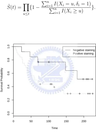
independent, the Kaplan-Meier estimator of S(t) can be written as ˆ S(t) =Y u≤t {1 − P_n i=1_PI(Xi = u, δi = 1) n i=1I(Xi ≥ u) }. 0 50 100 150 200 0.0 0.2 0.4 0.6 0.8 1.0 Time Survival Probability Negative staining Positive staining

Figure 1: K-M Survival Function

Figure 1.1 shows two Kaplan-Meier survival functions for two groups of patients. Notice that the two curves level off at the right tail and exhibit a stable plateau. Such a phenomenon is commonly seen in clinical trials and cancer studies. Whether there exists a group of subject who will never experience the event of interest despite long-term follow-up is an important scientific problem that requires subject-matter knowledge.

1.2

Mixture Model

Survival models in presence of immune or cured subjects have been extensively studied in statistical literature. The most popular approach is perhaps the mixture model formulation. Denote a binary variable ζ, where ζ = 1 indicates that the subject will experience the event of interest and ζ = 0 indicates that the subject will never experience the event no matter how large C is. For those susceptible ones with ζ = 1, T < ∞ with ˜S(t) = Pr(T > t|ζ = 1). For

those cured individuals with ζ = 0, T = ∞. The survival function of the whole population can be written as the following mixture form,

S(t) = P r(T > t|ζ = 1)P r(ζ = 1) + P r(∞ > t|ζ = 0)P r(ζ = 0)

= ˜S(t) · p + (1 − p),

where 1 − p = Pr(ζ = 0) is the cure rate. Under this model, the cumulative distribution of T becomes

F (t) = Pr(T ≤ t) = p(1 − ˜S(t)) = p ˜F (t),

and the hazard function can be written as

λ(t) = p ˜f (t)

1 − p + p ˜S(t),

where ˜f (t) is the density of T |ζ = 1. Usually ˜S(t) is called as the ”latency” survival function

for the susceptible group.

Cure models with the right censored observations suffer from an inherent identifiability prob-lem. Specifically the observation period should be long enough to make a judgment on the existence of cure. The book of Maller and Zhou (1996) contains detailed discussions on this issue under a non-parametric setting.

In most applications, covariate information is also available which would release the assump-tion on identifiability. Denote Z as a p × 1 vector of covariates. The data are of the form, (Xi, δi, Zi), i = 1, ..., n, where Zi is the covariate vector for the ith subject. Hence the mixture

model can be written as

S(t|Z) = P r(ζ = 1|Z)P r(T > t|ζ = 1, Z) + P r(ζ = 0|Z)P r(∞ > t|ζ = 0, Z)

= π(Z) ˜S(t|Z) + (1 − π(Z)).

The cure rate 1−π(Z) is often analyzed under a logistic regression assumption. In the landmark papers by Farewell (1982,1986), the Weibull distribution is imposed on the latency distribution. Other parametric models such generalized F distributions have also been proposed by Peng,

Dear and Denham (1998). Alternatively semi-paramertric regression models on the latency variable haven been studied. For example, the Cox proportional hazard (PH) model has been assumed by Kuk and Chen (1992), Peng and Dear (2000) and Sy and Taylor (2000), just to name a few. A more general class of semi-parametric transformation cure models has been considered by Lu and Ying (2004). It is suggested that, besides applying statistical methods to verify the identifiability condition, applications of cure models should be done with caution. One should check whether the result is consistent with medical or biological interpretation.

1.3

Outline of the Thesis

In the thesis, we will review some literature on survival models in presence of cure under the mixture formulation. We hope to provide a systematic way of studying different inference methods. Parametric analysis will be discussed in Chapter 2. Chapter 3 considers the likelihood approach for analyzing the Cox proportional hazard model and the linear transformation model. Methods developed based on some moment properties are discussed in Chapter 4. Concluding remarks are given in Chapter 5.

Chapter 2

Parametric Analysis

In this chapter, we examine the likelihood approach for estimating unknown parameters under a parametric setting.

2.1

Homogenous Data without Covariates

Suppose that observed data can be written as {(Xi, δi), i = 1, ..., n}, which are independently

and identically distributed replications of (X, δ), where X = T ∧ C and δ = I(T ∧ C). Assume that S(t) and f (t) can be indexed by Sθ(t) and fθ(t), where θ is the parameter of interest. In

absence of cure, the parametric likelihood of θ can be written as

n Y i=1 [fθ(xi)G(xi)]δi[Sθ(xi)g(xi)]1−δi ∝ n Y i=1 fθ(xi)δiSθ(xi)1−δi, (2.1)

where G(t) and g(t) is the survival and density functions of C respectively. The latter expression in (2.1) can also be represented by the hazard and survival functions as follows

L(θ) = n Y i=1 [λθ(xi)Sθ(xi)]δi[Sθ(xi)]1−δi = n Y i=1 λθ(xi)δiSθ(xi). (2.2)

In presence of cure, denote the latency density ˜f (t) as ˜fθ(t). The likelihood becomes a

function of θ and p which can be written as

L(θ, p) =

n

Y

i=1

[p ˜fθ(xi)]δi[p ˜Sθ(xi) + 1 − p]1−δi. (2.3)

The maximum likelihood estimator of (θ, p)T _{can be obtained by solving the two equations}

∂logL(θ, p) ∂θ = 0

and

∂logL(θ, p) ∂p = 0

given that the functions are differentiable with respect to (θ, p). It follows that

∂logL(θ, p) ∂p = n X i=1 δi p + n X i=1 (1 − δi) ˜ Sθ(xi) − 1 p ˜Sθ(xi) + 1 − p , ∂logL(θ, p) ∂θ = n X i=1 δi ˜ fθ(xi) ˜ f0 θ(xi) + n X i=1 p(1 − δi) p ˜Sθ(xi) + 1 − p ˜ S0 θ(xi), where ˜f0

θ(xi) and ˜Sθ0(xi) are partial derivatives of ˜fθ(xi) and ˜Sθ(xi) with respect to θ. Notice

that the score equations are complicated functions of p and θ since the two types of parameters need to be estimated jointly.

2.2

Parametric Analysis with Covariates

Suppose that observed data can be written as (Xi, δi, Zi), i = 1, ..., n. To model ζi = 1|Zi,

the following logistic regression model is often assumed:

pi(γ) = Pr(ζi = 1|Zi) = exp(Z0 iγ) 1 + exp(Z0 iγ) ,

where γ : q × 1 is the parameter vector. Suppose a parametric form is imposed on ˜f (t|Z) as

˜

fθ(t|Z). The likelihood function can be written as

L(θ, γ) =

n

Y

i=1

[pi(γ) ˜f |ziθ(xi)]δi[pi(γ) ˜S|ziθ(xi) + 1 − pi(γ)]1−δi. (2.4)

We will illustrate the likelihood analysis for two parametric models.Maximization of the likeli-hood function in (2.4) under the two models sometimes are quite complicated.

Farewell (1982, 1986) assumed that T |ζ = 1, Z follows a Weibull model such that its density function and survival function can be written as

˜

fθ(t|Z) = αλ(λt)α−1exp(−(λt)α),

where θ = (α, λ)T_{, λ = exp(−Z}0_{β) and}

˜

Sθ(t|Z) = Pr(T > t|ζ = 1, Z) = exp(−(λt)α).

Alternatively Peng, Dear and Denham (1998) applied the generalized F distribution to model the latency distribution. This parametric model is a flexible distribution which contains some useful distributions as special cases such as the Weibull and beta distributions. It is assumed that for those with ζ = 1, Y = log(T ) follows the generalized F distribution with the survival function

˜

Sθ(y|Z) = Pr(Y > y|ζ = 1, Z) =

Z _s2(s2+S1exp(yi−µ σ ))−1 0 xs2−1(1 − x)s1−1 B(s1, s2) dx, where ∞ < µ = Z0_{β < ∞, s}

1 > 0, s2 > 0, β is a vector of coefficients and B(s1, s2) is the beta

function with parameters s1 and s2. The resulting density function of Y is

˜

fθ(y|Z) =

(s1exp(yi−µ_σ )/s2)s1(1 + s1exp(yi−µ_σ )/s2)−(s1+s2)

B(s1, s2)

Farewell(1982) suggested to use Newton-Raphson method to maximize the log-likelihood. It requires computing inverse matrix of the second partial derivatives evaluated at the max-imum likelihood estimates. However for the generalized F distribution, it is impossible to derive the derivatives as closed-form expressions. This makes it difficult to apply the Newton-Raphson algorithm for solving the MLE. Peng, Dear and Denham (1998) suggested to combine a derivative-free maximization approach and the Newton-Raphson algorithm. Specifically they adopt the simulated annealing algorithm as the derivative-free maximization method to esti-mate the shape parameters. For fixed values of s1 and s2, the Newton-Raphson method is

Chapter 3

Semi-parametric Regression Analysis

- Likelihood Approach

In this chapter, we consider modeling T |ζ = 1, Z by semi-parametric regression models that contain un-specified functions as nuisance parameters.

3.1

Regression Models Without Cure

For illustration, we first introduce traditional regression models in absence of cure. The most well-known regression model in survival analysis is perhaps the proportional hazard model proposed by Cox (1972). Specifically given Z, the model be written as

λ(t|Z) = λ0(t) exp(Z0β), (3.1a)

where β : p × 1 is the unknown regression parameter of interest and λ0(t) is the baseline hazard

function. Another expression of the Cox model is given by

S(t|Z) = S0(t)exp(Z 0_β) = exp(− Z _t 0 λ(s|Z)ds) = exp(−Λ0(t) exp(Z0β)), (3.1b)

where Λ0(t) is the cumulative hazard function and S0(t) is the survival function for the baseline

group.

In recent years there is a trend to generalize different regression models under a unified framework. Notice that the Cox model can be written as

log(− log(S(t|Z))) = log(Λ0(t)) + Z0β. (3.1c)

We see that the right-hand side of (3.1c) shows a linear structure in the parameters log(Λ0(t))

and β. Similarly the proportional odds model can be written as

logit(S(t|Z)) = log S(t|Z) 1 − S(t|Z) = log[exp(Z 0_β) S0(t|Z) 1 − S0(t|Z) ]. It follows that logit(S(t|Z)) = logit(S0(t)) + Z0β. (3.2)

The two different models in equations (3.1c) and (3.2) are special cases of the following trans-formation models:

where h(·) is an unknown increasing function. Another expression of the model is given by

h(t) = −Z0_{β + ε, (3.3b)}

where ε is the error term with a known continuous distribution. The relationship between equations (3.3a) and (3.3b) is specified by

Fε(t) = Pr(ε ≤ t) = 1 − ϕ−1(t)

since

Fε(.) = Pr(ε ≤ t) = Pr(ϕ(S(T |Z)) ≤ t)

= Pr(S(T |Z) ≤ ϕ−1_{(t)) = Pr(1 − F (T |Z) ≤ ϕ}−1_(t))

= Pr[(1 − ϕ−1_{(t)) ≤ F (T |Z)] = 1 − ϕ}−1_(t).

Transformation models form a general class of regression models that have attracted substantial attention in recent years.

3.2

Regression Models In Presence of Cure

In presence of cure, recall that ζ|Z is modeled by

p(γ) = Pr(ζ = 1|Z) = exp(Z

0_γ)

1 + exp(Z0_γ).

Here we consider to model T |ζ = 1, Z by a transformation model such that

ϕ( ˜S(t|Z)) = h(t) + Z0β,

or equivalently

˜

S(t|Z) = ϕ−1_{(h(t) + Z}0_β).

Combining the two components, the survival function of T can be written as

S(t|Z) = p(γ) ˜S(t|Z) + (1 − p(γ))

= exp(Z0γ)

1 + exp(Z0_γ)S(t|Z) +˜

1

1 + exp(Z0_γ).

Notice that the cumulative hazard function of T |ζ = 1, Z can be written as ˜ Λ(t|Z) = − log[ ˜S(t|Z)] = −log[ϕ−1_{(h(t) + Z}0_{β)] = H(h(t) + Z}0_β). We can write S(t|Z) = exp(Z 0_{γ) exp[−H(h(t) + Z}0_{β)] + 1} 1 + exp(Z0_γ) = exp[Z0_{γ − H(h(t) + Z}0_{β)] + 1} 1 + exp(Z0_γ) .

Consider the example that T |ζ = 1, Z follows the Cox proportional hazard(ph) model with the hazard function and survival function

˜ λ(t|Z) = ˜λ0(t) exp(Z0β), ˜ S(t|Z) = Pr(T > t|ζ = 1, Z) = ˜S0(t)exp(Z 0_β) .

Accordingly the density function and survival function of T given Z can be written as

f (t|Z) = p(γ)˜λ(t|Z) × ˜S(t|Z), = p(γ)[˜λ0(t) exp(Z0β)] × ˜S0(t)exp(Z 0_β) , S(t|Z) = ˜S(t|Z)p(γ) + 1 − p(γ) = exp[−˜Λ0(t) exp(Z0β)]p(γ) + 1 − p(γ).

The major interest is to estimate β and γ while leaving ˜λ0(t) unspecified.

3.3

Likelihood Representations

The general form of likelihood function can be written as

n Y i=1 [pi(γ) ˜f (xi|zi)]δi[ ˜S(xi|zi)pi(γ) + 1 − pi(γ)]1−δi, (3.4a) or equivalently n Y i=1 [pi(γ)˜λ(xi|zi) ˜S(xi|zi)]δi[ ˜S(xi|zi)pi(γ) + 1 − pi(γ)]1−δi. (3.4b)

The second expression is useful when the model is expressed in terms of the hazard function such as the Cox model.

The likelihood approach has been applied to the Cox PH model in presence of cure by several authors. We have seen that the likelihood function is already quite complicated for analyzing parametric regression models. Now the challenge is to handle the infinite-dimensional nuisance function ˜λ0(t) in estimation. Specifically under the Cox model, we can write

L(γ, β, λ0(.)) = n Y i=1 [pi(γ)˜λ0(xi) exp(z0iβ) ˜S0(xi)exp(z 0 iβ)]δi [ ˜S0(xi)exp(z 0 iβ)p i(γ) + 1 − pi(γ)]1−δi.

3.4

Principle of the EM Algorithm

To apply the EM algorithm, we first need to construct the likelihood function based on ”complete data” {(xi, δi, zi, ζi), i = 1, . . . , n} assuming that ζi can be observed. Specifically the

likelihood function can be written as

LC = n Y i=1 [pi(γ) ˜f (xi|zi)]δiζi[ ˜S(xi|zi)pi(γ)](1−δi)ζi[1 − pi(γ)]1−ζi. It follows that LC = n Y i=1 (pi(γ)ζi(1 − pi(γ))1−ζi n Y i=1 ( ˜f (xi|zi)δiζiS(x˜ i|zi)(1−δi)ζi) = L1L2, (3.5)

where the likelihood function is divided into two parts. Notice that the first part L1 is a

function of γ which is the parameter for the cure rate model and the second part involves on the parameters for the latency distribution. This implies that the two types of parameters can be dealt with separately.

Since the value of ζi may be missing due to censoring, in the E-step, we calculate its expected

value given the observed data. It follows that

E[ζi|xi, δi, zi] = δi+ (1 − δi)Pr(ζi = 1|xi, δi = 0, zi). (3.6) Furthermore P r(ζi = 1|xi, δi = 0, zi) = P r(ζi = 1|Ti > xi, zi) = pi(γ) ˜S(xi|zi) pi(γ) ˜S(xi|zi) + 1 − pi(γ) . (3.7)

Detailed calculations of the above equation is given in Appendix 1. We see that equation (3.7) is a function of γ and ˜S(x|z) contains the nuisance function. In the M-step, we can maximize logL1 with respect to γ and logL2 with respect to the parameters in ˜S0(.) by replacing ζi by an

estimate of E(ζi|xi, δi = 1, zi) which is treated as a fixed constant by plugging in the parameter

estimates obtained previously. Numerical algorithms such as the Newton-Raphson method may be used in the maximization.

3.5

The EM Approach under the Cox Model

Now assume that T |ζ = 1, Z follows Cox PH model. The likelihood function is the product of the following two components:

L1(γ) =

n

Y

i=1

and L2(β, ˜λ0(.)) = n Y i=1 [˜λ0(xi) exp(zi0β)]δiζiexp[− Z _xi 0 ˜ λ0(t) exp(zi0β)dt]ζi. (3.9)

Recall that ζi will be replaced by the estimated value of its conditional expectation. The

maximization step of l1 is straightforward. To handle the nuisance function ˜λ0(.) in L2, we

introduce two approaches proposed by Sy and Taylor(2000) and Peng and Dear(2000). 3.5.1 Baseline estimation by Sy and Taylor

Actually two methods are proposed in the paper of Sy and Taylor (2000). The logarithm of equation (3.9) can be written as

l(β, ˜λ0(.)) = n X i=1 δiζi[log ˜λ0(xi) + zi0β] + n X i=1 ζi[−˜Λ0(xi) exp(zi0β)].

Assume that ˜Λ0(t) only jumps at observed failure points. Hence we can write

˜ Λ0(t) = n X i=1 I(tj ≤ t)˜Λ0(∆tj),

where tj is the jth observed failure point. Differentiating the log-likelihood with respect to

˜

Λ0(∆tj) for j = 1, . . . , k and setting the function as zero gives the following equation:

ˆ Λ0(∆tj) = dj P i∈R(tj)ζiexp(Z 0 iβ) ,

where dj is the number of failure at tj and R(t) is the risk set at time t. Accordingly

ˆ Λ0(t) = n X j=1 I(tj ≤ t)( dj P l∈R(tj)ζlexp(Z 0 lβ) ) (3.10)

which can be viewed as a modified version of the Breslow estimator if the value of β is known. Substituting ˆΛ0(∆tj) into L2(β, ˜Λ0(.)) leads to the following partial likelihood of β:

L3(β) = n Y i=1 (P exp(zi0β) l∈R(xi)ζlexp(z 0 lβ) )δi_{. (3.11)}

We can find the estimators of Λ0(t) and β are similar to the estimators obtained without cure

except that the weight ζl or its estimated conditional expectation is added to. The function

L3(β) does not contain any other nuisance function so that β can be estimated easily using the

traditional approach.

The above Breslow-type estimation separates the estimation of β and Λ0(∆tj). Sy and Taylor

An important technique is to express L2 based on ordered observed times t1 < . . . < tk.

Consider the interval [tj, tj+1). If xl ∈ [tj, tj+1) and δl = 1, the observation contributes the

probability ˜f (xl|zl) to the likelihood for the latency distribution. If xl ∈ [tj, tj+1) and δl = 0,

the observation contributes the probability ˜S(xl|zl) to the likelihood. Using the property that

˜ f (x) = ˜λ(x) ˜S(x), we have L2 = k Y j=1 {Y l∈Dj ( ˜f (xl|zl)ζl}{ Y l∈Cj ( ˜S(xl|zl)ζl} = k Y j=1 {Y l∈Dj (˜λ(xl|zl)ζl}{ Y l∈Ej ( ˜S(xl|zl)ζl},

where Dj is the set of subjects experiencing a failure event at time tj and Cj is the set of

subjects censored in [tj, tj+1) and Ej is the union of the two sets.

Define αi = Pr(T > ti|T ≥ ti, Z = 0, ζ = 1) which is the conditional survival probability at

time ti for the baseline susceptible subject. Then the baseline survival function ˜S0(t) can be

written as a product form of αi. Specifically

˜

S0(t) =

Y

j:tj≤t

αj.

Hence under the proportional hazard model ˜S(xl|zl) = ˜S0(xl)exp(z

0

lβ). Also

1 − ˜Λ(∆tj|z) = Pr(T > tj|T ≥ tj, z, ζ = 1) = (αj)exp(z

0 lβ).

The function L2(β, ˜Λ0(.)) can be written as

L3(β, α) = k Y j=1 [Y l∈Dj (1 − αexp(zl0β) j )ζl Y l∈Ej αζlexp(z0_lβ) j ]. (3.12)

Treating β as a constant and assuming that data have no ties, the MLE of αj can be written

as ˆ αj = (1 − exp(z0 jβ) P l∈R(tj)ζjexp(z 0 lβ) )exp(−z0 jβ). (3.13)

Substituting ˆαiinto the equation (3.12), a nonparametric profile likelihood of β can be obtained

and them maximized to get the MLE of β.

3.5.2 Baseline Estimation by Peng and Dear

Peng and Dear (2000) also suggested to use L3(β) for estimating β without dealing with the

the idea of Kalbfleisch and Prentice (1973) such that the survival function is expressed as the product of discrete hazard rates. The MLE of αj given β has the form,

ˆ αj ≈ 1 − dj P l∈R(tj)ζlexp(zlβ) .

3.6

Likelihood for Transformation Models

The likelihood function for linear transformation models with cure can be written as

L(γ, β, h(.)) = n Y i=1 [pi(γ) ∂ϕ−1_{[h(x) + z}0 iβ] ∂x |x=xi] δi ×[pi(γ)ϕ−1[h(xi) + zi0β] + (1 − pi(γ))]1−δi.

Note that for the Cox model, h(·) is related to the baseline hazard function which has clear properties that can be utilized to simplify the likelihood function. However for other trans-formation models, the role of h(·) is less clear. Therefore we will discuss methods constructed based on moment properties for transformation models.

Chapter 4

Semi-parametric Regression Analysis

- Moment-based Approach

As discussed in Chapter 3, a linear transformation regression model without cure has two equivalent expressions

h(T ) = −Z0_{β + ε}

ϕ(S(t|Z)) = h(t) + Z0_β,

where h(.) is an unknown increasing function and ϕ(.) is a known decreasing function related to the distribution of ε such that

Fε(t) = Pr(ε ≤ t) = 1 − ϕ−1(t).

When cure exists, we will assume that ζ = 1|Z follows a logistic regression model and

T |ζ = 1, Z follows a transformation model. We have S(t|Z) = exp(Z

0_γ)

1 + exp(Z0_γ)ϕ

−1_{(h(t) + Z}0_{β) +} 1

1 + exp(Z0_γ).

In this chapter, we discuss existing inference methods which utilize the moment principles.

4.1

Moment-based Inference: An Overview

The method of moment is attractive because it does not require strong distributional assump-tion and hence usually provides more robust results. Although the nonparametric likelihood approach is also robust, it is often very complicated for flexible models. Transformation models contain an un-specified function h(·) which complicates statistical inference.

Here we review some inference methods that are constructed using the idea of the method of moment. For example, denote Oi as a chosen response variable and Ei(θ) = E(Oi|Zi) as its

expected value, where θ is the parameter of interest. A moment-based estimating function has the form, U(θ) = n X i=1 Wi(Oi− Ei(θ)) = 0, (4.1)

where Wi is a weight function for ith subject. How to choose a suitable response Oi is the

key. If the response is well chosen, its expected value will be a nice function of the unknown parameters. For transformation models, we shall first pay attention to the form of Ei which

4.2

Response and its Expectation in Absence of Cure

For illustration, we first review exiting choices in absence of cure. There are three response variables. Specifically I(Ti ≥ Tj), i 6= j was proposed by Cheng et al.(1995), I(T ≥ t) by Cai et

al.(2000) and N(t) = I(T ≤ t) by Chen et al.(2002). We first examine their moment properties. 4.2.1 Pairwise Order Indicator

Temporarily assume there is no censoring and the data can be denoted as (Ti, Zi), i = 1...n.

Since h(.) is an unknown increasing function, it follows that

I(Ti ≥ Tj) = I[h(Ti) ≥ h(Tj)] = I(−Zi0β + εi ≥ −Zj0β + εj) = I(εi− εj ≥ Zi0β − Zj0β).

Then

E[I(Ti ≥ Tj)|Zi, Zj] = E[I(εi− εj ≥ Zi0β − Zj0β)] = Pr(εi− εj ≥ Zij0 β) = Φ(Zij0 β),

where Zij = Zi − Zj, Φ(s) =

R_∞

−∞[1 − Fε(t + s)]dFε(t) and Fε(.) is cumulative distribution

function for ε. More detailed derivations are given in Appendix 2. We have seen that h(·) disappear in the moment expression.

When censoring is present, observed data can be denoted as (Xi, δi, Zi), i = 1...n. Cheng et

al. (1995) suggested to use I(Xi ≥ Xj, δj = 1) as a proxy of I(Ti ≥ Tj). Note that as long

as the smaller observation corresponds to a failure point, the order relationship of the pair is known. However the proxy is biased since

E[I(Xi ≥ Xj, δj = 1)] = E[E[Ti ≥ Tj, Ci ≥ Tj, Cj ≥ Tj|Ti, Tj]] = E[I(Ti ≥ Tj)G2(Tj)],

where G(.) is the survival function of the censoring time. Weighting by the inverse-probability-of-censoring is often used to correct the bias and hence

E[δjI(Xi ≥ Xj) G2_(X j) |Zi, Zj] = E[I(Ti ≥ Tj)|Zi, Zj] = Φ(Zij0 β). In summary δjI(Xi ≥ Xj) G2_(X j)

is an unbiased proxy for I(Ti ≥ Tj).Detailed derivations are given

in Appendix 3.

4.2.2 The At-risk Indicator

Notice that h(·) still exists. When censoring is present, the corresponding response variable is

I(X ≥ t). It follows that

E(I(X ≥ t)|Z) = Pr(X ≥ t|Z) = ϕ−1_{[h(t) + Z}0_β]G(t).

To utilize this variable for further inference, how to construct high-dimensional estimating functions is crucial since the expected involves both β and h(·).

4.2.3 The Counting Process

Define the counting process N(t) = I(T ≤ t) and dN(t) = N(t) − N(t−) = I(T = t). The expected value of dN(t) conditional on the filtration Ft− is

E[dN(t)|Ft−]I(T ≥ t)λ(t)dt = Y (t)λ(t)dt = Y (t)dΛ(t).

Under the transformation model, we can write

Λ(t|Z) = − log S(t|Z) = − log{ϕ−1_{[h(t) + Z}0_β]},

E(N(t)|Ft−) =

Z _∞

0

Y (s)d[− log ϕ−1_{(h(s) + Z}0_β)].

In presence of censoring, the counting process is modified as N(t) = I(X ≤ t, δ = 1) and the at-risk process as Y (t) = I(X ≥ t). The conditional expectation of dN(t) given Ft− is similar

E(dN(t)|Ft−) = I(X ≥ t)λ(t)dt = Y (t)dΛ(t).

Under the transformation model, we have

E(N(t)|Ft−) =

Z _∞

0

Y (s)d[− log ϕ−1(h(s) + Z0β)].

which involves h(·) but does not contains G(·)

4.3

Estimating Functions in Absence of Cure

Now we illustrate how to construct estimating functions based on the moment properties. Recall that there are two types parameters, namely β and h(.). The former is of major interest. 4.3.1 Pairwise Order Indicator

Since the mean of I(Ti ≥ Tj) for i 6= j does not depend on the nuisance parameter, we have

the uncensored version

U(β) = n X i=1 n X j=1 W (Z0 ijβ)Zij × {I(Ti ≥ Tj) − Φ(Zij0 β)} = 0, (4.2)

and the censored version U(β) = n X i=1 n X j=1 W (Z0 ijβ)Zij × { δjI(Xi ≥ Xj) ˆ G2_(X j) − Φ(Z0 ijβ)} = 0, (4.3)

where ˆG(.) is the Kaplan-Meier estimator of G(.). The solution of U(β) = 0 yields an estimator

of β.

Although this approach is appealing since the nuisance parameter disappears, it has a crucial drawback when censoring is present. Notice that (4.3) has to be valid if P r(G(T ) = 0) = 0. This requirement however depends on the censoring mechanism. Define the following support points: τC = sup t t : G(t) = Pr(C > t) > 0, τT = sup t t : Pr(T > t) > 0, τX = sup t t : Pr(X > t) > 0.

It follows that τX = min(τT, τC). Problem occurs when τC < τT which implies the study period

is too short to observe large failure time. In this case the mean condition does not hold and hence the estimating functions is no longer unbiased.

4.3.2 The At-risk Event

Without censoring and from the previous moment derivation, a natural estimating equation is given by

n

X

i=1

(I(Ti ≥ t) − ϕ−1[h(t) + Zi0β]) = 0, (4.4)

for t ∈ [τa, τb], where τa, τb are pre-specified constants such that Pr(T < τa) > 0 and Pr(T <

τb) > 0. A set of equations for t being the observed values of Ti (i = 1, . . . , n) can be

con-structed which however are not enough since there are n + p unknown parameters since β is

p−dimensional. Cai et al.(2000) suggested the following additional estimating equations

n X i=1 {(I(Ti ≥ t) − E[I(Ti ≥ t|Zi)])} = 0, n X i=1 Z _τb τa Zi(I(Ti ≥ t) − ϕ−1[h(t) + Zi0β])dw(t) = 0, (4.5)

For right censoring data, we can construct two types of estimating equations: n X 1=1 (I(Xi ≥ t) − ϕ−1[h(t) + Zi0β] ˆG(t)) = 0, (4.6) and n X i=1 Z _τb τa Zi{I(Xi ≥ t) − ϕ−1[h(t) + Zi0β] ˆG(t)}dw(t) = 0. (4.7)

Numerical operation is same as mentioned above.

4.3.3 The Counting Process

Let (β0, h0(.)) be the true values of (β, h(.)). It is easy to see that

M(t) = N(t) −

Z _∞

0

Y (s)d[− log ϕ−1_(h

0(s) + Z0β0)

is a mean-zero martingale. This property can be used to construct estimating functions. The following is the proposal of Chen, Jin and Ying (2002):

n X i=1 dNi(t) − Yi(t)d[− log ϕ−1(h(t) + Zi0β)] = 0, (4.8) n X i=1 Z _∞ 0 Zi[dNi(t) − Yi(t)d[− log ϕ−1(h(t) + Zi0β)]] = 0. (4.9)

The first equation is for estimating h(.) at observed failure points and the second equation is for estimating β. The expressions of the estimating equations are similar when censoring is present.

4.4

Semi-parametric Transformation Cure Model

4.4.1 Estimating Functions

Semi-parametric inference for transformation models in presence of cure has been considered by Lu and Ying (2004) who constructed the estimating equations based on the counting process

N(t) mentioned above. In presence of cure, we have to modify

E(dN(t)|Ft−) = I(X ≥ t, δ = 1) Pr(T = t|T ≥ t) = I(X ≥ t, δ = 1)dΛ(t|Z)

, where Λ(t|Z) is the cumulative hazard function of T. Now we first derive the general form of Λ(t|Z) based on the model definitions and then discuss how to transform it into a more

tractable form. Recall that Λ(t|Z) = − log Pr(T > t|Z) and Pr(T > t) = Pr(ζ = 0|Z) + Pr(ζ = 1|Z) Pr(T ≥ t|ζ = 1, Z) = 1 1 + exp(Z0_γ)+ exp(Z0_γ) 1 + exp(Z0_γ)S(t|Z).˜

To create a linear pattern in unknown parameters, additional variable transformation is sug-gested. It follows that

˜

S(t|Z) = exp[−˜Λ(t|Z)] = ϕ−1_{(h(t) + Z}0_β),

where Fε(t) = Pr(ε ≤ t) = 1 − ϕ−1(t) and ˜Λ(t|Z) is the cumulative hazard function for

susceptible ones. Hence we let ˜

Λ(t|Z)] = − log{ϕ−1_{(h(t) + Z}0_{β)} = H(h(t) + Z}0_β).

Thus we can write

Pr(T > t) = 1 1 + exp(Z0_γ) + exp(Z0_γ) 1 + exp(Z0_γ)S(t|Z)˜ = 1 + exp(Z 0_{γ − H(h(t) + Z}0_β)) 1 + exp(Z0_γ) = 1 1 + exp(Z0_γ) 1 + exp(Z0_{γ − H(h(t) + Z}0_β)) 1 = ¯ψ(Z0_γ) 1 ¯ ψ{Z0_{γ − H[h(t) + Z}0_β]},

where ψ(x) = exp(x)/{1 + exp(x)} is the logistic function and ¯ψ = 1 − ψ. Using the fact that ψ(−x) = ¯ψ(x). We have

Λ(t|Z) = − log Pr(T > t|Z) = − log{ ¯ψ(Z0_{γ)} + log(ψ{−Z}0_{γ + H[h(t) + Z}0_{β]}). (4.10)}

It follows that M(t) = dN(t) − Y (t)d log ψ{−Z0_{γ + H[h(t) + Z}0_{β]} is a martingale when the}

parameters are evaluated at their true values. The suggested estimating functions have the forms

n

X

i=1

Note that equation (4.11) is used to estimate transformation function h(.) given β and γ eveluated at observed failure points of h(.) while equation (4.12) is for estimating β given h(.) and γ.

It should be noted that in presence of cure, we have additional unknown parameters γ but the above estimating functions are not sufficient to estimate the parameters in the logistic model. In Section 3.5, we have presented the log-likelihood function of γ given ζ is known.It follows that ∂l(γ) ∂γ = n X i=1 Zi[ζi − exp(Z0 iγ) 1 + exp(Z0 iγ) ] = 0. (4.13)

The imputation method is suggested to handle possible missingness of ζ. Specifically we impute

ζ by an estimator of E(ζ|X, δ, Z). The conditional probability that a subject belongs to the

susceptible group given that the subject with covariate Z is censored at X is ¯ψ{−Z0_{γ +H[h(t)+}

Z0_{β]}. So we get}

E(ζ|X, δ, Z) = δ + (1 − δ) ¯ψ{−Z0_{γ + H[h(t) + Z}0_{β]}. (4.14)}

The equation (4.13) can be modified as

n

X

i=1

Zi{δ + (1 − δ) ¯ψ{−Z0γ + H[h(t) + Z0β]}] − ψ(Zi0γ)} = 0. (4.15)

4.4.2 Estimation Algorithm

Solving (4.11), (4.12) and (4.15) jointly is not an easy task. Lu et al.(2004) proposed an iterative approach to obtain the solution. Recall that t1 < ... < tk be ordered failure points

and t0 = 0, tk+1 = ∞. Let di be the number of failure events at time ti. Denote the initial

value of β and γ as ˆβ(0) _{and ˆγ}(0) _{respectively which may be chosen as ˆγ}(0) _{= 0 and ˆβ}(0) _being

the maximum partial likelihood estimator under the ordinary Cox model as suggested by Lu et al.(2004). Denote ˆβ(m)_{, ˆγ}(m) _{and ˆh}(m)_{(t) are the mth estimated values. Let ˆh(·) be a step}

function taking jump at ti.

Step 1: This step involves solving of ˆh(tj) for j = 1, ..., k based on equation (4.11). With

ˆ β(m−1) _{and ˆγ}(m−1)_{, we obtain ˆh}(m)_(t k) by solving n X i=1 dNi(tk) − Yi(tk)dlog[ψ(H(ˆh(m)(tk) + Zi0βˆ(m−1)) − Zi0ˆγ(m−1)] = 0.

Step 2: Then based on equation (4.12), we update ˆβ(m) _{by plugging ˆh}(m)_{(t) and ˆγ}(m−1) _into the equation: n X i=1 Z _∞ 0 ZidNi(tk) − Yi(tk)dlog[ψ(H(ˆh(m)(tk) + Zi0β) − Zi0ˆγ(m−1))] = 0.

Step 3: Update ˆγ(m) _{based on the equation (4.15) such that}

n

X

i=1

Zi{δi+ (1 − δi) ¯ψ{−Zi0γˆ(m−1)+ H[ˆh(m)(tk) + Zi0βˆ(m)]} − ψ(Zi0γ)} = 0.

The procedure is implemented iteratively between the step 1 to step 3 until the convergence criteria is reached.

Chapter 5

Concluding Remarks

In this thesis, we review literature on cure mixture models. The likelihood can be simpli-fied by assuming complete data, which contains the indicator of susceptibility, are available. Then the EM algorithm can be applied. When the model assumption on the latency distribu-tion becomes more flexible, unknown parameters often involve infinite-dimensional funcdistribu-tions. Likelihood-based inference is usually constructed by expressing these functions as step-functions and hence the jump size at different points becomes the target in estimation. If the Cox model is assumed, existing partial likelihood method can be modified to account for the cure. How-ever for transformation models, the idea of method-of-moment is more attractive since the estimation procedure is more simple. Three forms of estimating functions are examined. The one based on the counting process has been extended to cure mixture models by Lu and Ying (2004). Despite its simplicity, efficiency of moment-type methods requires further investigation.

References

[1] Farewell, V. T. (1982),

The use of mixture models for the analysis of survival

data with long-term survivors. Biometrics 38, pp.1041-1046.

[2] Lawless, J. F. (1982), Statistical models and methods for lifetime data.

Wiley:New York.

[3] Farewell, V. T. (1986), Mixture models in survival analysis: are they worth

the risk? Can. J. Statist, 14, pp.257-262.

[4] Fleming, T. R. and Harrington, D. P. (1991), Counting processes and

sur-vival analysis. Wiley:New York.

[5] Kuk, A. Y. C. and Chen, C. H. (1992), A mixture model combining logistic

regression with proportional hazards regression. Biometrika, 79, pp.

531-541.

[6] Maller, R.A. and Zhou, S. (1992), Estimating the proportion of immunes

in a censored sample. Biometrika, 79, pp. 731-739.

[7] Chen, S. C., Wei, L. J. and Ying, Z. (1995), Analysis of transformation

models with censored data. Biometrika,82, 4, pp. 835-845.

[8] Maller, R.A. and Zhou, S. (1996), Survival analysis with long-term

sur-vivors. Wiley:New York.

[9] Peng, Y. W., Keith B. G. Dear and Denham, J.W. (1998), A generalized

F mixture model for cure rate estimation. Statistics in Medicine,17, pp.

813-830.

[11] Cai, T., Wei, L. J. and Wilcox, M. (2000), Semiparametric regression

anal-ysis for clustered failure time data. Biometrika,87, 4, pp. 867-878.

[12] Chen, K., Jin, Z. and Ying, Z. (2002), Semiparametric analysis of

trans-formation models with censored data. Biometrika,89, 3, pp. 659-668.

[13] Lu, W. and Ying, Z. (2004), On semiparametric transformation cure

Appendix

A1. Derivation of E(ζi|(xi, δi = 0, zi))

E(ζi|(xi, δi = 0, zi)) = P r(ζi = 1|Ti > xi, zi) = P r(ζi = 1, Ti > xi|zi) P r(Ti > xi|zi) = P r(ζi = 1|zi)P r(Ti > xi|ζi = 1, zi) P r(ζi = 1|zi)P r(Ti > xi|ζi = 1, zi) + P r(ζi = 0|zi)P r(∞ = Ti > xi|ζi = 1, zi) = P r(ζi = 1|zi)P r(Ti > xi|ζi = 1, zi) P r(ζi = 1|zi)P r(Ti > xi|ζi = 1, zi) + P r(ζi = 0|zi) = π(zi) ˜S(xi|zi) π(zi) ˜S(xi|zi) + 1 − π(zi) . A2. Derivation of Φ(s) = P r(εi− εj ≥ s) Let V = εi− εj, εi.i.d∼ fε, Φ(s) = P r(εi− εj ≥ s) = Z _∞ s Z _∞ −∞ fεi,εj(v + εj, εj)dεjdv = Z _∞ s Z _∞ −∞ fε(v + εj)fε(εj)dεjdv = Z _∞ s Z _∞ −∞ fε(v + εj)dFε(εj)dv = Z _∞ −∞ Z _∞ s fε(v + εj)dvdFε(εj) = Z _∞ −∞ (1 − Z _s −∞ fε(v + εj)dv)dFε(εj) = Z _∞ −∞ (1 − Fε(s + εj))dFε(εj) = Z _∞ −∞ (1 − Fε(s + t))dFε(t).

A3. Derivation of E[δiI(Xi≥Xj) G2_(Xj) |Zi, Zj] E[δiI(Xi ≥ Xj) G2_(X j) |Zi, Zj] = E[ I(Cj ≥ Tj)I(Xi ≥ Xj) G2_(X j) |Zi, Zj] = EE[I(min(Cj, Xi) ≥ Tj) G2_(T j) |Zi, Zj, Tj]

= EE[I(min(Cj, Ci) ≥ Tj)I(Ti ≥ Tj)

G2_(T j) |Zi, Zj, Tj] = EE[I(min(Cj, Ci) ≥ Tj) G2_(T j) E[I(Ti ≥ Tj)]|Zi, Zj, Tj] = E[E[I(Ti ≥ Tj)]|Zi, Zj, Tj] = E[I(Ti ≥ Tj)|Zi, Zj] = Φ(Zij0 β).