結合次頻帶適應性濾波與變步長正規最小均方演算法的迴音消除技巧

!

!

#

$

%

&

'

"

()*+,-.'/"

0

"

1

"

2

"

3

"

456789:;<=*>?@ABCDEFGHIJKL

MNOP"

"

QRSSTUV"WVTXYZ[\"]Z^Y\_ZU`"aZYb"cT_ZTS^\"QY\XdQZe\"fghQ"ij_"klbj"mTUl\^^TYZjU"

"

n"o"pqrst"

uvwxqyz{""|1"

"

"

}"~"•"! "€"•"‚ "ƒ"„"…"

!

"#$%&'()*+,-./0123456789:;<=>?!

@ABCDE

FGHIBJKL!

MNOPQ@RS,TUVW@XYZ[\]^_`!

a

! ! ! ! ! !

b

!

cdefghijklmcn-ophq@:;<=9rstcuvwx'

()*+>y9Z[iz{|}~$%&'()*+>y•€•‚ƒ„9…†

„‡tˆ‰Š'()*+>y(‹Œ$%&i•Ž•€•‚•‘9’7“t”

•5–i012345678"#-./Ž—}~{cn-oph•‚˜™9

š›{œt•ži-./012345678(‹cŸ%'()*+ ¡i•

9¢‹P£¤¥¦’7“9tcdefgijkŠ-./012345678

(‹§¢‹¨©ª%«¬-®¯°-*+ ±²$%&'()*+tjkŽ³

´µjk\¶·9589¸¹º~t»¼Š³½~jk\¶·958¾¿š›

{œÀ…†„‡ÁnŽ•‚‘“9’7ÂÇt!!

!

Ä

! ! ! ! ! !

Å

ÆÅFGHI!JKLÇÈÉcÊË9Z[\Ì@uWÍiÎÏjÐÑ9F

GiÒÓjÔÕÖ×ØÙ9Z[¹‡tÆÅÚÛÜ@/ÝÞ²ÍßàÎÏjf

g¡9FGiÓj{áâãäfgtåæÆÅçèéêJëìHIcçèÍí

îefg\¶·9ïðiÓdefgñòãót!

ÆÅôõö÷ø€ùúûicjüýþÿ!"n˜#$%&FGjc'(¡

9rsiÓjLÆ)*tÆÅï+c,ÊË-•.¶/j0§1(i{2§3

45967-¤8’tÆÅ9:cZ[\A;Àj<Áä/i=>jª8?3

•@ABCDE_@7iF{G3áâH§@7tÆÅIJ9KLùMÕiÓ

j{cNOPÑ&ýQj9Z[VRtÆÅS!cjTRfgUV•0WXY

4iÒZcj[\nÎÏì]i‘^nÎÏ_`iWjau,•wt!

Subband Adaptive Filtering with Variable

Step-Size NLMS for Echo Cancelation

Tsung-Yao Chiang

Advisor: Dr. Yuan-Pei Lin

Department of Electrical and Control Engineering

National Chiao Tung University

September 3, 2007

Abstract

In this thesis, we consider the problem of acoustic echo cancelation for a time varying environment. In the context of adaptive filtering, the subband adaptive filtering (SAF) is known to enjoy a fast convergence rate. By applying adaptive filtering in the subbands, it also has the advantage of a lower complexity. On the other hand, the normalized least mean squares (NLMS) algorithm with a variable step size (VSS) is known to have a good tracking ability in a time varying environment. However the implementation of VSS-NLMS is usually computationally expensive as it is applied to fullband adaptive filter. In this thesis, we apply VSS-NLMS to the subband filters using a approximately alias-free cosine modulated filter bank. We also analyze the steady state behavior of the proposed algorithm. Simulations show that the proposed method achieves a good trade-off between tracking performance and convergence rate while having a low computational complexity.

Contents

1 Introduction 1

1.1 Outline . . . 3

1.2 Notations . . . 3

2 System Model 5 3 Subband Adaptive Filters 8 3.1 Input and Output Relationship of SAF . . . 8

3.2 Subband Adaptive CMFB . . . 10

3.3 Computational Complexity of SAF with AAFCMFB . . . 13

4 Variable Step-Size NLMS [9] 17 4.1 VSS-NLMS algorithm . . . 17

4.2 Performance Analysis . . . 19

5 SAF using AAFCMFB with VSS-NLMS 22 5.1 SAF with VSS-NLMS Algorithm . . . 22

5.2 Performance Analysis . . . 25

5.2.1 Mean-Squared Value of Weight error Vector . . . 26

5.2.2 Steady-State Behavior . . . 31

6 Simulation 33

7 Conclusion and Future work 49

List of Figures

2.1 Teleconference system. . . 6

2.2 Teleconference system with mobile phone. . . 6

2.3 Adaptive filter . . . 7

2.4 Subband adaptive filters . . . 7

3.1 Structure of subband adaptive filtering. . . 9

3.2 Frequency response of first M analysis(synthesis) filters. . . 11

3.3 Frequency response of last M analysis(synthesis) filters. . . 12

3.4 Implementation of analysis bank of 2M-band AAFCMFB with DCT matrix. . . 14

6.1 Fullband NLMS with color input sequence in a nonstationary en-vironment. . . 35

6.2 Fullband NLMS with white input sequence in a nonstationary en-vironment. . . 35

6.3 Impulse responses of echo paths with different position of room, where the microphone leaves 6 centimeters of loudspeakers in (a) and the microphone leaves 30 centimeters of loudspeakers in (b) . 37 6.4 one person stand near the speaker initially, and walks straight with velocity 0.707m/s at first 4 seconds, then stay here for 4 seconds 38 6.5 the person stay near the speaker at first 4 seconds, and walks straight with velocity 0.707m/s for 4 seconds. . . 38

6.6 one person stand near the speaker initially, and walks along the wall with velocity 0.5m/s at first 2 seconds, and then turns right for 2 seconds. Finally, stay here for 4 seconds . . . 39

6.7 Learning curves under SNR 20dB when the echo path is according to Fig. 6.4 . . . 40 6.8 Learning curves under noise absent when the echo path is according

to Fig. 6.4 . . . 40 6.9 Learning curves under SNR 20dB when the echo path is according

to Fig. 6.5 . . . 41 6.10 Learning curves under noise absent when the echo path is according

to Fig. 6.5 . . . 41 6.11 Learning curves under SNR 20dB when the echo path is according

to Fig. 6.6 . . . 42 6.12 Learning curves under noise absent when the echo path is according

to Fig. 6.6 . . . 42 6.13 Learning curves of proposed method with different initial step size

under SNR 20dB when the echo path is according Fig. 6.4 . . . . 44 6.14 Learning curves of proposed method with different initial step size

under noise absent when the echo path is according Fig. 6.4 . . . 44 6.15 Learning curves of proposed method with different initial step size

under SNR 20dB when the echo path is according Fig. 6.5 . . . . 45 6.16 Learning curves of proposed method with different initial step size

under noise absent when the echo path is according Fig. 6.5 . . . 45 6.17 Evolutions of the step size of Fig. 6.14 with different initial value. 46 6.18 Evolutions of the step size of Fig. 6.16 with different initial value. 46 6.19 Evolutions of the step size with white input in different α =

−0.76, −0.3, 0, 0.3, 0.76, and the initial value of step size is 0.4. . . 47 6.20 Evolutions of the step size with white input in different α =

−0.76, −0.3, 0, 0.3, 0.76, and the initial value of step size is 1.4. . . 47

6.21 Evolutions of the step size with color input in different α = −0.76, −0.3, 0, 0.3, 0.76, and the initial value of step size is 0.4. . . 48

6.22 Evolutions of the step size with color input in different α = −0.76, −0.3, 0, 0.3, 0.76, and the initial value of step size is 1.4. . . 48

A.1 The graph of f (α) vs. α. The 5 circles denote 5 zeros of f (α) and the dash lines are asymptotes. x is α, y is f (α) . . . 54

List of Tables

3.1 Computational complexity per input signal, where M is the num-ber of decimation and L is the length of fullband adaptive filter . 16 5.1 Computational complexity of VSS per input signal, where M is

the number of decimation and L is the length of fullband adaptive filter . . . 25

Chapter 1

Introduction

In acoustic echo cancelation (AEC), the echo path usually has thousands of taps [1]. Hence it is necessary to model the echo path by using a filter with thousand of taps. In this case the computational complexity is large and the convergence rate is slow [2]. This motivates the use of subband adaptive filtering (SAF) techniques, which can achieve computational efficiency by decimating the signals before performing the adaptive filtering. Many research has been done as follows. In [3], an analysis of multirate concept for AEC is presented. An optimum filter banks which minimize the aliasing distortion was introduced in [4]. In [5], a new type of subband adaptive filters (SAFs) architecture that avoids signal path delay while retaining the computational and convergence speed advantages of subband processing was proposed. A computationally efficient way for approximating the filter banks was introduced in [6] for subband identification. In [7], approximately alias-free cosine modulated filter banks (AAFCMFB) was presented, which has real coefficients and is almost aliasing-free. Thanks to its lower computational complexity and approximately free aliasing property in this thesis, we will use SAFs with approximately alias-free cosine modulated filter bank [7].

In addition to the long echo length issue, the echo environment is usually time varying, and hence the echo path is time varying. In this case, the tracking abil-ity becomes more important. Although the SAFs have faster convergence rate, the tracking performance is usually unsatisfactory. To improve the tracking per-formance while keeping the fast convergence rate, a number of variable step-size

algorithm have been developed, e.g., [8]-[10]. The main idea of variable step size is to reduce the conflict between the convergency rate and tracking performance. Mathews [8] proposed to adaptively change the step-size of the LMS algorithm. The variable step size is proportional to the negative gradient of the instant squared error. Base on [8], Sulyman [9] used Mathews’s idea to the NLMS algo-rithm. The above papers assume the input signal is white. However, in practice, input signal is in general colored and these methods do not work well in this case. To overcome this, Liu [10], Diniz [11] and Sristi [12] proposed to use SAFs with variable step-size, because SAFs can divide the input sequence to several bands and the signal is in each band is relatively white. When the number of bands is sufficiently large, it becomes approximately white. However, Liu’s algorithm requires higher computational complexity to adapt the variable step-size than Mathews’s algorithm. Moreover, the coefficients of the filter banks are complex-value, which leads to large computational complexity. Diniz’s method needs to estimate correlation matrix and his filterbanks contains cross filter, which in-crease complexity. Sristi’s method requires three extra parameters, and the value of parameters need to be choose carefully or the performance will be destroyed.

To reduce the complexity of variable step-size SAF, in this thesis, we propose to use AAFCMFB in the SAF [7] and use Sulyman’s method [9] for variable step size adaptation, because Sulyman’s method requires less computation complexity as we will analyze in Chapter 4 and AAFCMFB can be implemented with real co-efficients and the efficient discrete cosine transform (DCT) structure. Moreover, we analyze the performance of the proposed method and derived the steady-state MSE. Furthermore the comparison of computational complexity for the proposed method and the conventional schemes is also presented. Finally, simulation re-sults show that the speech correlation does not affect tracking performance and the proposed method not only achieves good tracking performance but also do not destroy the property of fast convergence rate. The thesis is organized as follow.

1.1

Outline

• Chapter 2: System model is presented.

• Chapter 3: We review SAFs , such as filterbank structure, aliasing function and subband adaptive algorithm. Then, the AAFCMFB is introduced. We will present the structure of AAFCMFB first. Then we derive that the aliasing can be eliminates by proper choosing subband adaptive filters. • Chapter 4: The introduction of variable step-size NLMS is present. In sec.

4.1, we describe the VSS-NLMS algorithm. In sec. 4.2, derivation of MSE will show here.

• Chapter 5: The combination of VSS-NLMS and AAFCMFB is presented. In sec. 5.1, the method to adapt the step size is described. In sec. 5.2, we will analyze the performance of VSS-SAF, such as convergence rate and steady state mean square error (MSE).

• Chapter 6: We will compare the experimental results of AF and SAF using AAFCMFB with fixed step-size and variable step-size for the environments under different walkpaths and SNR Levels.

• Chapter 7: Conclusion.

• Appendix A The range of step-size for stability • Appendix B Behavior of weight-error vector

1.2

Notations

1. The lower-case letters represent scalar values.

2. The lower-case and upper-case letters whit hold face represent vector and matrix quantities.

4. WM is defined as e−j

2π M.

5. The notation IM is used to represent the M × M identity matrix.

6. The notation CM is used to represent the M × M DCT matrix given by [CM]_ij = cos

! π

M(i + 0.5)j "

, 0 ≤ i, j < M. 7. The notation ΓM is defined as

[ΓM]_ij = #

−1i _{while i = j,}

0 otherwise.

where, 0 ≤ i, j < M.

8. The notation JM is defined as [JM]_ij =

#

1 while i = M − j, 0 otherwise.

Chapter 2

System Model

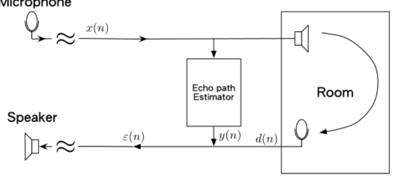
We first describe acoustic echo cancelation by the teleconference system as shown in Fig. 2.1. The speech of the far end user is transmitted to the near end user, and vice versa. At the near end, the microphone and the speaker are set in the same room, so the far end user will receive not only the speech from the near end user but also the signal caused by the speech from the far end user. Here we define the acoustic echo as the speech of the far end user transmitted back to the far end terminal. The echo can be generated by passing the speech of the remote user through the echo path. The echo path can be estimated by echo path estimator as shown in Fig. 2.1. After each path estimation, we can generate the echo signal y(n) by passing the speech of the remote user through the echo path. If we subtract the echo from the signal which is transmitted back to remote terminal, the acoustic echo can be canceled. Let us consider the time-variant teleconference system as shown in Fig. 2.2. It is almost the same as the system in Fig. 2.1 except that the microphone of the near end user is mobile. As a result, the echo path is time-variant.

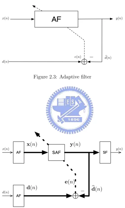
Because the echo path is time-variant now, we should consider the convergency rate and the steady state error as well as the tracking performance. Fig. 2.3 shows an echo path estimator. For convenience, we call it adaptive filter or fullband adaptive filter. The block with abbreviation ”AF” denotes adaptive filter which adapts according to given adaptive algorithm, such as LMS, NLMS and RLS [2]. Fig. 2.4 shown the structure of a SAF, where x(n), d(n) and y(n) represent

!""# $%&"'()*&'

$+*,#)*"-≈

≈

Figure 2.1: Teleconference system.

!""# $%&"'()*&'

$+*,#)*"-≈

≈

Figure 2.2: Teleconference system with mobile phone.

the same signal as that in Fig. 2.3. This structure not only can reduce the computational complexity but also accelerate the convergence rate as we will have more detailed explanation later.

x(n) y(n)

d_(n)

!"

+

e(n) _d!_(n)

Figure 2.3: Adaptive filter

x(n) y(n) d_(n) !" !" #" #!"

+

Chapter 3

Subband Adaptive Filters

Many different SAFs have been proposed to countervail echo noise.There are two reasons to use SAF: First, the echo path of a room has long impulse response. If conventional AF is used to overcome this issue, it demands high computational complexity due to large taps of adaptive filter. By using SAF with decimation, the computational complexity can be reduced. Hence, real-time AF can be realized. Second, the frequency response of a echo path is usually frequency selective and the energy of echo concentrates in low frequency band. If we use SAF and adapt only the bands which contain higher energy, the computation complexity can again be reduced. Moreover it will not cause significant error.

3.1

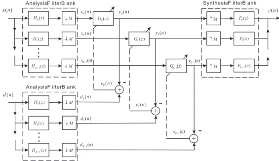
Input and Output Relationship of SAF

Fig. 3.1 is a detailed structure of SAFs . The input signal x(n) is filtered by the analysis filters Hk(z) in the kth subband, decimated by a factor M, and resulting in the subband signals xk(n), which is the input signals of the subband filters Gk(z). Subband filter Gk(z) is the adaptive filter of kth subband. Subband signal dk(n) is the desired signal of the kth subband filter and resulted by desired signal d(n) in the same way. Subband signals yk(n),which is the output signals of the subband filters, are interpolated by the factor M, filter by the synthesis filters Fk(z), and add together to form the output signal y(n). ek(n) is the error signal of kth subband.

) ( 0z H ) ( 1z H ) ( 1z HK !

!

!

AnalysisF ilterB ank

AnalysisF ilterB ank

SynthesisF ilterB ank

-Figure 3.1: Structure of subband adaptive filtering.

can be expressed respectively as xk(n) = x(t) ∗ hk(t)   t=M n, 0 ≤ k ≤ K − 1, (3.1) and Xk(z) = 1 M M−1_% !=0 Hk(z 1 MW! M)X(z 1 MW! M), 0 ≤ k ≤ K − 1. (3.2) The subband signals is passed through the subband filters, upsampled by M and composed by synthesis filter banks. Then Y (z) can be expressed as

Y (z) = 1 M K−1_& k=0 M−1_& m=0 Hk(zWMm)X(zWMm)Gk(zM)Fk(z) = 1 M M−1_& m=0 K−1_& k=0 Hk(zWMm)Gk(zM)Fk(z)X(zWMm) = M−1_& m=0 Tm(z)X(zWMm), (3.3) where Tm(z) = 1 M K−1_% k=0 Hk(zWMm)Gk(zM)Fk(z). (3.4) Tm(z) is defined as the transfer function. More specifically, T0(z) is the distortion function and Tm(z), m %= 0, is the aliasing function. If the aliasing function is

approximately zero, i.e.,

Tm(z) ≈ 0, ∀ 1 ≤ m ≤ M − 1, (3.5)

we can simplify (3.3) to

Y (z) = T0(z)X(z). (3.6)

If the output signal is the delayed version of the input signal with delay τ , i.e., y(n) = cx(n − τ), where c is a constant, we say that such a filterbank is perfect reconstruction (PR).

3.2

Subband Adaptive CMFB

CMFB has lower complexity than the filter banks with complexity coefficients because all the signal processing of CMFB is realized by real-valued computation. The CMFB has the alias-free property. However, when CMFB is used as the analysis and synthesis filter bank in Fig. 3.1 due to the insertion subband filters, the aliasing-free property will be destroyed. In [7], SAFs with AAFCMFB has been presented. The decimation factor of AAFCMFB is half of the number of subchannels. The AAFCMFB contains not only cosine modulation (first half of subbands) but also sine modulation (last half of subbands). By properly choosing subband filter, alias-free property for AAFCMFB can be achieved.

In both CMFB and AAFCMFB, all the filter of AF and SF are constructed by a prototype filter. The procedure of filter construction is described below. First , we design a prototype filter P (ejω_{). Such filter is a lowpass filter with} bandwidth _Mπ + $. Second, we define a piece wise band filter

Pk(z) = P (zW2Mk+0.5) , where W2Mm = ej

2πm

2M . (3.7)

Third, define the analysis filters as: Hk(z) =

#

Pk(z) + P2M −1−k(z) , 0 ≤ k ≤ M − 1 −jPk(z) + jP2M −1−k(z) , M ≤ k ≤ 2M − 1.

(3.8) Finally, the synthesis filters are obtained by time reversing the analysis filters, i.e.

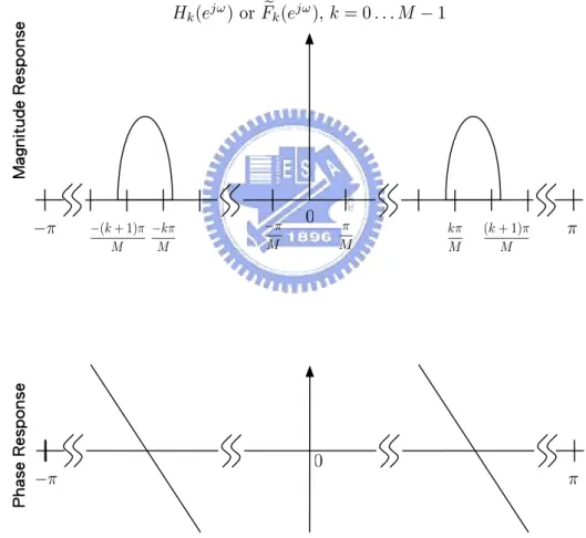
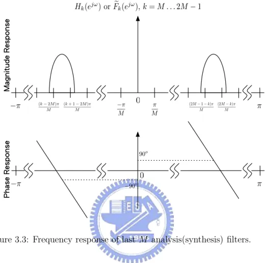
If the prototype filter has real coefficients, the frequency response of the first M analysis/synthesis filters are even functions of ω (cosine modulation), and the last M ones are odd functions of ω (sine modulation), so that all analysis/synthesis filters have real coefficient. With real coefficients, we can process the signal by real-value addition and multiplication, which can reduced the complexity by half when compared with complex computations. Fig. 3.2 and Fig. 3.3 show two frequency response of analysis/synthesis filter, whose prototype filter has linear phase. H_k(ejω_{) or !F} k(ejω), k = 0 . . . M − 1 −(k+ 1)π M (k + 1)π M −kπ M kπ M −π M π M π −π 0 0 π −π !" #$% &'( )*+ ), -.$, ) /0" , )*+ ), -.$, )

0 π −π 90o −90 o H_k(ejω_{) or !}F_k(ejω_{), k = M . . . 2M − 1} 0 −π M π M π −π (k + 1 − 2M )π M (k − 2M )π M (2M − k)π M (2M − 1 − k)π M !" #$% &'( )*+ ), -.$, ) /0" , )*+ ), -.$, )

Figure 3.3: Frequency response of last M analysis(synthesis) filters.

Substituting (3.8) and (3.9) into (3.4), the transfer function becomes Tm(z) = _M1 2M −1_& k=0 Hk(zWMm)Gk(zM)Fk(z) = _M1 _{ M_&−1 k=0 [Pk(zWMm) + P2M −1−k(zWMm)]Gk(zM)[ 'Pk(z) + 'P2M −1−k(z)] +2M −1& k=M [Pk(zWMm) − P2M −1−k(zWMm)]Gk(zM)[ 'Pk(z) − 'P2M −1−k(z)]}. (3.10) If we choose Gk(z) = G2M −1−k(z), the transfer function becomes [7]

Tm(z) = 2 M M−1_% k=0 [Pk+2m(z) 'Pk(z) + P2M −1−k+2m(z) 'P2M −1−k(z)]Gk(zM). (3.11) Using the fact that prototype filter satisfies

and substituting z = z"_Wl

2M, l is a integer, into (3.12), we have

P (z"_W2m+l 2M ) 'P (z"W l 2M) ≈ 0, for 1 ≤ m ≤ M − 1, (3.13) i.e. Pl+2m(z) 'Pl(z) ≈ 0, for 1 ≤ m ≤ M − 1. (3.14) Substituting (3.14) into (3.12), We will see all the aliasing function is approxi-mately zero, and the distortion function is given by

T0(ejω) = 2 M M_%−1 k=0 () )Pk(ejω) ) )2 +))P2M −1−k(ejω) ) )2* Gk(ejM ω). (3.15)

3.3

Computational Complexity of SAF with AAFCMFB

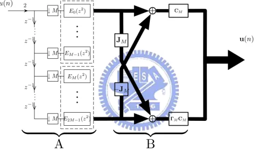
Referring to Fig. 3.1, when the AAFCMFB is used as the analysis and synthesis filter banks, the analysis filterbank can be expressed by the polyphase components of prototype filter[13], i.e.

Hk(z) = # P (zW_2Mk+0.5) + P (zW_2M−(k+0.5)) _{, 0 ≤ k ≤ M − 1} −jP (zW2Mk+0.5) + jP (zW −(k+0.5) 2M ) , M ≤ k ≤ 2M − 1 =                        2M −1_& l=0 El / (zW_2Mk+0.5)2M0_(zWk+0.5 2M )−l +2M −1& l=0 El ! (zW_2M−(k+0.5))2M"_(zW−(k+0.5) 2M )−l , 0 ≤ k ≤ M − 1 −j 2M −1_& l=0 El / (zW_2Mk+0.5)2M0_(zWk+0.5 2M )−l +j 2M −1_& l=0 El ! (zW_2M−(k+0.5))2M"_(zW−(k+0.5) 2M )−l , M ≤ k ≤ 2M − 1 =        2M −1_& l=0 El(z2M)z−l ! 2 cosπ(k+0.5)l_M " _{, 0 ≤ k ≤ M − 1} 2M −1_& l=0 El(z2M)z−l ! 2 sinπ(k+0.5)l_M " _{, M ≤ k ≤ 2M − 1,} (3.16) where El(z) represents the Type 1 polyphase components of the prototype filter P (z)

P (z) =

2M −1_%

l=0

Referring to Fig. 3.4, we can construct the analysis filter banks of AAFCMFB by DCT matrix and the polyphase components of prototype filter [13]. The signal pair {u(n), u(n)} can be {x(n), x(n)} or {d(n), d(n)}, where the elements of x(n) is subband signals xk(n) and the elements of d(n) is subband signals dk(n). When we reverse the direction of signals in 3.4, it becomes a synthesis filter banks and the signal pair {u(n), u(n)} is {y(n), y(n)}, where the elements of y(n) is subband signals yk(n). The computational complexity can be greatly reduced due to this efficient implementation. Using the efficient implementation of AAFCMFB as in

+ + 2 z−1 z−1 z−1 z−1 z−1 . . . . . .

.

.

.

.

.

.

A

B

!

"#

$

!

"#

$

Figure 3.4: Implementation of analysis bank of 2M-band AAFCMFB with DCT matrix.

Fig. 3.4, it requires much fewer multiplications. The complexity of SAF using AAFCMFB without considering adaptation is calculated as follow:

Without Adaptation

• Let us discuss the complexity in part A.The complexity of a polyphase component is Lproto

M , where Lproto is the length of prototype filter. Assume that there are N input signals, the symbol passing to each polyphase com-ponents is N

M. Thus the complexity for 2M polyphase components are N M × Lproto M × 2M = 2N Lproto M

• The complexity of a DCT matrix is M log2M [14], and that of diagonal matrix ΓM is M. Assume that there are N input signals, the number of symbols passing to DCT matrix is N

M. The complexity of DCT matrix is M log2M and the complexity of DST matrix is M log2M + M, the extra complexity M is caused by ΓM. Then the complexity of part B is _MN × (2M log₂M + M) = N(2 log₂M + 1).

• Referring to Fig. 3.1, the complexity of subband filters for N input signals are N

M ×

L

M × 2M =

2N L

M , where L/M is the length of subband filter. • Referring to Fig. 3.1, the complexity of the synthesis filter bank is the same

as that of the analysis filter bank.

According to [7], the update equation of the coefficient of the first k subband filters based on the NLMS algorithm are

gk(n) = gk(n − 1) + µ

xk(n − 1) (xk(n − 1)(2

ek(n − 1), k = 0 . . . M − 1, (3.18) and the other subband filters does not adapt and are obtained by

gk(n) = g2M −1−k(n), k = M . . . 2M − 1. (3.19) Let the length of subband filter be L

M. The complexity of adaption for SAF using AAFCMFB is calculated as:

Adaptation Only

• To calculate (xk(n)(2 of the kth subband filter, we need _ML multiplications. Then M subband filters need L multiplications.

• To calculate µek(n)

#xk(n)#2, we need 2 multiplications. Then M subband filters

needs 2M multiplications. • The production of µek(n)

#xk(n)#2 and xk(n) needs

L

M multiplications. Then M subband filters need L multiplications.

Filtering Adaption SAF using AAFCMFB 6Lproto

M + 6 log2M + 3 +2LM 2( L

M + 1)

Fullband AF L 2(L + 1)

Table 3.1: Computational complexity per input signal, where M is the number of decimation and L is the length of fullband adaptive filter

• From above, one adaption needs 2L + 2M multiplications. However, the number of adaption for SAF is only 1

M of the case for Fullband AF. That is, we have one adaptation for M input signals. Hence, for one input signal, we only need 2L+2M

M multiplications.

The comparison of computation complexity for SAF using AAFCMFB with DCT and fullband AF is given in Table 3.1. Later, we will give an example in Chapter 6 to illustrate the complexity reduction using AAFCMFB with DCT matrix.

Chapter 4

Variable Step-Size NLMS [9]

In this chapter, we review VSS-NLMS algorithm. The choice of step-size is im-portant for LMS and NLMS algorithm. Large step-size leads to fast convergent rate but large steady-state misadjustment. On the other hand, small step-size leads to small steady-state misadjustment but the convergent rate becomes slow [2]. To archive both fast convergent rate and small steady-state misadjustment, several algorithms of variable step-size are proposed, e.g. see [8]- [9]. In this thesis , we will use NLMS algorithm. The advantages of the NLMS filter are twofold. First, the NLMS filter decrease the gradient noise amplification problem, which caused by large value of input signals. Second, the convergence rate of the NLMS filter is potentially faster than that of the convectional LMS filter. A variable step size (VSS) NLMS algorithm can be found in [9].

4.1

VSS-NLMS algorithm

Consider the following estimation problem: Let the desired signal d(n) be the linear combination of xn, which is the N-dimensional input vector sequence to the adaptive filter, where N is the length of adaptive filter. Then the error signal at time n is defined as:

where gn is the N × 1 weight vector and T denotes the transpose operation. For VSS-NLMS algorithm, the weight vector gn is adapted as follows [9]:

gn = gn−1+ µ(n − 1) xn−1

(xn−1(2e(n − 1),

(4.2) where µ(n) is the step size at time n, and ( · ( is the 2-norm. The step-size adap-tation is obtained by applying another LMS algorithm to adaptively minimize E[e(n)2_{] with respect to µ. Then the step-size µ(n) will be adapted as [9]:}

µ(n) = µ(n − 1) −ρ₂ ∂e 2 n

∂µ(n − 1), (4.3)

where ρ is a small positive constant, ranged from 10−2_{to 10}−3_{. Using the variable} step size in (4.3), the system can achieve smaller mean square error. From (4.1) and (4.2), we have: ∂e2n ∂µ(n−1) = 2e(n) ∂e(n) ∂µ(n−1) = 2e(n) ∂ ∂µ(n−1) / d(n) − gT nxn 0 = 2e(n)(_{d(n) −}!gT n−1+ µ(n − 1) xT n−1 #xn−1#2 " xn * = −2e(n)e(n − 1)xTn−1xn #xn−1#2. (4.4)

Substituting (4.4) into (4.3), we have

µ(n) = µ(n − 1) + ρe(n)e(n − 1)x T

n−1xn

(xn−1(2

. (4.5)

For stability, the step size should be bounded in a range [2], and the range can be determined by the eigenvalues of the correlation matrix of input signal.

Now, we can construct the algorithm of Variable Step Size as follow: 1. Let g = 0, µ = µinitial, x = [0 . . . 0] and n = 0.

2. xtemp = x. x = [x(n) x], and then abandon the last element of x. 3. 1d = gT_x

4. e(n) = d(n) − 1dk.

5. If n = 0, µ = µinitial; otherwise, µ = µ + ρe(n)e(n − 1) xT tempx #xtemp#2. 6. g = g + µ x #x#2e(n). 7. n = n + 1 and go to Step 2

Notice the algorithm mentioned above. The step 5 has almost the same com-plexity as step 6, the former is the extra process for variable step size algorithm and the later is a original process for NLMS. Because the computational com-plexity of fullband NLMS is such large, the using of VSS algorithm aggravates this problem. However, the same phenomenon will not happen to SAF because the complexity of adaption of SAF is much less. We will discuss it in Chapter 5.

4.2

Performance Analysis

Due to the time varying property of echo path, the optimal solution for weight vector is also time variant. Let gopt,n be the optimal weight vector at time k. According to chapter 14 in [2], the time-varying model for a nonstationary envi-ronment is governed by two basic processes.

1. First-order Markov process.

gopt,n+1 = αgopt,n+ cn, (4.6)

where α is a fixed parameter of the model and cnis the process noise vector with zero mean and correlation matrix Rc.

2. Multiple regression.

d(n) = gT

opt,nxn+ ν(n), (4.7)

where ν(n) is the measurement noise, which is white Gaussian noise with zero mean and variance σ2

To simplify the analysis, we assume that α in the Markov model is close to unity and cnis zero-mean and white with correlation matrix σc2IN [8]. Thus the optimal weight vector is adapted according to

gopt,n+1 = gopt,n+ cn, (4.8)

Next, define vn = gn− gopt,n, which is the weight-error vector. Assume that vn is independent to xn. According to (4.2) and (4.8), the adaption of weight-error vector is

vn+1 = vn+ xn (xn−1(2

e(n)µ(n) − cn. (4.9)

Then, the MSE can be expressed as: E [e(n)2_{] = E}2_{(d(n) − g}T nx)2 3 = E2_{(d(n) − g}T opt,nxn− (gn− gopt,k)Txn)2 3 = E2_{(ν(n) − v}T nxn)2 3 = E [ν(n)2_{] + E}2_xT nvnvTnxn 3 − 2E2ν(n)vT nxn 3 = σ2 ν + tr 4 E2xnxTn 3 E2vnvnT 35 . (4.10)

Let Rn be the correlation matrix of xn. Using the property of symmetry, Rn= QTnΛnQn, QnQTn = QTnQn= I, Λn =      λ0 λ1 . .. λL−1     . (4.11) Thus, (4.10) becomes E [e(n)2_{] = σ}2 ν + tr 4 RnE 2 vnvnT 35 = σ2 ν + tr 4 ΛnQnE 2 vnvTn 3 QT n 5 = σ2 ν + tr 4 ΛnE 2 ˜ vn˜vnT 35 , (4.12)

where ˜vn = Qnvn. According to (4.12), the Mean-Square Error is a function of variance of the parameters including noise, Rn and the correlation matrix of vn. Here we can eliminate the subindex n from Λn if the input signal is stationary. For large SNR and white input signal, the equation (4.12) can be approximate as: E2e(n)23_{≈ σx}2E2vT nvn 3 , (4.13) where σ2

x is the variance of input signal x(n) and E 2

vT

nvn

3

is the mean square deviation (MSD). In (4.13), The MSE is direct proportional to the variance of input signal and MSD for white input signal. In fact, the performance of MSD is a reflection of the performance of MSE. We analyze of MSD in appendix B.

Chapter 5

SAF using AAFCMFB with

VSS-NLMS

In [7], the authors showed that SAF using AAFCMFB has a much better conver-gency rate than conventional AF. However, no discussion about tracking perfor-mance was given. Since the tracking ability is an important issue in time-varying echo case, we will present an algorithm. This algorithm combine SAF using AAFCMFB and VSS-NLMS and is described as follows that not only improve the tracking ability but also keep the fast convergency rate.

5.1

SAF with VSS-NLMS Algorithm

In SAF, each subband channel has one adaptive filter, and the input signal of each subband channel has different stochastic property. Hence we let each SAF adapt independently. According to Fig. 3.1 and Fig. 2.4, vector symbol x(n) = [x0(n) x1(n) . . . x2M −1(n)]T is the input vector signal of SAFs, d(n) = [d0(n) d1(n) . . . d2M −1(n)]

T

is the desired vector signal, 1d(n) = [y0(n) y1(n) . . .

y2M −1(n)]T is the estimated vector and error vector is e(n) = [e0(n) e1(n) . . .

e2M −1(n)]T. Considering the kth subchannel in Fig. 3.1, let xk(n), yk(n), dk(n),ek(n)

be the input signal, output signal, desired signal and error signal of Gk(z), the z-transform of kth subband filter, respectively. Because each adaption of subband filter dose not effect other subband filters, we can simply derive the adaption for one subband filter and the result can be extended to other subband filter. Let

X(z) is z-transform of x(n), according to Fig. 3.1, x(z), the z-transform of the vector signal x(n), can be expressed as

x(z) = < CM 0 0 ΓMCM = < IM −JM JM IM = E(z2)      1 z−M1 ... z−(2M −1)M      2M ×1 X(zM1 ), (5.1) where E(z2_{) =}      E0(z2) E1(z2) . .. E2M −1(z2)      2M ×2M . (5.2)

The vector signal of the z-transform of d(n) can be derived with similar method

d(z) = < CM 0 0 ΓMCM = < IM −JM JM IM = E(z2₎      1 z−M1 ... z−(2M −1)M      2M ×1 D(zM1 ), (5.3)

where D(z) is z-transform of d(n). Let the noise vector e(n) be:

ek(n) = dk(n) − gk(n)Txk(n), (5.4) where gk(n) is an _ML × 1 weight vector and

xk(n) = > xk(n) xk(n − 1) . . . xk(n − L M + 1) ?T . (5.5)

Because each subband filter adapted independently, it adapts according to (4.2) except now we have subscription k to denote the kth subband:

gk(n) = gk(n − 1) + µk(n − 1)

xk(n − 1) (xk(n − 1)(2

ek(n − 1). (5.6)

Similarly, the step size adapts according to (4.5) as follow µk(n) = µk(n − 1) + ρek(n)ek(n − 1)

xT

k(n − 1)xk(n) (xk(n − 1)(2

. (5.7)

In [9], the range of step size is not defined distinctly. We will derive a distinctly condition on step size in Appendix A. According to (A.22), the range of µk for stability is usually from 0 to 2.

1. For k = 0, 1 . . . , 2M − 1, let gk= 0, µk = µinitial, xk = [0 . . . 0] and n = 0. 2. For k = 0, 1 . . . , M −1, xk,temp= xk. For k = 0, 1 . . . , M −1, xk = [xk(n) xk],

and then abandon the last element of xk. 3. For k = 0, 1 . . . , 2M − 1, 1dk = gkTxk.

4. For k = 0, 1 . . . , M − 1, ek(n) = dk(n) − 1dk.

5. If n = 0, µk = µinitial; otherwise, µk = µk+ ρek(n)ek(n − 1) xT k,tempxk (x_k,temp(2 for k = 0, 1 . . . , M − 1. 6. For k = 0, 1 . . . , M−1, gk = gk+µk x k #xk#2ek(n). For k = M, M + 1 . . . , 2M − 1, gk = g2M −1−k. 7. n = n + 1 and go to Step 2

As discussing in Chapter 4, the using of VSS will increase much computational complexity in fullband AF. However, the increment of computational complexity is divided by the number of subbands when we apply the VSS algorithm to SAF. Thus the increment of computational complexity from SAF to SAF with VSS is much less than the one from AF to AF with VSS. The comparison of computation complexity of VSS for SAF and fullband AF is given in Table 5.1. Let L = 1024 and Lproto = 28, the computational complexity of proposed method with 4 band (M = 2) and 8 band (M = 4) are 3171 and 1599 respectively, which are 62% and 31% of the complexity of fullband AF. If we consider only the adaption process, the complexity of proposed method with 4 band and 8 band are 1026 and 514 respectively, which are only 50% and 25% of the complexity of fullband AF. In Liu’s method, the computational complexity of SAF with 3 band is 80%-41% of fullband AF in adaption process [10].

Adaption

SAF using AAFCMFB 2(L

M + 2)

Fullband AF 2(L + 2)

Table 5.1: Computational complexity of VSS per input signal, where M is the number of decimation and L is the length of fullband adaptive filter

5.2

Performance Analysis

The optimal subband filter gk,opt(n) be adapted in a similar way as the fullband optimal weight vector, i.e.

gk,opt(n + 1) = gk,opt(n) + ck(n), (5.8)

where we assume that ck(n) is zero-mean with correlation matrix σc2kIML as

men-tioned in section 4.2. However, we must notice that the statistic property of the process noise ck(n) is not always the same as mentioned above, especially in the case of acoustic echo cancelation. Define vk(n) = gk(n) − gk,opt(n) as the kth sub weight-error vector, and according to (5.6) and (5.8), the adaption is

vk(n + 1) = vk(n) +

xk(n) (xk(n − 1)(2

ek(n)µk(n) − ck(n). (5.9) According to (4.12), the MSE of subchannel is obtained by

E [ek(n)2] = σν2k + tr 4 Rk(n)E 2 vk(n)vk(n)T 35 = σ2 νk + tr @ σ2 xkI_MLE 2 vk(n)vk(n)T 3A = σ2 νk + σ 2 xktr 4 E2vk(n)vk(n)T 35 = σ2 νk + σ 2 xkE 2 vk(n)Tvk(n) 3 , (5.10) where E2vk(n)Tvk(n) 3

is the MSD. σνk and σxk are variances of νk(n) and xk(n)

respectively, where νk(n) is measurement noise of k band. From (5.10), E [ek(n)2] contains the variance of sub measurement noise and the product of variance of sub input and MSD. To make the analysis tractable, we will make some assumption as follows: [8]

1. xk(n) and dk(n) are jointly Gaussian and zero-mean random processes, and {xk(n), dk(n)} is uncorrelated with {xk(m), dk(m)}, if n %= m.

2. The autocorrelation matrix of sub input vector xk(n) is σ2xkI_ML.

3. µk(n) is independent of xk(n), gk(n) and ek(n).

Usually, assumption 1 is not true. However, employing this assumption can lead to useful design rules [8]. Assumption 3 is never true, but experiments indicated that this approximation are reasonably accurate for small value of ρ and relatively white input signals [9].

5.2.1

Mean-Squared Value of Weight error Vector

All the deviations of this subsection inherit the results in section 4.2, but we assume all the sub input signal are white because of subband condition. We will express the MSD as mean, variance of u(n) and last time MSD. According to (B.3), we have E2vk(n + 1)Tvk(n + 1) 3 = E2vk(n)Tvk(n) 3 − 2E [µk(n)] E (_v k(n)Txk(n)xk(n)Tvk(n) #xk(n)#2 * +E [µk(n)2] E (_v k(n)Txk(n)xk(n)Tvk(n)+νk(n)2 #xk(n)#2 * + L Mσ 2 ck. (5.11)

If we assume that (xk(n)(2 changes slowly [2], we have E(vk(n)Txk(n)xk(n)Tvk(n) #xk(n)#2 * = E(tr{xk(n)xk(n)Tvk(n)vk(n)T} #xk(n)#2 * = tr{E[xk(n)xk(n)T]E[vk(n)vk(n)T]} E[#xk(n)#2] = tr{σ2xkE[vk(n)vk(n)T]} L Mσ2xk = E[vk(n)Tvk(n)] L M . (5.12)

In a similar way, E(vk(n)Txk(n)xk(n)Tvk(n)+νk(n)2 #xk(n)#2 * = E(vk(n)Txk(n)xk(n)Tvk(n) #xk(n)#2 * + E( νk(n)2 #xk(n)#2 * = E[vk(n)Tvk(n)] L M + σνk2 L Mσxk2 . (5.13)

Substituting (5.12) and (5.13) into (5.11), we have E2vk(n + 1)Tvk(n + 1) 3 = < 1 − 2E[µk(n)] L M +E[µk(n)2] L M = E2vk(n)Tvk(n) 3 + L Mσ 2 ck + E [µk(n) 2_] σνk2 L Mσxk2 . (5.14) Now, we have expressed MSD as mean, variance of u(n) and last time MSD.

Next, let us derive expression of mean and variance of u(n) which is according to (B.6) and (B.7) E [µk(n)] = ρ E > xk(n)Tvk(n − 1)vk(n − 1)Tx(n − 1)xk(n − 1)Txk(n) (xk(n)(2 ? B CD E A1 +E [µk(n − 1)] {1 − ρ E > xk(n)Tx(n − 1)xk(n − 1)Tvk(n − 1)vk(n − 1)Txk(n − 1)xk(n − 1)Txk(n) (xk(n)(4 ? B CD E A2 −ρE [ν(n − 1)2_{] E} > xk(n)Txk(n − 1)xk(n − 1)Txk(n) (xk(n)(4 ? B CD E A3 } (5.15)

and E [µk(n)2] = E [µk(n − 1)2] + 2ρ{E ( µk(n − 1) x_k(n)Tv_{k(n−1)vk(n−1)}Tx_{k(n−1)xk(n−1)}Tx_k(n) #xk(n)#4 * −E(µk(n − 1)2 xk(n) Tx_{k(n−1)xk(n−1)}Tv_{k(n−1)vk(n−1)}Tx_{k(n−1)xk(n−1)}Tx_k(n) #xk(n)#4 * −E [ν(n − 1)2_{] E}(_µ k(n − 1)2 xk(n) Tx_{k(n−1)xk(n−1)}Tx_k(n) #xk(n)#4 * } +ρ2_E > ek(n)2ek(n − 1)2xk(n − 1)Txk(n)xk(n)Txk(n − 1) (xk(n)(4 ? B CD E A4 (5.16) There are some complex terms on the right-hand side of (5.15), which contains the product of sub input vector and sub weight-error vector. They can given by the following simple forms

A1 = E(tr{vk(n−1)vk(n−1)Txk(n−1)xk(n−1)Txk(n)xk(n)T} #xk(n)#2 * = M σ2xk L tr 4 E2vk(n − 1)vk(n − 1)T 35 , (5.17a)

A2 = E(tr{xk(n)xk(n)Txk(n−1)xk(n−1)Tvk(n−1)vk(n−1)Txk(n−1)xk(n−1)T} #xk(n)#4 * = tr{E[xk(n)xk(n)T]E[xk(n−1)xk(n−1)Tvk(n−1)vk(n−1)Txk(n−1)xk(n−1)T]} (L M) 2 σ4 xk = tr{E[xk(n−1)xk(n−1)Txk(n−1)xk(n−1)T]E[vk(n−1)vk(n−1)T]} (L M) 2 σ2 xk = tr{E[(xk(n−1)2+···+xk(n−ML)2)xk(n−1)xk(n−1)T]E[vk(n−1)vk(n−1)T]} (L M) 2 σ2 xk = ( L M+2)σ2xktr{E[vk(n−1)vk(n−1)T]} (L M) 2 , (5.17b) A3 = E > tr{x_k(n)xk(n)Tx_{k(n−1)xk(n−1)}T} #xk(n)#4 ? = tr{E[xk(n)xk(n)T]E[xk(n−1)xk(n−1)T]} (L M) 2 σ4 xk = M L. (5.17c)

The derivation of the mean square of u(n) has one more complex term at right-hand side of (5.16), it can also be simplified as follows

A4 = E[tr{ek(n−1)2xk(n−1)xk(n−1)Tek(n)2xk(n)xk(n)T}] (L M) 2 σ4 xk = tr{E[ek(n−1)2xk(n−1)xk(n−1)T]E[ek(n)2xk(n)xk(n)T]} (L M) 2 σ4 xk , (5.18a)

where E2ek(n)2xk(n)xk(n)T 3 in (5.18) is given by E2ek(n)2xk(n)xk(n)T 3 = E(/νk(n) − vk(n)Txk(n) 02 xk(n)xk(n)T * = E2xk(n) / νk(n)2− 2vk(n)Txk(n) + xk(n)Tvk(n)vk(n)Txk(n) 0 xk(n)T 3 = E2xk(n)νk(n)2xk(n)T 3 − 2E2xk(n)vk(n)Txk(n)xk(n)T 3 +E2xk(n)xk(n)Tvk(n)vk(n)Txk(n)xk(n)T 3 = σ2 νkσ 2 xkI_ML +E   /vk(n)Txk(n) 02    xk(n)xk(n) . . . xk(n)xk(n − _ML) .. . . .. ... xk(n − _ML)xk(n) . . . xk(n − _ML)x(kn −_ML)       = σ2 νkσ 2 xkI_ML + 2σ 4 xkE 2 vk(n)vk(n)T 3 + σ2 xktr 4 E2vk(n)vk(n)T 35 IL M = σ2 xkσ 2 ek(n)I_ML + 2σ 4 xkE 2 vk(n)vk(n)T 3 . (5.18b) Next, substituting (5.17) and (5.18) into (5.15) and (5.16), the mean and variance of µk(n) are given respectively by

E [µk(n)] = E [µk(n − 1)] L 1 − ρ( L M+2)σ2xktr{E[vk(n−1)vk(n−1)T]} (L M)2 − ρσ 2 νk M L M +ρM σ 2 xk L tr 4 E2vk(n − 1)vk(n − 1)T 35 = E [µk(n − 1)] L 1 − ρ( L M+2)σ 2 xkE[vk(n−1)Tvk(n−1)]+σ2_νkML (L M) 2 M +ρM σ2xk L E 2 vk(n − 1)Tvk(n − 1) 3 (5.19a)

E [µk(n)2] = E [µk(n − 1)2] + 2ρ 4 E[µk(n − 1)] M σ2_xktr{E[v_{k(n−1)vk(n−1)}T_]} L +E[µk(n − 1)2] > (L M+2)σ 2 xktr{E[vk(n−1)vk(n−1)T]} (L M) 2 ? + σ2 νk M L 5 + ρ2tr „ σ2_ek(n−1)IL M +2σ2 xkE[vk(n−1)vk(n−1)T] «„ σ_ek2 (n)IL M +2σ2 xkE[vk(n)vk(n)T] «ff (L M) 2 (5.19b)

5.2.2

Steady-State Behavior

Mv∞ represent the steady-state value of E [µk(n)], E [µk(n)2], σe2k(n) and E

2

vk(n)Tvk(n) 3

respectively. Substituting these values into their counterparts in (5.10), (5.14) and (5.19) will yield the following results

µk,∞ = µk,∞ L 1 − ρ( L M+2)σ2xkMLv∞+σ2_νkML (L M) 2 M +ρM σxk2 L L Mv∞, (5.20) µ2 k,∞ = µ2k,∞+ 2ρ 4 µk,∞ M σ2_xktr  v∞IL M ff L +µ2 k,∞ >₍L M+2)σ 2 xktr{v∞IL M } (L M) 2 ? + σ2 νk M L 5 + ρ2_tr „ σ2 ek(∞)IL M +2σ2 xkv∞I_L M «„ σ2 ek(∞)IL M +2σ2 xkv∞I_L M «ff (L M) 2 , (5.21) L Mv∞ = N 1 − 2µk,∞L M + µ 2 k,∞ L M O L Mv∞+ L Mσ 2 ck + µ 2 k,∞ σ2 νk L Mσ2xk , (5.22) and σe2k(∞) = σ 2 νk + σ 2 xk L Mv∞. (5.23)

Solving (5.20), (5.21) and (5.22), we have µk,∞= L Mσ 2 xkv∞ σ2 νk + ( L M + 2)σ2xkv∞ , (5.24)

µ2 k,∞ = (µk,∞) 2₊ ρ 2 > σx2k( L M + 2)v∞+ σ 2 νk ? (5.25) and v∞= M L µ2 k,∞σν2k+ ( L M) 2_σ2 xkσ 2 ck 2σ2 xkµk,∞− σ 2 xkµ 2 k,∞ . (5.26)

Next, we assume that σ2

νk * ( L M + 2)σ 2 xkv∞. Then µk,∞ = L Mσ 2 xkv∞ σ2 νk , (5.27) µ2 k,∞= N _L Mσ 2 xkv∞ σ2 νk O2 +ρ 2σ 2 νk (5.28) and v∞= M L µ2 k,∞σν2k+ ( L M) 2_σ2 xkσ 2 ck 2σ2 xkµk,∞ . (5.29)

Substituting (5.27) and (5.28) into (5.26), we have

v∞ = M L σ2 νk < _L Mσ 2 xkv∞ σ2 νk =2 + ρ₂σ2 νkσ 2 νk + ( L M) 2_σ2 xkσ 2 ck 2σ2 xk L Mσ2xkv∞ σ2 νk . (5.30) Then we have v∞ = 1 σ2 xk P ρσ6 νk 2(L M)2 + σ2 xkσ 2 ckσ 2 νk (5.31) and σ2_{ek(∞) = σν}2_k+ L M P ρσ6 νk 2(_ML)2 + σ 2 xkσ 2 ckσ 2 νk. (5.32)

Notice in (5.31) and (5.32), the ρ must chosen to be very small to satisfy the condition that MSE and MSD is small. For small measurement noise case, (5.32) becomes

σ_e2_{k(∞) ≈} L

Mσxkσckσνk. (5.33)

From (5.33), we obtain that the parameter ρ will not effect the steady state performance of proposed method in the environment for large SNR. In practical experiment, it can have similar steady performance while we chosen the value of parameter ρ in the range from 0.01 to 0.001.

Chapter 6

Simulation

In this chapter we demonstrate the computer simulation results. All learning curves in these simulation were obtained by averaging 10 independent trials. There are twenty figures in this chapter. To avoid confusion, these figures are list as follow:

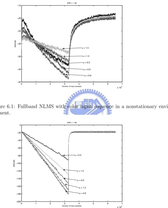
• Figs. 6.1-6.2 illustrate that tracking performance will be not improved the by whitening input signal. These are described in Example 1.

• Figs. 6.3 show two echo paths where the microphone is in different positions of the room and the speaker is fixed. Figs. 6.4-6.6 show three different walk paths that create the time varying channels used for simulation. Figs 6.7-6.12 are comparison of learning curves for the proposed and the conventional tracking methods. These are illustrated in Example 2.

• Figs. 6.13-6.16 are the MSE learning curves of the proposed method with different step size µ. We will see that the initial value of step size does not affect the performance of the proposed method significantly. Figs. 6.17 and 6.18 show the evolution of µ where we see that the evolution trends for different initial values of µ are similar under certain conditions. These are described in Example 3.

• Figs. 6.19-6.22 show the drawback of the proposed method that is unstable under white input signals. These are discuss in Example 4.

Example 1: Convergence rate and tracking performance of full-band NLMS In this example, we see that the ability of whitening input signals of SAF will not improve the performance of tracking ability. Fig. 6.2 and Fig. 6.1 are the MSE learning curves of NLMS adaptive filter with color and white input signals respectively. In the simulations, the echo path is fixed as hecho at first half of iterations, and the echo path is changed at last half of iterations according to

hecho(n + 1) = hecho(n) + c(n), (6.1)

where c(n) is zero-mean white vector and correlation matrix is 0.001I. Although the white input signals has much faster convergence rate than color input signals when channel is static, the tracking performance of the white input signals is not better than that of the color input signals when the echo path is changing. Example 2: MSE comparison between the proposed and the conventional meth-ods

This example presents the performance of the proposed method. The results demonstrate the proposed method outperforms the FSS SAF with AAFCMFB and VSS fullband Adaptive filter. The simulation parameters are as follow: The prototype filter of AAFCMFB has stopband attenuation of 100dB and length of 28. Our simulation environment is as shown in Fig. 2.2 with the room size being 6 × 4 × 2 cube metre. The echo path is obtained by using the Virtual Source Representation with sampling rate being 8192 samples per second [17], see [16]. Figs. 6.3 are two instant echo paths with length 1024. The input signals of the adaptive filters are obtained by passing a white Gaussian signal with zero-mean and unit variance to the single-pole filter with the following transfer function

H(z) = 1

1 − 0.95z−1. (6.2)

According to the simulation in [18], SNR is 30dB or infinite. In our simulation, we set the SNR be 20dB or infinite. Fig. 6.4-6.6 show two different walk paths, where one person takes a microphone and walks around the room with and speaker is fixed. The crystal point is the microphone, and the circle is the speaker. In

0 1 2 3 4 5 6 7 x 104 !45 !40 !35 !30 !25 !20 !15

Number of input samples

MSE(dB) SNR = ! dB µ = 1.5 µ = 1.2 µ = 0.3 µ = 0.9 µ = 0.6

Figure 6.1: Fullband NLMS with color input sequence in a nonstationary envi-ronment. 0 1 2 3 4 5 6 7 x 104 !200 !180 !160 !140 !120 !100 !80 !60 !40 !20 0

Number of input samples

MSE(dB) SNR = ! dB µ = 0.3 µ = 1.5 µ = 0.6 µ = 1.2 µ = 0.9

Figure 6.2: Fullband NLMS with white input sequence in a nonstationary envi-ronment.

Figs. 6.7-6.12, we examine the learning curves for different methods, including AF with NLMS, AF with VSS-NLMS, SAF using AAFCMFB with NLMS and the proposed method, at different SNR values and different walk paths. From above simulations, we observe that the tracking performance of VSS is better than of FSS. Since the colored input signals make the upper bond in equation (A.21) smaller, the performance of VSS fullband AF is almost the same as the FSS fullband AF. This does not occur in the proposed method, because the SAF structure has whiten the input signals of subband filters. In Figs. 6.7 and 6.8, the echo paths are time varying at the beginning. During the time-variant period, the proposed method quickly adapts the step size to a better value which makes the tracking performance up to 5dB lower than the Chang’s method [7] and 9 dB lower than fullband AF respectively. After 4 seconds (32768 samples), the echo paths are fixed. For SNR = 20dB the proposed method has comparable convergence rate as Chang’s method. For noise-free environment, the proposed method has faster convergence rate than Chang’s method. Both of proposed method and Chang’s method have faster convergence rate than fullband AF. In Figs. 6.9 and 6.10, the echo paths are fixed at the beginning. During the time-invariant period, the proposed method has comparable convergence rate as Chang’s method. The echo paths becomes time varying after 4 seconds. During the time-variant period, the proposed method quickly adapts the step size to a better value which makes the tracking performance up to 2 dB lower than the Chang’s method [7] and 4 dB lower than fullband AF respectively for SNR = 20 dB. It makes the tracking performance up to 4 dB lower than the Chang’s method [7] and 7 dB lower than fullband AF respectively for noise-free environment. In Figs. 6.11 and 6.12, the echo path are time varying at the beginning and fixed after 4 seconds. In this case, the proposed method has almost the same performance as Chang’s method when SNR = 20 dB. However, the proposed method outperforms notedly the Chang’s method significantly in tracking performance up to 5dB. Moreover, it has comparable convergence rate with Chang’s method in noise-free environment.

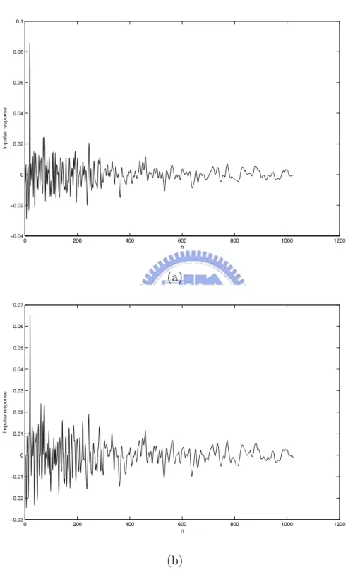
0 200 400 600 800 1000 1200 !0.04 !0.02 0 0.02 0.04 0.06 0.08 0.1 n Impulse response (a) 0 200 400 600 800 1000 1200 !0.03 !0.02 !0.01 0 0.01 0.02 0.03 0.04 0.05 0.06 0.07 n Impulse response (b)

Figure 6.3: Impulse responses of echo paths with different position of room, where the microphone leaves 6 centimeters of loudspeakers in (a) and the microphone leaves 30 centimeters of loudspeakers in (b)

!"#$%"&"'"#$%" !"#$%

'"#$%"& ("#$%"

Figure 6.4: one person stand near the speaker initially, and walks straight with velocity 0.707m/s at first 4 seconds, then stay here for 4 seconds

!"#$%"&"'"#$%" '"#$% ("#$%"&

!"#$%"

Figure 6.5: the person stay near the speaker at first 4 seconds, and walks straight with velocity 0.707m/s for 4 seconds.

!"#$%&' _#"($%'&

(")%&'

Figure 6.6: one person stand near the speaker initially, and walks along the wall with velocity 0.5m/s at first 2 seconds, and then turns right for 2 seconds. Finally, stay here for 4 seconds

0 1 2 3 4 5 6 7 x 104 !34 !32 !30 !28 !26 !24 !22 !20 !18 !16

Number of input samples

MSE(dB) SNR = 20 dB FSS fullband AF µ = 0.4 VSS fullband AF µ_ini = 0.4 " = 0.01 FSS SAF µ = 0.4 VSS SAF µ_ini = 0.4 " = 0.01

Figure 6.7: Learning curves under SNR 20dB when the echo path is according to Fig. 6.4 0 1 2 3 4 5 6 7 x 104 !45 !40 !35 !30 !25 !20 !15

Number of input samples

MSE(dB) SNR = ! dB FSS fullband AF µ = 0.4 VSS fullband AF µ_ini = 0.4 " = 0.01 FSS SAF µ = 0.4 VSS SAF µ_ini = 0.4 " = 0.01

Figure 6.8: Learning curves under noise absent when the echo path is according to Fig. 6.4

0 1 2 3 4 5 6 7 x 104 !32 !30 !28 !26 !24 !22 !20 !18 !16

Number of input samples

MSE(dB) SNR = 20 dB FSS fullband AF µ = 0.4 VSS fullband AF µ_ini = 0.4 " = 0.01 FSS SAF µ = 0.4 VSS SAF µ_ini = 0.4 " = 0.01

Figure 6.9: Learning curves under SNR 20dB when the echo path is according to Fig. 6.5 0 1 2 3 4 5 6 7 x 104 !45 !40 !35 !30 !25 !20 !15

Number of input samples

MSE(dB) SNR = ! dB FSS fullband AF µ = 0.4 VSS fullband AF µini = 0.4 " = 0.01 FSS SAF µ = 0.4 VSS SAF µ_ini = 0.4 " = 0.01

Figure 6.10: Learning curves under noise absent when the echo path is according to Fig. 6.5

0 1 2 3 4 5 6 7 x 104 !32 !30 !28 !26 !24 !22 !20 !18

Number of input samples

MSE(dB) SNR = 20 dB FSS fullband AF µ = 0.4 VSS fullband AF µ_ini = 0.4 " = 0.01 VSS SAF µ_ini = 0.2 " = 0.01 FSS SAF µ = 0.4

Figure 6.11: Learning curves under SNR 20dB when the echo path is according to Fig. 6.6 0 1 2 3 4 5 6 7 x 104 !45 !40 !35 !30 !25 !20 !15

Number of input samples

MSE(dB) SNR = ! dB FSS fullband AF µ = 0.4 VSS fullband AF µ_ini = 0.4 " = 0.01 FSS SAF µ = 0.4 VSS SAF µ_ini = 0.2 " = 0.01

Figure 6.12: Learning curves under noise absent when the echo path is according to Fig. 6.6

Example 3: Sensitivity of initial step size

Figs. 6.13-6.16 show the MSE learning curves of the proposed method with the same initial step size but different ρ. We can observe that the performance of the proposed method is not sensitive to initial value of step size. The step size evolution of the first subband filter in Fig. 6.14 is illustrated in Fig. 6.17 and that in Fig. 6.16 is shown in Fig. 6.18. We observe that the step size evolutions have similar trend and adapt to be close for the following conditions:

• different initial value, • the same walk paths and • the same ρ

Example 4: Drawback of the proposed method

Several evolutions of different step sizes are shown in Figs. 6.19-6.22. The input signals are white in Figs. 6.19-6.20 and color in Figs. 6.21-6.22. The echo path is fixed as hecho at the first half of iterations, and the echo path is changed at the last half of iterations according to (6.1), where c(n) is obtained by passing the zero-mean white vector s(n) into AR process

c(n + 1) = αc(n) + s(n), (6.3)

where α is a scalar. If the input is white, the evolution of step size adapts to the bounded value defined in Equation (A.22) and do not converge to a static value as Figs. 6.21 and 6.22. Then the advantage of VSS is destroyed. We do not have reasonable answer for this phenomenon.

0 1 2 3 4 5 6 7 x 104 !34 !32 !30 !28 !26 !24 !22 !20 !18

Number of input samples

MSE(dB)

SNR = 20 dB

VSS SAF µ_ini = 0.6 " = 0.01

VSS SAF µ_ini = 0.4 " = 0.01 VSS SAF µ_ini = 0.2 " = 0.01

Figure 6.13: Learning curves of proposed method with different initial step size under SNR 20dB when the echo path is according Fig. 6.4

0 1 2 3 4 5 6 7 x 104 !45 !40 !35 !30 !25 !20 !15

Number of input samples

MSE(dB)

SNR = ! dB

VSS SAF µ_ini = 0.2 " = 0.01 VSS SAF µini = 0.4 " = 0.01

VSS SAF µini = 0.6 " = 0.01

Figure 6.14: Learning curves of proposed method with different initial step size under noise absent when the echo path is according Fig. 6.4

0 1 2 3 4 5 6 7 x 104 !32 !30 !28 !26 !24 !22 !20 !18

Number of input samples

MSE(dB)

SNR = 20 dB

VSS SAF µini = 0.2 " = 0.01

VSS SAF µ_ini = 0.4 " = 0.01 VSS SAF µ_ini = 0.6 " = 0.01

Figure 6.15: Learning curves of proposed method with different initial step size under SNR 20dB when the echo path is according Fig. 6.5

0 1 2 3 4 5 6 7 x 104 !45 !40 !35 !30 !25 !20 !15

Number of input samples

MSE(dB)

SNR = ! dB

VSS SAF µ_ini = 0.2 " = 0.01

VSS SAF µ_ini = 0.4 " = 0.01 VSS SAF µ_ini = 0.6 " = 0.01

Figure 6.16: Learning curves of proposed method with different initial step size under noise absent when the echo path is according Fig. 6.5

0 0.5 1 1.5 2 2.5 3 3.5 x 104 0.1 0.2 0.3 0.4 0.5 0.6 0.7 0.8 0.9 1 1.1 n µ µ_ini = 0.2 µini = 0.4 µini = 0.6

Figure 6.17: Evolutions of the step size of Fig. 6.14 with different initial value.

0 0.5 1 1.5 2 2.5 3 3.5 x 104 0.1 0.2 0.3 0.4 0.5 0.6 0.7 0.8 0.9 1 1.1 n µ µ_ini = 0.2 µ_ini = 0.4 µini = 0.6

0 0.5 1 1.5 2 2.5 3 3.5 x 104 0 0.2 0.4 0.6 0.8 1 1.2 1.4 1.6 1.8 2 n µ (n) # = 0.76 # = 0.3 # = 0 # = !0.76 # = 0

Figure 6.19: Evolutions of the step size with white input in different α = −0.76, −0.3, 0, 0.3, 0.76, and the initial value of step size is 0.4.

0 0.5 1 1.5 2 2.5 3 3.5 x 104 0 0.2 0.4 0.6 0.8 1 1.2 1.4 1.6 1.8 2 n µ (n) # = !0.3 # = !0.76 # = 0 # = 0.3 # = 0.76

Figure 6.20: Evolutions of the step size with white input in different α = −0.76, −0.3, 0, 0.3, 0.76, and the initial value of step size is 1.4.

0 0.5 1 1.5 2 2.5 3 3.5 x 104 0 0.2 0.4 0.6 0.8 1 1.2 1.4 1.6 1.8 2 # = 0 # = !0.76 # = !0.3

Figure 6.21: Evolutions of the step size with color input in different α = −0.76, −0.3, 0, 0.3, 0.76, and the initial value of step size is 0.4.

0 0.5 1 1.5 2 2.5 3 3.5 x 104 0 0.2 0.4 0.6 0.8 1 1.2 1.4 1.6 1.8 2 # = 0.76 # = 0.3 # = 0 # = !0.76 # = !0.3

Figure 6.22: Evolutions of the step size with color input in different α = −0.76, −0.3, 0, 0.3, 0.76, and the initial value of step size is 1.4.

Chapter 7

Conclusion and Future work

In this thesis, we proposed a method to improve the tracking ability of SAF using AAFCMFB with variable step size. The proposed method can improve tracking performance of time varying echo path up to 9 dB for noise-free case and 5 dB for SNR = 20 dB as well as it keeps fast convergence rate. By using the structure of subband adaptive filters, the proposed method also requires less computational complexity which is at most 68% of the complexity of fullband adaptive filter with VSS-NLMS. Moreover, the proposed method is insensitive to initial value of step size. This is shown in Chapter 6 that different initial values of step size leads to very similar steady state performance. Thus all we need to do is choosing a suitable ρ, which is a parameter for step-size adaptation. A rule of thumb for ρ is ranged from 0.01 to 0.001, which is a loose rule. The future work is described below: For a more practical situation, we can consider the correlation for time-variant echo path and add this factor into our current derivation for optimal variable step size. In this case, the corresponding performance may also need to be re-evaluated accordingly.

Appendix A

The Range of Step Size for

Stability

In the following, we discuss the stability of convergency. Most derivation of this chapter can be see in [15], which is presented a condition of step size in LMS algorithm. However, this condition is not reasonable of the environment which has relative white input signal. Thus we need to make some modifications to get a reliable condition on step size. To achieve this goal, we derive the correlation matrix of weight-error vector with fixed step size first

E2vn+1vTn+1 3 = E(!vn+ x_n #xn#2µe(n) − cn " ! vT n + µe(n) xT n #xn#2 − c T n "* = E2vnvnT 3 + E(xn µ2_e(n)2 #xn#4 x T n * + E2cncTn 3 +E(xn_#vµe(n) n#2v T n * + E(vn_#xµe(n) n#2x T n * = E2vnvnT 3 − µ@E(xnxTnvnvTn #xn#2 * + E(vnvTnxnxTn #xn#2 *A +µ2_E > xn( ν2(n)+vT nxnxTnvn) #xn#4 x T n ? + E2cncTn 3 . (A.1)

Let ˜vn = Qnvn, ˜xn = Qnxn and ˜cn = Qncn, where Qn is obtained by (4.11). Then (A.1) becomes

E2˜vn+1˜vTn+1 3 = E2˜vn˜vnT 3 − µ@E(˜xn˜xTn˜vn˜vTn #˜x_n#2 * + E(˜vnv˜Tn˜xnx˜Tn #˜x_n#2 *A +µ2_E > ˜ xn( ν2_(n)+˜vT n˜xn˜xTn˜vn) #˜x_n#4 ˜x T n ? + E2˜cn˜cTn 3 = E2˜vn˜vnT 3 − _E[#˜xµ_n#2] 4 E2˜xn˜xTnv˜nv˜Tn 3 + E2˜vn˜vTn˜xn˜xTn 35 +_#˜xµ2 n#4E 2 ˜ xn / ν2_{(n) + ˜x}T n˜vn˜vnT˜xn 0 ˜ xT n 3 + E2˜cn˜cTn 3 (A.2) where E2x˜nx˜Tn˜vn˜vTn˜xn˜xTn 3 = <_N−1 & p=0 N_&−1 q=0 E [˜xn,ıx˜n,pE [˜vn,pv˜n,q] ˜xn,qx˜n,] = ı   0≤ı,≤N −1 = <_N−1 & p=0 N_&−1 q=0 E [˜xn,ıx˜n,p] E [˜vn,pv˜n,q] E [˜xn,qx˜n,] = ı + <_N−1 & p=0 N_&−1 q=0 E [˜xn,ıx˜n,q] E [˜vn,pv˜n,q] E [˜xn,px˜n,] = ı + <_N−1 & p=0 N_&−1 q=0 E [˜xn,ıx˜n,] E [˜vn,pv˜n,p] E [˜xn,px˜n,q] = ı   0≤ı,≤N −1 = (E [˜xn,ıx˜n,ı] E [˜vn,ıv˜n,] E [˜xn,x˜n,])_ı + (E [˜xn,ıx˜n,ı] E [˜vn,ıv˜n,] E [˜xn,x˜n,])_ı + <_N−1 & p=0 E [˜xn,ıx˜n,] E 2 ˜ v2 n,p 3 E2x˜2 n,p 3= ı   0≤ı,≤N −1 = 2ΛnE 2 ˜ vn˜vnT 3 Λn+ Λntr 4 ΛnE 2 ˜ vnv˜Tn 35 . (A.3)

Then E2v˜n+1˜vn+1T 3 = E2v˜nv˜Tn 3 −_E[#˜xµ_n#2] 4 ΛnE 2 ˜ vn˜vTn 3 + E2v˜nv˜Tn 3 Λn 5 + µ2 E[#˜x_n#4] 2 2ΛnE 2 ˜ vnv˜Tn 3 Λn+ Λntr 4 ΛnE 2 ˜ vn˜vTn 353 + µ2σν2 E[#˜x_n#4]Λn+ σ 2 cIN (A.4)

The matrix form (A.4) can be decomposed into the following scalar equations:

˜ Vı(n + 1) =      ! 1 − 2λıµ N σ2 x + 2λ2 ıµ2 N2_σ4 x " ˜ Vı(n) + λıµ 2 N2_σ4 x N−1_& !=0 λ!V˜!!+λıµ 2_σ2 ν N2_σ4 x + σ 2 c , ı =  ! 1 − (λı+λı)µ N σ2 x + 2λıλµ2 N2_σ4 x " ˜ Vı(n) , ı %= , (A.5) where ˜ Vı(n) = / E2˜vn˜vTn 30 ı. (A.6)

It is easy to see that V2

ı ≤ VııV, so we can just consider the diagonal term. Let bn= ( ˜ V00V˜11. . . ˜VN−1N −1 * . Then bn+1= Fbn+ µ2_σ2 ν N2_σ4 x λ_{+ σc}2ı_{, (A.7)} where F =     1 −2λ0µ N σ2 x + 2λ2 0µ2 N2_σ4 x . .. 1 − 2λN −1µ N σ2 x + 2λ2 N −1µ2 N2_σ4 x     + µ2 N2_σ4 x λλT_{, (A.8)} λ_{= [λ0λ1. . . λN − 1]}T _(A.9) and ı_{= [11 . . . 1]}T_{. (A.10)}

According to linear algebra, bn will converge if and only if all eigenvalues of F are within the unit circle. To find the eigenvalues of matrix F, we have to find the solution of the following equation in α

where det[·] denote the determinant. We also know that F − αIN = diag {f0. . . fN−1} + µ 2 N2_σ4 x λλT = diag@√f0. . . Q fN−1 A ( IN +µ 2λ#_λ#T N2_σ4 x * diag@√f0. . . Q fN−1 A , (A.12) where f! = 1 − 2λ!µ Nσ2 x + 2λ 2 !µ2 N2_σ4 x − α (A.13) and λ" _{= diag} # 1 √ f0 . . .Q1 fN−1 R λ_{. (A.14)}

Since λ"λ"T _{can be decomposed as}

λ"λ"T _{= L}T        N−1_& !=0 λ2_$ f$ 0 . .. 0        L. (A.15) Then we have det [F − αI]

= det [diag {f0. . . fN−1}] det ( IN +µ 2λ#_λ#T N2_σ4 x * = >_N−1 S !=0 f! ? > 1 + N_&−1 !=0 µ2_λ2 $ f$N2σ4x ? (A.16)

Since the common denominator of the sum of second term is the first term in (A.16), we needs only to consider the second term.

f (α) = 1 + N_%−1 !=0 µ2_λ2 ! (f" !− α)N2σx4 , (A.17) where f" ! = 1 − 2λ$µ N σ2 x + 2λ2 $µ2 N2_σ4

x. There is a example of f (α) with N = 5 in Fig. A.1

!"#$ !"#% !"#& !"#' !"#( !"#) !"#* !"## !"#+ !"+ !"+$ !"+% !"+& !"+' !"+( !"+) !"+* !"+# !"++ $ ,( ,' ,& ,% ,$ $ % & ' (

Figure A.1: The graph of f (α) vs. α. The 5 circles denote 5 zeros of f (α) and the dash lines are asymptotes. x is α, y is f (α)

only if f (1) > 0, i.e. N_%−1 !=0 µλ! Nσ2 x− µλ! < 2. (A.18)

According to [15], the condition of step size µ is given by 0 < µ < 2

3, (A.19)

whose upperbound is too small for the environment which has relative white input. Thus we derived another condition of step size µ. Since

N−1 % !=0 µλ! Nσ2 x− µλ! < N µλmax Nσ2 x− µλmax , (A.20)

where λmax = max {λ!} < _µ2. Then the range of µ for stability is given by 0 < µ < 2σ 2 x λmax . (A.21) Thus If 2σ2x λmax > 2

3, and Then the upperbound of step size is 2σ2

x

λmax, and vice versa.

If the eigenvalue spread of input vector is relative small, we have

Appendix B

Mean Square Deviation

Due to the underlying idea of NLMS is that the weight vector of an adaptive filter should be changed in a minimal manner, subject to a constraint imposed one the update tap-weight vector, MSD(Mean Square Deviation) is an important performance to the stability analysis of the NLMS filter [2], which is a statical performance without considering output noise(MSE is considering output noise) and directly presents the mismatch of weight vector. Let us evaluate the MSD. According to (4.9), we have E2vT n+1vn+1 3 = E((vT n + e(n)µ(n) xT_n #xn#2 − c T n)(vn+ x_n #xn#2e(n)µ(n) − cn) * = E2vT nvn 3 + E(e(n)2_µ(n)2 xTnxn #xn#4 * + E2cT ncn 3 +E(e(n)µ(n)xTnvn #xn#2 * + E(vnTxn #xn#2e(n)µ(n) * . (B.1) According to (4.1) and (4.7), we obtain

e(n) = ν(n) − vT

nxn. (B.2)

Substituting (B.2) into (B.1), and assuming that µ(n) is independent to xn, vn and ν(n). Then we have

E2vT n+1vn+1 3 = E2vT nvn 3 − 2E(µ(n)vTnxnxTnvn #xn#2 * + E(µ(n)2 vTnxnxTnvn+ν(n)2 #xn#2 * +E2cT ncn 3 . (B.3)