正交分頻多工存取下載系統在非完全通道資訊下之資源分配及中繼器選取

(1)

國立交通大學

電信工程研究所

碩士論文

正交分頻多工存取下載系統在非完全通道資訊下之

資源分配及中繼器選取

Downlink Resource Allocation and Relay Selection

for OFDMA Networks With Imperfect Channel

Information

研究生：王俊鋐

指導教授：蘇育德博士

(2)

正交分頻多工存取下載系統在

非完全通道資訊下之資源分配及中繼器選取

Downlink Resource Allocation and Relay Selection

for OFDMA Networks With Imperfect Channel Information

研究生：王俊鋐 Student：Jiun-Hung Wang

指導教授：蘇育德博士 Advisor：Dr. Yu T. Su

國立交通大學

電信工程研究所

碩士論文

A Thesis

Submitted to Institute of Communications Engineering College of Electrical and Computer Engineering

National Chiao Tung University in Partial Fulfillment of the Requirements

for the Degree of Master of Science

in Communications Engineering August 2011

Hsinchu, Taiwan, Republic of China

(3)

正交分頻多工存取下載系統在非完全通道

資訊下之資源分配及中繼器選取

研究生：王俊鋐指導教授：蘇育德博士

國立交通大學電信工程研究所碩士班

中文摘要

正交分頻多工存取(OFDMA)系統可以利用簡單的通道等化器來有效

的避免頻率選擇性衰減並使用最小（Nyquist）次載波距（subcarrier spacing）

來提高頻譜效能。這種多工技術也容許很有彈性的資源分配，以充分利用

不同用戶的通道狀況，一則可滿足個別用戶傳送速率的要求，另則可最大

化整個系統的通道容量。此外，由於電磁信號傳播的統計特性，蜂巢式行

動通訊系統之收訊強度無法定量保證，其中難免有部分用戶收訊品質不

佳。一個經濟有效的解決方案便是中繼站的設立，適當的佈建中繼站不但

有助於提升其信號品質，並可擴增基地台的覆蓋範圍與容量。

本論文主要在研究有多座中繼站的 OFDMA 下鏈系統之資源分配及中

繼站選取的問題。我們同時考慮傳送（基地台）與接收（用戶）端皆使用

單一天線(SISO)以及兩端皆有多根天線(MIMO)兩種架構，而下傳時雖有多

個中繼站可以挑選，但各通道狀況的資訊卻有不確定性；亦即，基地台只

有通道狀況的估計值以及誤差機率分佈。我們使用在此不確定情況下的通

道容量下限來作為系統效能的評估標準。對上述 SISO 與 MIMO 兩種架構

下，我們都推導出傳送端與中繼站的最佳功率比來達到最大的通道容量下

(4)

ii

限。根據這個功率比我們分別提出了幾近最佳的次載波及其能量（功率）

分配的演算法。我們的演算法複雜度不高，電腦模擬結果也顯示它能兼顧

個別用戶的公平性，滿足其傳送速率要求也可以令系統的整體傳送速率達

到最大值。

(5)

Downlink Resource Allocation and Relay Selection

for OFDMA Networks With Imperfect Channel

Information

Student : Jiun-Hung Wang Advisor : Yu T. Su Institute of Communications Engineering

National Chiao Tung University Abstract

The Orthogonal Frequency Division Multiple Access (OFDMA) scheme is an effi-cient anti-fading transmission scheme which renders high spectral efficiency and simple channel equalization. It also allows flexible resource allocation (RA) to meet various user requirements and achieve maximum network capacity. With the help of relays, link quality at cell edge can be improved and both network capacity and the coverage area can therefore be improved.

In this thesis, we consider the problem of RA and relay selection for downlink trans-mission in both single-input single-output (SISO) and multiple-input multiple-output (MIMO) OFDMA based cellular networks. We assume the availability of multiple co-operative relay stations but not the perfect channel state information (CSI). Instead, the base station knows only the estimated channel (link) gain and the associated error distribution. We use a tight capacity lower bound (CLB) for a link with imperfect CSI as the performance metric. In SISO networks, we derive the optimal source and relay power allocation ratio that maximizes the CLB of a cascaded source-relay-destination link. Based on this optimal power ratio, we propose a simple suboptimal algorithm that assigns power, subcarriers and cooperative relays to each serving mobile station. We

(6)

then derive the optimal power ratio for MIMO networks. Using the proposed subcar-rier assignment algorithm for SISO network, we present the optimal and a suboptimal power allocation schemes. To reduce the computation complexity, we derive a near-optimal power ratio, assuming both source-to-relay and relay-to-destination links have the same rank. Simulation results show that our algorithm not only meets the users’ rate constraints with very high probabilities but yields an excellent sum rate (CLB) performance.

(7)

誌謝

對於論文得以順利完成，首先感謝我的指導教授蘇育德博士。老師

除了在專業上面的教導之外，做人處世的態度也令我受益匪淺。另外也感

謝口試委員蘇賜麟教授、林茂昭教授、呂忠津教授以及吳卓諭教授給予的

寶貴意見，以補足這分論文的缺失與不足之處。而在實驗室方面，也特別

感謝林淵斌學長、劉人仰學長、張致遠學長、劉彥成學長以及其他學長姐、

同學和學弟妹在這兩年內的不論是研究上或上生活上的幫忙與鼓勵。

最後，感謝一路上不斷支持我的家人，他們的關心與鼓勵帶給了我無

形的動力，僅獻上此論文，以代表我最深的敬意。

(8)

List of Figures

3.1 SISO system model . . . 8 3.2 The probability density function of the user location distribution; r0 = 150

m. . . 14 3.3 The user location distribution; r0 = 150 m. . . 15

3.4 Sum rate v.s. user rate constraint; 8 DNs, 3 RNs and 32 subcarriers with

PT = 3.2. . . . 16

3.5 Rate failure probability v.s. user rate constraint;8 DNs, 3 RNs and 32 subcarriers with PT = 3.2. . . . 17

3.6 Sum rate v.s. user number; 3 relay nodes and 32 subcarriers with PT = 3.2

and the minimum user rate requirement is 48 bits/2 OFDM symbols. . . 18 3.7 Rate failure probability v.s. user number; 3 relay nodes and 32 subcarriers

with PT = 3.2 and the minimum user rate requirement is 48 bits/2 OFDM

symbols. . . 19 3.8 Average achievable rate ratio for the rate failure event v.s. user number;

3 relay nodes and 32 subcarriers with PT = 3.2 and the minimum user

rate requirement is 48 bits/2 OFDM symbols. . . 19 3.9 Load balance probability v.s. user number; 3 relay nodes and 32

subcar-riers with PT = 3.2 and the minimum user rate requirement is 48 bits/2

OFDM symbols. . . 20 3.10 Sum rate v.s. user rate constraint; 8 DNs, 3 RNs and 128 subcarriers

(11)

3.11 Rate failure probability v.s. user rate constraint;8 DNs, 3 RNs and 128 subcarriers with PT = 12.8. . . . 21

3.12 Sum rate v.s. user number; 3 relay nodes and 128 subcarriers with PT =

12.8 and the minimum user rate requirement is 48 bits/2 OFDM symbols. 21 3.13 Rate failure probability v.s. user number; 3 relay nodes and 128

subcar-riers with PT = 12.8 and the minimum user rate requirement is 48 bits/2

OFDM symbols. . . 22 4.1 MIMO system model . . . 23 4.2 One cooperative path in Fig.4.1 . . . 24 4.3 Sum rate v.s. user rate constraint; 8 DNs, 4 RNs and 32 subcarriers . . . 40 4.4 Rate failure probability v.s. user rate constraint;8 DNs, 4 RNs and 32

subcarriers. . . 41 4.5 Sum rate v.s. user number; 4 relay nodes and 32 subcarriers and the

minimum user rate requirement is 30 bits/2 OFDM symbols. . . 41 4.6 Rate failure probability v.s. user number; 4 relay nodes and 32 subcarriers

and the minimum user rate requirement is 30 bits/2 OFDM symbols. . . 42 4.7 Sum rate v.s. user rate constraint; 8 DNs, 4 RNs and 32 subcarriers . . . 42 4.8 Rate failure probability v.s. user rate constraint;8 DNs, 4 RNs and 32

and the minimum user rate requirement is 30 bits/2 OFDM symbols. . . 44 4.11 Sum rate v.s. user rate constraint; 8 DNs, 4 RNs and 32 subcarriers. . . 44 4.12 Sum rate v.s. user number; 4 relay nodes and 32 subcarriers and the

minimum user rate requirement is 30 bits/2 OFDM symbols. . . 45 4.13 Sum rate v.s. user rate constraint; 8 DNs, 4 RNs and 32 subcarriers . . . 50

(12)

4.14 Rate failure probability v.s. user rate constraint;8 DNs, 4 RNs and 32 subcarriers. . . 50 4.15 Sum rate v.s. user number; 4 relay nodes and 32 subcarriers and the

and the minimum user rate requirement is 30 bits/2 OFDM symbols. . . 51 4.17 Sum rate v.s. user rate constraint; 8 DNs, 4 RNs and 32 subcarriers . . . 52 4.18 Rate failure probability v.s. user rate constraint;8 DNs, 4 RNs and 32

and the minimum user rate requirement is 30 bits/2 OFDM symbols. . . 53 4.21 Sum rate v.s. user rate constraint; 8 DNs, 4 RNs and 32 subcarriers. . . 54 4.22 Sum rate v.s. user number; 4 relay nodes and 32 subcarriers and the

minimum user rate requirement is 30 bits/2 OFDM symbols. . . 54 4.23 Rate per subcarrier v.s. edge user SNR; 1 DNs, 4 RNs and 1 subcarriers. 55 4.24 Rate per subcarrier(normalized to optimal) v.s. edge user SNR; 1 DNs,

(13)

List of Tables

3.1 Subcarrier assignment algorithm. . . 13 4.1 Proposed optimal power allocation. . . 56

(14)

Chapter 1 Introduction

The Orthogonal Frequency Division Multiple Access (OFDMA) scheme enjoys the advantages of an OFDM based transmission system, i.e., high spectral efficiency, simple and robust equalization against frequency selective fading; it also offers flexibility in radio resource allocation for meeting various rate requirements. Due to OFDMA transmits a wide band signal on multiple orthogonal subcarriers, in which the channel condition of one subcarrier is independent of one another, which means a subcarrier in deep fading for one user may have good condition for another user. Thus, by proper scheduling and resource block assignment, OFDMA can exploit multi-user diversity [1] in a time-varying frequency-selective fading channel. As a result, the OFDMA scheme has been selected as the air interface standard by two major 4G campaigns, namely, the IEEE802.16m and 3GPP’s LTE-A downlink.

Recent researches have found that, a base station (BS) can cooperate with relay sta-tions using a Time Division Duplex (TDD) based Decode-and-Forward (DF) or Amplify-and-forward (AF) scheme to enhance the network capacity. In a typical two-phase coop-erative system, the transmitter sends its signal to a relay node (RN) and the destination node (DN) in the first half of a transmission frame and the relay then sends the re-generated signal to the destination in the second half [3]. By combining the two copies received in both phases, the DN increases the link’s capacity.

(15)

To maximize the sum rate, a BS in a relay based cooperative network must dy-namically allocate its resources, namely, power, subcarriers and cooperative RNs to various DNs (i.e., mobile stations) according to the conditions of the BS-DN, BS-RN, and RN-DN links. The problem of resource allocation in either conventional OFDMA or relay-aided OFDMA systems has been intensively studied [4], [5]. But in these works, a common assumption is that the channel state information (CSI)–the gains of all links–of the system is perfectly known by the BS.

However, the channel information is estimated by dividing the demodulated pilot pattern with the known symbol. Due to the additive noise in demodulating the received preamble, the channel estimation error can be assumed as a gaussian random variable [11]. Moreover, due to feedback delays, channel estimation errors in transmitter are unavoidable. For the feedback delay error, since the channel is modeled as a Gaussian random process, the channel gain and its delayed version then can be a jointly Gaussian [10]. Thus, perfect CSI assumption leads to underuse or overuse of component links and are likely (especially in relay-aided links) to results in transmission outages [12]. [13] considered optimal resource allocation for maximizing the ergodic sum rate of an OFDMA system with imperfect CSI. A suboptimal algorithm for goodput maximization was given in [14]. To our knowledge, [15] is the only work which investigates the issue of joint relay selection and resource allocation in a cooperative relay network with imperfect CSI. However, the authors used a mean rate to characterize the CSI uncertainty which may lead to different interpretations.

In this thesis, we consider a problem similar to that studied in [14] under a different performance metric. As the channel capacity in the presence of imperfect CSI is not known [16], we use a tight capacity lower bound as the performance metric and derive the corresponding optimal source (BS) and RN power ratio if a given RN is to be used for relaying the source signal to a DN. We then present a low-complexity resource allocation scheme with an aim to not only maximize the total sum rate (lower bound) but also

(16)

meet the users’ (DNs’) rate and power constraints. The scheme includes link (direct link only or a relay is needed) selection, subcarriers assignments(SA) and power allocation (PA).

This thesis is organized as follows: In following chapter, we describe the system model and related assumptions for the problem of concern. In chapter 3, we proposed algorithms to solve the problem we face. Moreover, we extend the resource allocation problem to the case for multiple-input and multiple-output(MIMO) case in chapter 4. Finally, we conclude our work in chapter 5.

(17)

Chapter 2 Relay System and Cooperative

Transmission

2.1 Relay Networks

In a wireless communication system, one of the most important problems is the fading effect. While in recent years, cooperative communications have been used to exploit the spatial diversity in multiuser wireless systems without the need of multiple antennas at each node, which is not practical to employee in a mobile station(MS) due to the receive and transmit antennas should be separated far enough. Moreover, the term cooperative communications typically means a system where users share and coordinate their resources to enhance the transmission quality.

In a basic cooperative communication system, it consists a source node, a relay node and a destination node. Depending on the condition of the component links between source node and relay node, relay node and destination node, and source node and des-tination node, the source node can choose to whether use the relay or not. If the source uses relaying, destination combines the two copies from source node and relay node, the cooperative diversity can be utilized. Futhermore, for a much general cooperative communication system, there are multiple source nodes, relay nodes, and destination nodes. Thus, by opting to transmit a data stream to the appropriate destination node

(18)

from a appropriate relay node, the source node gains the multiuser diversity.

2.2 Relay Strategies

Many cooperation techniques have been proposed based on the concept of relaying [2], the most commonly used strategies in these methods are decode-and- forward (DF) and amplify-and-forward (AF). For a two-hop relaying we’ll use in our scenario, the source node broadcasts its message to both the relay node and the destination. If the relay node employs the DF scheme, it will decode and regenerate a new message to the destination in second phase. At the destination, it employs a maximum-ratio-combining detector to the signals from both the source and the relay paths. Otherwise, if the AF scheme is used, the relay node just simply amplify the received signal and forwards it direcatly to the destination. No decoding of the message is needed in AF scheme.

Moreover, in [6], it compares the performance of DF with the performance of AF scheme. It shows that the distance between the relay node, the source node, and the destination node is the most important point to influence the performance of each relay-ing scheme. When the distance between relay node and source node is lower than the distance between relay node and destination node, the relay node has a higher received signal-to-noise ratio(SNR). Thus, DF is a better scheme for the relay node to employ. Otherwise, when the distance between relay node and source node is higher than the dis-tance between relay node and destination node, the relay node has a higher probability of the decoding error. Then, we’ll choose the AF scheme for relaying.

However, the reliability of interuser channels also relate to the performance of relay cooperation. In the DF scheme, the relay node node retransmits the signal from the source only if the signal is well decoded. Similarly, for the AF scheme, due to both the signal and noise are amplified by relay node, if the quality of the source-relay link is bad, the performance at the destination node will decrease. Therefore, we need to decide whether to use the relays or not according to the source-relay channel.

(19)

2.3 Capacity of Cooperative Transmissions

In [7], the capacity of basic cooperative transmissions has been introduced. If we denote Xs, Xr, Yr and Yd the transmitted signals from source and relay, the received

signal at relay and destination, respectively. The capacity of a relay channel with channel transition probability p(yr, yd|xs, xr) is

C ≤ sup

p(xs,xr)

min {I(Xs, Xr; Yd), I(Xs; Yr, Yd|Xr)} (2.1)

where the sup is over all joint distributions p(xs, xr).

Under the derived capacity (2.1), if we denote SNRSR, SNRRD and SNRSD the

SNR of source-relay, relay-destination and source-destination path, the capacity of a single user, single relay and single destination cooperative communication system can be formulated as

C ≤ min {log2(1 + SN RSR), log2(1 + SNRSD+ SNRRD)} (2.2)

where the second term is due to the maximum-ratio-combining detector at the destina-tion node.

(20)

Chapter 3 Downlink Resource/Relay

Allocation for SISO OFDMA

Networks

This chapter considers the scenario for a downlink single-input single-output OFDMA system as shown below. We represent resource allocation schemes that maximize the total capacity with each user’s minimum rate constraint and the overall total power constraint while facing the channel estimated errors. By taking the channel estimated errors into account, we derive a tight capacity lower bound as the performance matrix. Then we propose a simple suboptimal algorithm that assigns power, subcarriers and cooperative relays to each mobile station.

3.1 System Model and Assumptions

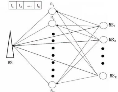
We consider the downlink of an N-subcarrier OFDMA cooperative network which contains a BS, M fixed relay nodes, and K MS’s equipped with one antenna and ran-domly distributed within a cell. Similar to the conventional relay-based cooperative communication systems, we assume a two-phase (time-slot) transmission scheme with perfect timing synchronization among all network users. Each subcarrier suffers from slow flat Rayleigh fading and there is no change of the channel state during a two-phase period. A data stream from a source user must be carried by the same subcarrier no

(21)

Figure 3.1: SISO system model

matter it is transmitted by a source node or a relay node. As mentioned in the previous section, our protocol offers both relay-aided (RA) and non-relay-aided (NRA) modes. We consider the decode-and-forward (DF) cooperative relay scheme only and assume that the maximum-ratio-combining detector is employed by the destination (user) node, assuming perfect decoding at the relays. Although the system model presented below describes a downlink setup, it can be easily converted into an uplink scenario with all the results obtained remain valid.

We assume the mobile user obtains the channel information by MMSE estimator and the feedback of the estimate is instantaneous and perfect to the BS. We also assume that the phase of the channel gain can be perfectly acquired while having channel estimation error which pertains to the amplitude of the correct channel gain. As a result, the same channel information about the channel gain with an estimation error is available simul-taneously to both the transmitter and the receiver. Based on the imperfect CSI from all users and the minimum rate requirement of each MS, the BS acts as a central control device to carry out all resource allocation related operations which include collecting link information, appropriating resources, and informing MS’ about their assigned resources.

(22)

3.2 Achievable rates for RA and NRA modes

For the source-to-destination link, the matched filter output at the destination node can be expressed as

r = (bh + eh)x + w (3.1) where bh denotes the estimated complex channel gain, eh is the estimation error which

can be modelled as a zero-mean complex Gaussian random variable with variance σ2

h, w

is the complex white Gaussian noise with variance σ2

n.

Although a closed-form expression for the capacity of the above link is not known, a tight lower bound CLB (in bits/sec/Hz) is given by [16]

CLB = log2 " 1 + P |bh|2 P σ2 h+ σn2 # (3.2) where P = Ekxk2_{. For brevity, we will refer to link capacity and its lower bound}

interchangeably in the subsequence discourse unless there is danger of ambiguity. For the same reason, we denote by hSD(k, n) the estimated (component) link gain between

the BS and the kth MS, by hRD(k, m, n) that between the mth relay and the kth MS,

and by hSR(m, n) that between BS and relay m, all on subcarrier n. The corresponding

transmit powers are denoted by pS(n, k), pRD(k, m, n), pSR(m, n).

Using the above notations, we express the capacity (lower bound) of a basic cooper-ative network with imperfect CSI as

(23)

and αm, αk, αk,m are the path losses of source to relay (SR), source to destination (SD),

and relay to destination (RD) links, respectively. For simplicity, we will henceforth denote hSR(m, n) by hSR, hSD(k, n) by hSD, and hRD(k, m, n) by hRD. For a given sum

power, P = pSR(m, n) + pRD(k, m, n), the optimal power distribution ratio Γ(k, m, n, P )

that maximizes the capacity is given by

Γ(k, m, n, P ) = pRD(k, m, n) pSR(m, n) = (x1) 1 3 + (x 2) 1 3 +a 3 (3.5) where x1 = 1₂ µ 2a3 27 +ab3 + c + q¡_2a3 27 + ab3 + c ¢2 − 4(3b+a₇₂₉2)3 ¶ , x2 = 1₂ µ 2a3 27 +ab3 + c − q¡_2a3 27 + ab3 + c ¢2 − 4(3b+a₇₂₉2)3 ¶ , and a = αk,mσ2n|hRD|2, b = P [αmαk,mσ2hσ2n|hSR|2− αkαk,mσh2σ2n|hSD|2−αk,mαmσ2hσ2n|hRD|2 − αk,mαkσh2σn2|hRD|2] + [αmσn4|hSR|2− αkσn4|hSD|2 − 2αk,mσ4n|hRD|2], c = P2_σ4 hαmαkαk,m[|hSR|2− |hSD|2− |hRD|2] +P σ2 hσn2[αmαk|hSR|2+ αmαk,m|hSR|2 −αkαm|hSD|2− αkαk,m|hSD|2−αk,mαm|hRD|2− αk,mαk|hRD|2] +σ4 n[2αm|hSR|2− 2αk|hSD|2− αk,m|hRD|2], d = P σ2 hσ2n[αmαk|hSR|2− αkαm|h2SD] + σn4[αm|hSR|2− αk|hSD|2]

The corresponding maximum achievable rate is

rm(k, n, P ) = log2 " 1 + P 1+Γ(k,m,n,P )αm|hSR(m, n)|2 P 1+Γ(k,m,n,P )αmσh2 + σn2 # (3.6) Since in NRA mode, we allow the source to be active for both phases, a fair comparison on the achievable rate should be measured with respect to the total consumed energy. The resulting link capacity over two OFDM symbols is

rD(k, n, P ) = 2 log2 " 1 + P 2αk|hSD(k, n)|2 P 2αkσ2h+ σn2 # (3.7)

(24)

3.3 Problem Formulation

To begin with, we define ρ(k,n,m) as the subcarrier assignment and link selection

indicator so that ρ(k,n,m) = 1 and m > 0 indicates subcarrier n is allocated to user k who

options for RA mode using relay node m while m = 0 indicates the user options for the NRA mode. Otherwise, user k does not have access to subcarrier n over the mth link. Suppose the available total transmission power is PT, then the problem of maximizing

the total system rate under the users’ rate constraints is equivalent to max K X k=1 Rk = max K X k=1 N X n=1 M X m=0 ρ(n,k,m)rm(k, n, pm(k, n)) subject to Rk ≥ Rk,min ∀k K X k=1 M X m=0 ρ(n,k,m) ≤ 1 ∀n ρ(n,k,m)∈ {0, 1} ∀ n, k, m N X n=1 K X k=1 M X m=0 ρ(n,k,m)pm(k, n) ≤ PT (3.8)

where Rk and Rk,min are the achievable rate and the minimum rate requirement for

user k, and r0(k, n, P ) = rD(k, n, P ). The above formulation is an NP-hard mixed

integer programming problem. Instead of finding the optimal solution, we propose a low-complexity suboptimal algorithm in the following section.

3.4 Proposed Resource Allocation Schemes

We decompose the task of joint subcarrier/power assignment and the corresponding link selection into a three-stage process which can be described by ρ(n,k,m) = δ(n,k)βm(n, k),

where δ(n,k) and βm(n, k) represent the subcarrier assignment and link selection

opera-tions, respectively, i.e., δ(n,k) = 1 implies that subcarrier n is allocated to user k, and

βm(n, k) = 1 means user k sends its data over subcarrier n with the help of relay m.

(25)

The original problem is thus divided into three subproblems: P1–link selection sub-problem for deciding {βm(n, k)}, P2–subcarrier assignment for deciding {δ(n,k)}, and

P3–power allocation. In the first stage, we select for each DN the best link among (M + 1) candidate relay links. Based on the selected relay links, the BS then allocate subcarriers to each DN according to its link gain and minimum rate requirement. The BS tries to maximize the user diversity gain under the minimum rate constraints. In the third stage, we proceed to allocate power by taking into account the channel estimation error.

3.4.1 Relaying/Direct link selection rule

Since the optimal relay/BS power ratio Γ depends on the available transmit power and the final power allocation is still unknown, we assume a fair power distribution PT

N

for all DNs. We then determine if a relay is needed for user k if subcarrier n is available by

m∗ _{= arg max}

0≤m≤Mrm(k, n, PT/N) (3.9)

When m∗ _{= 0, DN k should use only the direct link if it was given subcarrier n. We}

then set βm∗(n, k) = 1 and β_m(n, k) = 0, for 0 ≤ m ≤ M, m 6= m∗.

3.4.2 Subcarrier assignment

Many suboptimal subcarrier assignment algorithm has been proposed but most of them seldom consider the user rate constraint in this step. They usually assign a subcar-rier to the DN who has the best channel gain on this subcarsubcar-rier [8]. Instead of choosing the user k∗_{having the largest weighted rate [9], w}

k×r(k, n) with wk def

= Rk,min−Rk

Rk,min and Rk

being the current rate for DN k, we choose (k∗_{, n}∗_{) which gives the maximum weighted}

rate over all users and unassigned subcarriers. The process repeats until either all the rate requirements are met or all subcarriers are assigned. For the former case, we assign each of the remaining subcarriers to the one having best rate on it. If the latter case

(26)

occurs, we need a rate-balancing step after power allocation. The complete subcarrier assignment algorithm is summarized in Table (3.1).

Given r(k, n) and δ(n,k) = 0, for 1 ≤ k ≤ K, 1 ≤ n ≤ N

Set U = {1, 2, ....N} , and rk= 0 ∀ k while (|U| ≥ 1) Wk= (Rk,min− Rk)/Rk,min ∀ k if (max1≤k≤KWk> 0) (n∗_{, k}∗_{)= arg max} n∈U ,1≤k≤K Wkr(k, n) else (n∗_{, k}∗_{)= arg max} n∈U ,1≤k≤Kr(k, n) end U = U\ {n∗_{} , δ} (n∗_,k∗₎ = 1, R_k∗ = R_k∗+ r(k∗, n∗) end

Table 3.1: Subcarrier assignment algorithm.

3.4.3 Power allocation

We now suggest a nearly optimal power allocation scheme. We first assign equal power PT/N to subcarriers using relaying and allocate the remaining power by a

mod-ified water-filling (mwf) on subcarriers using no relay. Based on (3.7), the water-filling solution can be obtained by the quadratic formula

p(k, n) = −b + √ b2_{− 4ac} 2a (3.10) where a = αkσ2h 2σ2 n ³ σ2 h |hSD(k,n)|2 + 1 ´ , b = 2σ2h |hSD(k,n)|2 + 1, c = − ³ 2 λ ln 2− 2σ2 n α_k|hSD(k,n)|2 ´₊

where (t)+ _{=max(0, t). When there is no estimation error (σ}2

h = 0), the optimal

power allocation is similar to the conventional water-filling solution, i.e. p(k, n) = ³ 2 λ ln 2− 2σ2 n αk|hSD(k,n)|2 ´₊

. By iteratively modifying λ to satisfy the total power constraint (3.8), we obtain the optimal power allocation for subcarriers using only direct link.

(27)

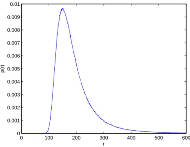
0 100 200 300 400 500 600 0 0.001 0.002 0.003 0.004 0.005 0.006 0.007 0.008 0.009 0.01 r p(r)

Figure 3.2: The probability density function of the user location distribution; r0 = 150

m.

As mentioned before, a rate balancing step is needed if the user rate constraints are not satisfied. We divide the DNs into two groups: Group I consists of DNs whose rate requirements have been met and members of Group II include all other DNs. We first select the DN, say DN i, from Group II whose rate allocation is the lowest and the one, say DN j from Group I having the largest surplus rate (Rj − Rj,min). Among the

subcarriers which have been assigned to DN j, we reassign to DN i the one which is the best for it if the reassignment does not make DN j become a member of Group II. The rate requirements for almost all DNs in Group II can be met through such a reassignment. In order not to make the process too complicated, we give up on DN i when the above reassignment is not allowed. The rate-balancing process is sequentially applied to all DNs in Group II in descending order of the allocated rate.

3.5 Numerical Results and Discussions

The simulation results shown in this section assume a single-cell network with multiple DNs that are randomly distributed within a 120-degree section of the 600-meter radius

(28)

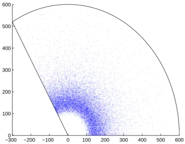
−3000 −200 −100 0 100 200 300 400 500 600 100 200 300 400 500 600

Figure 3.3: The user location distribution; r0 = 150 m.

circle centered at the BS. The RNs are placed on a circle with a 150-meter radius with a equal angular spacing. As shown in Fig. 3.2 and 3.3, the probability density function (pdf) of the DN locations is given by [20]

P = r40 r5 exp · −5 4 ³r0 r ´₄¸ . (3.11) where r > 0 is the radius and r0 = 150 m. We also assume each subcarrier suffers

from independent Rayleigh fading in any direct or relay link with a path loss exponent 3.5. For the convenience of comparison, we normalize each link gain with respect to the worst-case gain corresponding to the longest link distance.

We compare the performance of our subcarrier assignment (SA) algorithm (P2-solver) with two subcarrier assignment schemes which we refer to as greedy SA and weighted SA algorithms, respectively. These two algorithms were modified from those presented in [8] and [9], respectively. As the originally schemes were designed with perfect CSI assumption and have different RN selection criterion, we use our P1 and P3 solutions but keep that for P2 intact for the sake of fair comparison.

(29)

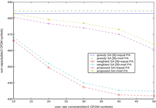
with a total system power of PT = 3.2 W (i.e. the average transmitted power for each

subcarrier is 0.1 W) and varying minimum rate requirements. The first figure shows that the sum rate of our algorithm is closer to the greedy SA than the weighted SA does. For a given subcarrier assignment scheme, we compare two power allocation methods– equal power allocation and the proposed modified water-filling power allocation for the direct link. As expected, our scheme of [4.34] performs better than the equal power allocation approach. The second figure depicts the rate failure probability behavior, i.e., the probability that the algorithm fails to meet a user’s rate requirement. Obviously, our solution has a much lower rate failure probability than those achievable by either greedy SA or weighted SA scheme. In Fig. 3.6 and Fig. 3.7 we compare the sum rate

10 15 20 25 30 35 40 45 50 430 440 450 460 470 480 490

user rate constrain(bits/2 OFDM symbols)

sum capacity(bits/2 OFDM symbols)

greedy SA [8]+equal PA greedy SA [8]+mwf PA weighted SA [9]+equal PA weighted SA [9]+mwf PA proposed SA+equal PA proposed SA+mwf PA

Figure 3.4: Sum rate v.s. user rate constraint; 8 DNs, 3 RNs and 32 subcarriers with

PT = 3.2.

and required rate failure probability (i.e., the probability that an algorithm fails to meet the rate requirement) performance as a function of the user number in a 32-subcarrier OFDMA network having 3 RNs, PT = 3.2 and a minimum user rate requirement of

(30)

10 15 20 25 30 35 40 45 50 0 0.05 0.1 0.15 0.2 0.25 0.3 0.35 0.4 0.45

required rate failure probability

greedy SA [8]+mwf PA weighted SA [9]+mwf PA proposed SA+mwf PA

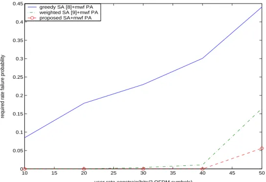
Figure 3.5: Rate failure probability v.s. user rate constraint;8 DNs, 3 RNs and 32 subcarriers with PT = 3.2.

48 bits/2 OFDM symbols. It is clear that our algorithm outperforms the weighted SA scheme. In Fig. 3.8, we examine the conditional average achievable rate ratio γ defined as γ = E [Rk/Rk,min|Rk < Rk,min], if P(Rk < Rk,min) 6= 0; otherwise γ = 1. We observe

that our algorithm is far better than the greedy algorithm and when the user number is large, outperform the weighted SA algorithm of [9]. For fair comparison, all three algorithms employ the proposed mwf power loading scheme. In Fig. 3.9, we show the average probability of doing the load balancing step. While the user number increases, users are more likely not to satisfy their rate constraints, and thus the probability of doing the load balancing step increases.

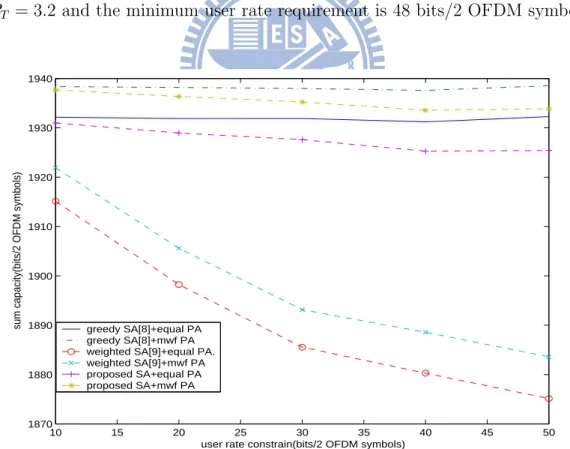
In Figs. 3.10–3.11, we consider another scenario in which there are 8 DNs, 3 RNs in a 128-subcarrier OFDMA cell with a total system power of PT = 12.8 W. They also shows

that the sum rate of our algorithm not only has the lower probability that users fail to meet their rate requirements but is closer to the greedy SA than the weighted SA does.

(31)

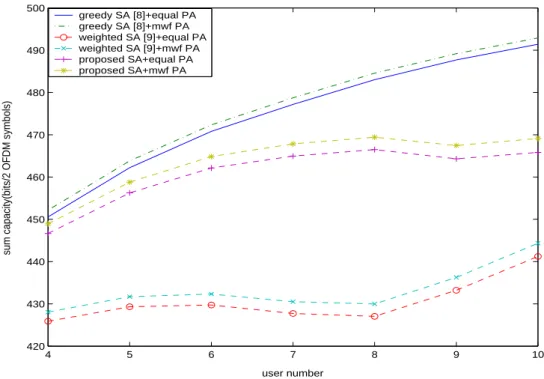
4 5 6 7 8 9 10 420 430 440 450 460 470 480 490 500 user number

greedy SA [8]+equal PA greedy SA [8]+mwf PA weighted SA [9]+equal PA weighted SA [9]+mwf PA proposed SA+equal PA proposed SA+mwf PA

Figure 3.6: Sum rate v.s. user number; 3 relay nodes and 32 subcarriers with PT = 3.2

and the minimum user rate requirement is 48 bits/2 OFDM symbols.

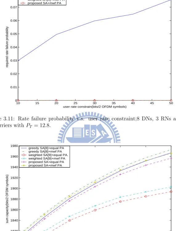
Moreover, the performance enhancement by the proposed modified water-filling power allocation for the direct link. Then in Fig. 3.12 and Fig. 3.13 we compare the sum rate and required rate failure probability performance as a function of the user number in a 128-subcarrier OFDMA network having 3 RNs, PT = 12.8 and a minimum user rate

requirement of 48 bits/2 OFDM symbols. Our algorithm also outperforms the weighted SA scheme.

(32)

4 5 6 7 8 9 10 0 0.1 0.2 0.3 0.4 0.5 0.6 0.7 user number

Figure 3.7: Rate failure probability v.s. user number; 3 relay nodes and 32 subcarriers with PT = 3.2 and the minimum user rate requirement is 48 bits/2 OFDM symbols.

4 5 6 7 8 9 10 40 50 60 70 80 90 100 user number γ

( the conditional average achievable rate ratio )(%)

Figure 3.8: Average achievable rate ratio for the rate failure event v.s. user number; 3 relay nodes and 32 subcarriers with PT = 3.2 and the minimum user rate requirement

(33)

4 5 6 7 8 9 10 0 0.1 0.2 0.3 0.4 0.5 0.6 0.7 0.8 0.9 1 user number

probability of load balancing

Figure 3.9: Load balance probability v.s. user number; 3 relay nodes and 32 subcarriers with PT = 3.2 and the minimum user rate requirement is 48 bits/2 OFDM symbols.

10 15 20 25 30 35 40 45 50 1870 1880 1890 1900 1910 1920 1930 1940

sum capacity(bits/2 OFDM symbols) greedy SA[8]+equal PA greedy SA[8]+mwf PA weighted SA[9]+equal PA. weighted SA[9]+mwf PA proposed SA+equal PA proposed SA+mwf PA

Figure 3.10: Sum rate v.s. user rate constraint; 8 DNs, 3 RNs and 128 subcarriers with

(34)

10 15 20 25 30 35 40 45 50 0 0.01 0.02 0.03 0.04 0.05 0.06 0.07 0.08

greedy SA[8]+mwf PA weighted SA[9]+mwf PA proposed SA+mwf PA

Figure 3.11: Rate failure probability v.s. user rate constraint;8 DNs, 3 RNs and 128 subcarriers with PT = 12.8. 4 5 6 7 8 9 10 1780 1800 1820 1840 1860 1880 1900 1920 1940 1960 1980 user number

greedy SA[8]+equal PA greedy SA[8]+mwf PA weighted SA[9]+equal PA. weighted SA[9]+mwf PA proposed SA+equal PA proposed SA+mwf PA

Figure 3.12: Sum rate v.s. user number; 3 relay nodes and 128 subcarriers with PT = 12.8

(35)

4 5 6 7 8 9 10 0 0.02 0.04 0.06 0.08 0.1 0.12 user number

greedy SA[8]+mwf PA weighted SA[9]+mwf PA proposed SA+mwf PA

Figure 3.13: Rate failure probability v.s. user number; 3 relay nodes and 128 subcarriers with PT = 12.8 and the minimum user rate requirement is 48 bits/2 OFDM symbols.

(36)

Chapter 4 Downlink Resource/Relay

Allocation for MIMO OFDMA

Networks

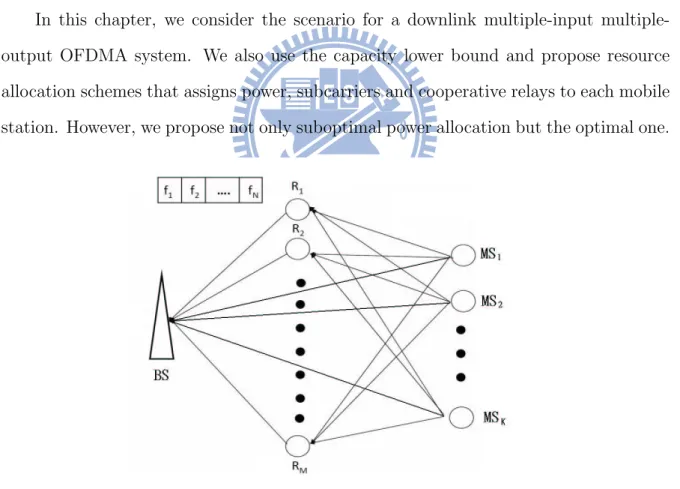
In this chapter, we consider the scenario for a downlink input multiple-output OFDMA system. We also use the capacity lower bound and propose resource allocation schemes that assigns power, subcarriers and cooperative relays to each mobile station. However, we propose not only suboptimal power allocation but the optimal one.

(37)

Figure 4.2: One cooperative path in Fig.4.1

4.1 System Model and Basic Assumptions

As shown in Fig. 4.1 and Fig. 4.2, we consider the downlink of an N-subcarrier OFDMA cooperative network which contains a BS, M fixed relay nodes, and K MS’s equipped with Ns, Nr and Nd antennas, respectively. We also consider the

decode-and-forward (DF) cooperative relay scheme and assume a two-phase (time-slot) transmission scheme with perfect timing synchronization among all network users. Perfect decoding at the relays is assumed. Each subcarrier suffers from slow flat Rayleigh fading and there is no change of the channel state during a two-phase period. A data stream from a source user must be carried by the same subcarrier no matter it is transmitted by a source node or a relay node. However, we do not employ the maximum-ratio-combining detector for this MIMO system for simplification.

We also assume the mobile user estimate the channel information by MMSE estima-tor and the feedback of the estimate is instantaneous and perfect to the BS, then the same channel information about the channel gain with an estimation error is available simultaneously to both the transmitter and the receiver. In this chapter, the BS also acts as a central control device to allocate resources based on the imperfect CSI from all users and the minimum rate requirement of each MS.

(38)

4.2 Capacity Lower Bound for MIMO Channels

First, for a source-to-destination link, we denote the estimated gain matrix of MIMO channels, estimated error matrix of MIMO channels, and noise matrix as ˆH, ˜H and W .

Than we assume the entries of ˜H and W are independent, identically distributed (i.i.d.)

and zero-mean circularly symmetric complex Gaussian (ZMCSCG) with variance σ2

h and

σ2

n, respectively.

Moreover, given the singular value decomposition(SVD) of the estimated channel matrix be ˆH = UDV∗_{, we can find that U and V are unitary matrixes and D is a}

diag-onal matrix whose diagdiag-onal entries are the singular values of ˆH. Thus, by multiplying

the transmitted signal vector by the vector V before transmitted and multiplying the received signal by the vector U∗ _{at destination, the processed received signal vector Y}

then can be expressed as

Y = U∗_{( ˆ}_{H + ˜}_{H)V X + U}∗_W _(4.1)

where X is the transmitted signal vector. And we replace ˆH by UDV∗_{, (4.1) becomes}

Y = DX + U∗_{HV X + U}˜ ∗_W _(4.2) Assume ˜H =    h11 · · · h1NS ... . .. ... hNR1 · · · uNRNS    , V =    v11 · · · v1NS ... . .. ... vNS1 · · · vNSNS    , U∗ ₌    u11 · · · u1NR ... . .. ... uNR1 · · · uNRNR    , X =    x1 ... xNS    ,

then

U∗_{H =}˜        NR P i=1 u1i˜hi1 · · · NR P i=1 u1i˜hiNS ... . .. ... NR P i=1 uNRi˜hi1 · · · NR P i=1 uNRi˜hiNS        (4.3) U∗_{HV =}_˜        NS P l=1 NR P i=1 u1i˜hilvl1 · · · NS P l=1 NR P i=1 u1i˜hilvlNS ... . .. ... NS P l=1 NR P i=1 uNRi˜hilvl1 · · · NS P l=1 NR P i=1 uNRi˜hilvlNS        (4.4)

(39)

U∗_{HV X =}_˜        NS P k=1 NS P l=1 NR P i=1 u1i˜hilvlkxk ... NS P k=1 NS P l=1 NR P i=1 uNRi˜hilvlkxk        (4.5)

Since U∗ _{is an unitary matrix, which means} NPR i=1

ut1iu∗t2i equals to 1 if t1 = t2 and

otherwise equals to zero, the entries outside the main diagonal in the covariance matrix of U∗_{HV X are zero. Moreover, for the tth diagonal entries in the covariance matrix of}˜

U∗_{HV X, we need to calculate}˜ E " ( NS X k1=1 NS X l1=1 NR X i1=1 uti1˜hi1l1vl1k1xk1)( NS X k2=1 NS X l2=1 NR X i2=1 uti2˜hi2l2vl2k2xk2)∗ # (4.6) In (4.6), we can notice that

1.Due to xk1 and xk2 are independent, E

· (PNS l1=1 NR P i1=1 uti1˜hi1l1vl1k1xk1)( NS P l2=1 NR P i2=1 uti2˜hi2l2vl2k2xk2)∗ ¸ for all k1 6= k2 are equal to zero.

2.Due to ˜hi1l1 and ˜hi2l2 are independent, E

· (PNS l1=1 NR P i1=1 uti1˜hi1l1vl1k1xk1)( NS P l2=1 NR P i2=1 uti2˜hi2l2vl2k2xk1)∗ ¸ for all l1 6= l2 or i1 6= i2 are equal to zero.

Equation (4.6) than can be rewrited as

E " ( NS X k1=1 NS X l1=1 NR X i1=1

uti1u∗ti1˜hi1l1˜h∗i1l1vl1k1vl1k1∗ xk1x∗k1)

# (4.7) which equals NR X i1=1 uti1u∗ti1 NS X l1=1 E h (˜hi1l1˜h∗i1l1) iXNS k1=1 (vl1k1vl1k1∗ )E £ xk1x∗k1 ¤ (4.8) By (4.8), since V and U∗ _{are unitary matrix, the diagonal entries of the covariance matrix}

of U∗_{HV X are all}˜ PNs k=1

kxkk2σh2. Thus, we can find that U∗HV X is still a zero-mean˜

complex gaussian vector where each entry’s variance is PNs

k=1

kxkk2σh2.

Then a tight lower bound for the capacity of the above link CLB (in bits/sec/Hz)

can be formulated as CLB = Nt X i=1 log₂(1 + _N piλi t P i=1 piσh2+ σ2n ) (4.9)

(40)

where Nt is the number of eigen-channels, pi is the power on the ith eigen-channel, and

λi is the square to ith singular value of MIMO channel. We can notice that the power

on each eigen-channel has the influence on all eigen-channels’ rates. For brevity, we will refer to link capacity and its lower bound interchangeably in the subsequence discourse unless there is danger of ambiguity.

4.2.1 Achievable Rates for RA and NRA Modes

For a decode and forward relaying scheme cooperative transmission, denote the number of antennas on source, relay, and destination as Ns, Nr, and Nd. Under DF

scheme, given min {Ns, Nr} = Nt1 and min{Nr, Nd} = Nt2, the achievable rate can be

formulated as

rm(k, n, P ) = min{

Nt1

X

i=1

log₂(1 + Pps,i_N(k, m, n)α_t1 mλs,i(k, m, n)

i=1ps,i(k, m, n)αmσ2h+ σn2

),

Nt2

X

i=1

log₂(1 + Ppr,i_N(k, m, n)α_t2 k,mλr,i(k, m, n)

i=1pr,i(k, m, n)αk,mσh2+ σn2 )} (4.10) where NPt1 i=1 ps,i= ps, Nt2 P i=1

pr,i = pr, ps+ pr = P and λs,i and λr,i are denoted the square to

the ith singular values of the source-relay and relay-destination MIMO channels sorted in descending order and αs and αr are the path losses of the source-relay and

relay-destination paths.

Moreover, for the NRA mode, we allow the source to be active for both phases, a fair comparison on the achievable rate should be measured with respect to the total consumed energy. The resulting link capacity over two OFDM symbols is

rD(k, n, P ) = 2 Nt X i=1 log₂(1 + pi(k,n) 2 αkλs,i(k, n) Nt P i=1 pi(k,n) 2 αkσh2+ σ2n ) (4.11) where pi(k, n) is the power on the ith eigen-channel, Nt = min {Ns, Nd} and αk is the

(41)

4.3 Problem Statement

We also use the subcarrier assignment and link selection indicator ρ(k,n,m)mentioned

before. When ρ(k,n,m) = 1 and m > 0, it indicates subcarrier n is allocated to user k

who options for RA mode using relay node m while m = 0 it indicates the user options for the NRA mode. Otherwise, user k does not have access to subcarrier n over the mth link. We also suppose the available total transmission power is PT, then the problem of

maximizing the total system rate under the users’ rate constraints is equivalent to

max K X k=1 Rk= max K X k=1 N X n=1 M X m=0 ρ(n,k,m)rm(k, n, P (k, m, n)) subject to Rk≥ Rk,min ∀k K X k=1 M X m=0 ρ(k,n,m)≤ 1 ∀n ρ(k,n,m) ∈ {0, 1} ∀ n, k, m N X n=1 K X k=1 M X m=0 ρ(k,n,m)P (k, m, n) ≤ PT (4.12) P (k, m, n) ≥ 0 ∀ n, k, m, i

where Rkand Rk,min are the achievable rate and the minimum rate requirement for user

k, and r0(k, n, P ) = rD(k, n, P ).

In next section, we propose a low-complexity suboptimal algorithm due to the above formulation is also an NP-hard mixed integer programming problem which is hard to find the optimal solution.

4.4 Resource Allocation Schemes in MIMO

Chan-nels

For the optimization problem in MIMO system, we also decompose resource al-location schemes into a three subproblems as mentioned in Chap.3: P1–link selection

(42)

subproblem for deciding {βm(n, k)}, P2–subcarrier assignment for deciding {δ(n,k)}, and

P3–power allocation.

4.4.1 Relaying/Direct Link Selection Rule and Subcarrier

As-signment

Since in the relaying/direct link selection step, the final power allocation is still unknown, we then assume a fair power distribution P = PT

N for all DNs. Under such

assumption, for a relay-assisted subcarrier n for user k relayed by relay m, we need to find not only the optimal power ratio of relay to source such that the power is efficiently used but the optimal power allocation on each eigen-channel, thus the problem can be formulated as max rm(k, n, P ) subject to rm(k, n, P ) ≤ Nt1 X i=1

log₂(1 + Pps,i_N(k, m, n)α_t1 mλs,i(k, m, n)

i=1ps,i(k, m, n)αmσh2+ σn2 ) rm(k, n, P ) ≤ Nt2 X i=1

log₂(1 + Ppr,i_N(k, m, n)α_t2 k,mλr,i(k, m, n)

i=1pr,i(k, m, n)αk,mσh2+ σn2 ) Nt1 X i=1 ps,i(k, m, n) + Nt2 X i=1 pr,i(k, m, n) ≤ PT N ps,i(k, m, n)) ≥ 0, pr,i(k, m, n)) ≥ 0, ∀ i, k, m By assuming Ps(k, m, n) = P_N_t1

i=1ps,i(k, m, n) and Pr(k, m, n) =

P_N_t2

i=1pr,i(k, m, n), we

(43)

Subproblem 1: max rm(k, n, P ) subject to rm(k, n, P ) ≤ Nt1 X i=1

log₂(1 + ps,i(k, m, n)αmλs,i(k, m, n)

Ps(k, m, n)αmσ_h2+ σn2 ) rm(k, n, P ) ≤ Nt2 X i=1

log₂(1 + pr,i(k, m, n)αk,mλr,i(k, m, n)

Pr(k, m, n)αk,mσ_h2+ σn2 ) Ps(k, m, n) + Pr(k, m, n) ≤ PT N ps,i(k, m, n)) ≥ 0, pr,i(k, m, n)) ≥ 0, ∀ i, k, m Subproblem 2: For SR path: max Nt1 X i=1

Ps(k, m, n)αmσh2+ σ2n ) subject to Nt1 X i=1 ps,i(k, m, n) ≤ Ps(k, m, n) (4.13) ps,i(k, m, n)) ≥ 0 ∀ i, k, m For RD path: max Nt2 X i=1

Pr(k, m, n)αk,mσh2 + σn2 ) subject to Nt2 X i=1 pr,i(k, m, n) ≤ Pr(k, m, n) (4.14) pr,i(k, m, n)) ≥ 0 ∀ i, k, m

For each subproblem 2, we can derive the optimal power allocated on subcarrier n’s SR and RD eigen-channels from the water-filling solution

ps,i(k, m, n) = µ µs,n− αmPs(k, m, n)σ2h+ σn2 αmλs,i(k, m, n) ¶₊ (4.15)

(44)

pr,i(k, m, n) = µ µr,n− αm,kPr(k, m, n)σ2h+ σn2 αm,kλr,i(k, m, n) ¶₊ (4.16) where µs,n and µr,n are inner water-levels which mean the water-levels controlling the

power of eigen-channels.

We now assume the number of the eigen-channels of subcarrier n on SR and RD path allocated positive power are κs(n) and κr(n), respectively, then from (4.15) and (4.16),

the inner water-level µs,n and µr,n that satisfies the subcarrier power constraint (4.13)

and (4.14) can be expressed as

µs,n = 1 κs(n)  Ps(k, m, n) + αmPs(k, m, n)σh2 + σn αm κ_Xs(n) i=1 1 λs,i(k, m, n)   _(4.17) µr,n = 1 κr(n)  Pr(k, m, n) + αm,kPr(k, m, n)σh2+ σn αm,k κ_Xr(n) i=1 1 λr,i(k, m, n)   _(4.18) Thus, the rate of subcarrier n on SR/RD link can be formulated as

Rs(k, m, n) = Nt1 X i=1 rs,i(k, m, n) = κ_Xs(n) i=1

log₂(1 + αmps,i(k, m, n)λs,i(k, m, n)

αmPs(k, m, n)σh2 + σn2 ) = κ_Xs(n) i=1 log₂( αmµs,nλs,i(k, m, n) αmPs(k, m, n)σ2h+ σn2 ) (4.19) Rr(k, m, n) = Nt2 X i=1 rr,i(k, m, n) = κ_Xr(n) i=1

log₂(1 + αk,mpr,i(k, m, n)λr,i(k, m, n)

αk,mPr(k, m, n)σ2h+ σn2 ) = κ_Xr(n) i=1 log₂( αk,mµr,nλr,i(k, m, n) αk,mPr(k, m, n)σ2h+ σn2 ) (4.20)

(45)

Moreover, the lagrange function of subproblem 1 is L = rm(k, n, P ) + λn,s( Nt1 X i=1

Ps(k, m, n)αmσh2+ σ2n ) − rm(k, n, P ))) + λn,r( Nt2 X i=1

Pr(k, m, n)αk,mσh2+ σ2n

) − rm(k, n, P ))

+ λP(

PT

N − Ps(k, m, n) − Pr(k, m, n)) (4.21)

where λn,s, λn,r and λP are lagrange multipliers. Based on (4.17) and (4.19), we

differ-entiate the lagrange function (4.21) by Ps(k, m, n) and let the resulting function equal

to 0, then the optimal solution of Ps(k, m, n) in subproblem1 can be obtained by the

quadratic formula Ps(k, m, n) = −b +√b2_{− 4ac} 2a (4.22) where a = αmσh2 σ2 n Ã 1 + σ2 h κPs(n) i=1 1 λs,i(k,m,n) ! , b = 1 + 2σ2 h κPs(n) i=1 1 λs,i(k,m,n), c = − Ã λn,sκs(n) λpln 2 − σ2 n αm κPs(n) i=1 1 λs,i(k,n) !₊

Also, based on (4.18) and (4.20), we can derive Pr(k, m, n) by differentiating the lagrange

function (4.21) by Pr(k, m, n) Pr(k, m, n) = −b +√b2_{− 4ac} 2a (4.23) where a = αk,mσ2h σ2 n Ã 1 + σ2 h κPr(n) i=1 1 λr,i(k,m,n) ! , b = 1 + 2σ2 h κPr(n) i=1 1 λr,i(k,m,n), c = − Ã λn,rκr(n) λpln 2 − σ2 n α_k,m κPr(n) i=1 1 λr,i(k,n) !₊

(46)

la-grange function (4.21) by rm(k, n):

λn,s+ λn,r = 1 (4.24)

The final step is to adjust all lagrange multipliers until the power constraint in subprob-lem 1 is satisfied and Rs(k, m, n) = Rr(k, m, n) for having the best power efficiency. The

maximum rm(k, n,P_NT) is denoted by r∗m(k, n,PNT). Notice that the ratio of Pr(k, m, n)

to Ps(k, m, n) is the optimal ratio when given P = P_NT.

Moreover, considering about the direct link, the power allocation problem can be formulated as max rD(k, n, PT N ) subject to Nt X i=1 pi(k, n) = PT N (4.25) pi(k, n) ≥ 0 ∀ i, k

we can derive the optimal power allocated on each of its eigen-channel is

pi(k, n) = µ µn− αk 2 P (k, n)σ2h+ σn2 αk 2 λs,i(k, n) ¶+ (4.26) By tuning the water-level µn to satisfy the total power constraint, we can find the

maximum rD(k, n,P_NT) and denote it by r0∗(k, n,PNT).

We then determine the relay who can achieve the highest rate for user k on subcarrier

n, whcih can be formulated as

m∗ _{= arg max} 0≤m≤Mr ∗ m(k, n, PT N ) (4.27)

When m∗ _{= 0, DN k should use only the direct link if it was given subcarrier n. We}

then set βm∗(n, k) = 1 and β_m(n, k) = 0, for 0 ≤ m ≤ M, m 6= m∗.

However, for the subcarrier assignment in MIMO systems, we also use the subcarrier assignment algorithm summarized in Table (3.1).

(47)

4.4.2 Power Allocation

After the relaying/direct link selection and subcarrier assignment, we now suggest a nearly optimal power allocation scheme and the optimal power allocation scheme. I Nearly Optimal Power Allocation

Similar to the SISO case, we first assign equal power PT/N to subcarriers using

relaying and then allocate the remaining power by a modified water-filling (mwf) on subcarriers using no relays. Thus, for NRA subcarriers, our power allocation problem can be formulated as max K X k=1 X n∈U0 ρ(n,k,0)r0(k, n, p1(k, 0, n), · · · , pNt(k, 0, n)) subject to K X k=1 X n∈U0 ρ(k,n,0) Nt X i=1 pi(k, 0, n) ≤ PN RA (4.28) pi(k, 0, n) ≥ 0 ∀ n, k, i

where U0 is the set of NRA subcarriers and PN RA is the remaining power for NRA

subcarriers. However, by assuming PNt

i=1pi(k, 0, n) = P (k, n), we can decompose this

problem into two subproblems: Subproblem 1: max K X k=1 X n∈U0 ρ(n,k,0)r0(k, n, P (k, n)) subject to K X k=1 X n∈U0 ρ(k,n,0)P (k, n) ≤ PN RA (4.29) P (k, n) ≥ 0 ∀ n

(48)

Subproblem 2: for each subcarrier n in U0 max K X k=1 ρ(n,k,0)r0(k, n, p1(k, 0, n), · · · , pNt(k, 0, n)) subject to K X k=1 ρ(k,n,0) Nt X i=1 pi(k, 0, n) = P (k, n) (4.30) pi(k, 0, n) ≥ 0 ∀ i, k

For the subproblem 2 of each subcarrier n in U0, we can derive the optimal power

allocation on each of its eigen-channel

pi(k, 0, n) = µ µn− αk 2 P (k, n)σh2+ σ2n αk 2 λs,i(k, n) ¶+ (4.31) where µn is the water level. Assume the number of the eigen-channel of subcarrier n

allocated positive power is κ(n), then from (4.31), the water-level µn that satisfies the

subcarrier power constraint (4.30) can be expressed as

µn= 1 κ(n)  P (k, n) + α2kP (k, n)σh2+ σn αk 2 κ(n) X i=1 1 λs,i(k, n)   _(4.32) Thus, the rate of subcarrier n is

RD(k, n, P (k, n)) = Nt X i=1 ri(k, n) = κ(n) X i=1 2 log₂(1 + αk 2 pi(k, 0, n)λs,i(k, n) αk 2 P (k, n)σh2+ σn2 ) = κ(n) X i=1 2 log₂( αk 2 µnλs,i(k, n) αk 2 P (k, n)σh2+ σn2 ) (4.33) Based on (4.32) and (4.33), the optimal solution of subproblem1 can be obtained by the quadratic formula P (k, n) = −b + √ b2_{− 4ac} 2a (4.34) where a = αkσh2 2σ2 n Ã 1 + σ2 h κ(n)_P i=1 1 λs,i(k,n) ! ,

(49)

b = 1 + 2σ2 h κ(n)_P i=1 1 λs,i(k,n), c = − Ã 2κ(n) λ ln 2 − 2σ2 n α_k κ(n)_P i=1 1 λs,i(k,n) !₊

and (t)+ _{=max(0, t). By iteratively modifying λ to satisfy the total power constraint}

(4.29), we obtain the optimal power allocation for subcarriers using only direct link. So, the proposed power allocation for NRA subcarriers can be summarized as :

Given PN RA, ρ(n,k,0), P (k, n) = 0 and pi(k, n) = 0 for all k, n, i

Set U0 = ½ n|PK k=1 ρn,k,0 = 1 ¾ , κ(n) = Nt for n ∈ U0 while ( ¯ ¯ ¯ ¯ K P k=1 P n∈U0 P (k, n) − PN RA ¯ ¯ ¯ ¯ ≥ ²)

modify λ and calculate P (k, n) by (4.34) for user k such that ρ(n,k,0)= 1

for (n = 1 to |U0|)

calculate µn by (4.32) and pi(k, n) by (4.31)

Un= { i | pi(n, k) > 0}

while (|Un| 6= κ(n))

modify to the correct κ(n) end

end end

I Optimal Power Allocation

For the optimal power allocation, the optimization problem can be formulated as max K X k=1 Rk= max K X k=1 N X n=1 M X m=0 ρ(n,k,m)rm(k, n, P (k, m, n)) subject to N X n=1 K X k=1 M X m=0 ρ(k,n,m)P (k, m, n) ≤ PT (4.35) P (k, m, n) ≥ 0 ∀ n, k, m

The power allocated on the NRA subcarriers has been shown in nearly optimal power allocation, so we first introduce the power allocation on the RA subcarriers.

For RA subcarriers, by assumingPNt1

i=1ps,i(k, m, n) = Ps(k, m, n) and

P_N_t2

i=1pr,i(k, m, n) =

(50)

decom-pose the optimization problem into two subproblems: Subproblem 1: max K X k=1 X n∈U1 M X m=1 ρ(n,k,m)rm(k, n) subject to rm(k, n) ≤ Nt1 X i=1

Ps(k, m, n)αmσ2h+ σn2 ) ∀ n, k, m rm(k, n) ≤ Nt2 X i=1

Pr(k, m, n)αk,mσ2h+ σn2 ) ∀ n, k, m K X k=1 X n∈U1 M X m=1 ρ(k,n,m)(Ps(k, m, n) + Pr(k, m, n)) ≤ PRA (4.36) Ps(k, m, n) ≥ 0, Pr(k, m, n) ≥ 0 ∀ n, k, m

where U1 is the set of NRA subcarriers and PRA is the total power of NRA subcarriers.

The first and second constraints are due to the rate of the cooperative transmission is the minimum of the rate of SR and of RD link.

Subproblem 2: for each RA subcarrier n in U1

For SR path: max K X k=1 M X m=1 ρ(k,n,m) Nt1 X i=1

log₂(1 + ps,iαmλs,i(k, m, n)

Psαmσh2+ σ2n ) subject to K X k=1 M X m=1 ρ(k,n,m) Nt1 X i=1 ps,i(k, m, n) = Ps(k, m, n) (4.37) ps,i(k, m, n)) ≥ 0, ∀ i, k, m For RD path: max K X k=1 M X m=1 ρ(k,n,m) Nt2 X i=1

log₂(1 + pr,iαk,mλr,i(k, m, n)

Prαk,mσh2+ σn2 ) subject to K X k=1 M X m=1 ρ(k,n,m) Nt2 X i=1 pr,i(k, m, n) = Pr(k, m, n) (4.38) pr,i(k, m, n) ≥ 0 ∀ i, k, m

(51)

For each subproblem 2, we have derived the optimal power allocated on subcarrier n’s SR and RD eigen-channels from the water-filling solution in (4.15) and (4.16). We now also assume the number of the eigen-channels of subcarrier n on SR and RD path allocated positive power are κs(n) and κr(n), respectively. Moreover, the lagrange function of

subproblem 1 can be expressed as

L = K X k=1 X n∈U1 M X m=1 ρ(n,k,m){rm(k, n) + λn,s(k, m, n)( Nt1 X i=1

Ps(k, m, n)αmσ2h+ σn2 ) − rm(k, n)) + λn,r(k, m, n)( Nt2 X i=1

Pr(k, m, n)αk,mσh2+ σ2n ) − rm(k, n))} + λP(PRA− K X k=1 X n∈U1 M X m=1 ρ(k,n,m)(Ps(k, m, n) + Pr(k, m, n))) (4.39)

where λn,s(k, m, n), λn,r(k, m, n) and λP are lagrange multipliers.

Based on (4.17) and (4.19), we differentiate the lagrange function (4.39) by Ps(k, m, n)

and let the resulting function equal to zero, then the optimal solution of Ps(k, m, n) in

subproblem1 is the same as (4.22). By the same way, the optimal Pr(k, m, n) is as

ex-pressed in (4.23). Moreover, by differentiating the lagrange function (4.39) by rm(k, n),

the relationship between λn,s(k, m, n) and λn,r(k, m, n) is also the equation we showed

in (4.24). We then need to adjust all lagrange multipliers until all power constraints are satisfied and Rs(k, m, n) = Rr(k, m, n) for all k, m, n. Finally, the resulting proposed

optimal power allocation is summarized in Table 4.1.

4.5 Numerical Results and Discussions

The simulation results shown in this section assume a single-cell network with multiple DNs that are uniformly distributed within a 120-degree section of the 600-meter radius circle centered at the BS. The RNs are placed on a circle with a 150-meter radius with a equal angular spacing. We also assume each subcarrier suffers from independent Rayleigh

正交分頻多工存取下載系統在非完全通道資訊下之資源分配及中繼器選取

國 立 交 通 大 學

電信工程研究所

碩 士 論 文

正交分頻多工存取下載系統在非完全通道資訊下之

資源分配及中繼器選取

Downlink Resource Allocation and Relay Selection

for OFDMA Networks With Imperfect Channel

Information

研究生：王俊鋐

指導教授：蘇育德 博士

正交分頻多工存取下載系統在

非完全通道資訊下之資源分配及中繼器選取

Downlink Resource Allocation and Relay Selection

for OFDMA Networks With Imperfect Channel Information

研究生：王俊鋐 Student：Jiun-Hung Wang

指導教授：蘇育德博士 Advisor：Dr. Yu T. Su

國 立 交 通 大 學

電 信 工 程 研 究 所

碩 士 論 文

正交分頻多工存取下載系統在非完全通道

資訊下之資源分配及中繼器選取

研究生：王俊鋐 指導教授：蘇育德 博士

國立交通大學電信工程研究所碩士班

中文摘要

正交分頻多工存取(OFDMA)系統可以利用簡單的通道等化器來有效

的避免頻率選擇性衰減並使用最小（Nyquist）次載波距（subcarrier spacing）

來提高頻譜效能。這種多工技術也容許很有彈性的資源分配，以充分利用

不同用戶的通道狀況，一則可滿足個別用戶傳送速率的要求，另則可最大

化整個系統的通道容量。此外，由於電磁信號傳播的統計特性，蜂巢式行

動通訊系統之收訊強度無法定量保證，其中難免有部分用戶收訊品質不

佳。一個經濟有效的解決方案便是中繼站的設立，適當的佈建中繼站不但

有助於提升其信號品質，並可擴增基地台的覆蓋範圍與容量。

本論文主要在研究有多座中繼站的 OFDMA 下鏈系統之資源分配及中

繼站選取的問題。我們同時考慮傳送（基地台）與接收（用戶）端皆使用

單一天線(SISO)以及兩端皆有多根天線(MIMO)兩種架構，而下傳時雖有多

個中繼站可以挑選，但各通道狀況的資訊卻有不確定性；亦即，基地台只

有通道狀況的估計值以及誤差機率分佈。我們使用在此不確定情況下的通

道容量下限來作為系統效能的評估標準。對上述 SISO 與 MIMO 兩種架構

下，我們都推導出傳送端與中繼站的最佳功率比來達到最大的通道容量下

ii

限。根據這個功率比我們分別提出了幾近最佳的次載波及其能量（功率）

分配的演算法。我們的演算法複雜度不高，電腦模擬結果也顯示它能兼顧

個別用戶的公平性，滿足其傳送速率要求也可以令系統的整體傳送速率達

到最大值。

Downlink Resource Allocation and Relay Selection

for OFDMA Networks With Imperfect Channel

Information

誌 謝

對於論文得以順利完成，首先感謝我的指導教授 蘇育德博士。老師

除了在專業上面的教導之外，做人處世的態度也令我受益匪淺。另外也感

謝口試委員蘇賜麟教授、林茂昭教授、呂忠津教授以及吳卓諭教授給予的

寶貴意見，以補足這分論文的缺失與不足之處。而在實驗室方面，也特別

感謝林淵斌學長、劉人仰學長、張致遠學長、劉彥成學長以及其他學長姐、

同學和學弟妹在這兩年內的不論是研究上或上生活上的幫忙與鼓勵。

最後，感謝一路上不斷支持我的家人，他們的關心與鼓勵帶給了我無

形的動力，僅獻上此論文，以代表我最深的敬意。

Contents

List of Figures

List of Tables

Chapter 1

Introduction

Chapter 2

Relay System and Cooperative

Transmission

2.1

Relay Networks

2.2

Relay Strategies

2.3

Capacity of Cooperative Transmissions

Chapter 3

Downlink Resource/Relay

Allocation for SISO OFDMA

Networks

3.1

System Model and Assumptions

3.2

Achievable rates for RA and NRA modes

3.3

國立交通大學

碩士論文

指導教授：蘇育德博士

國立交通大學

電信工程研究所

碩士論文

研究生：王俊鋐指導教授：蘇育德博士

誌謝

對於論文得以順利完成，首先感謝我的指導教授蘇育德博士。老師