移動WiMAX系統之導引碼輔助疊代式通道估測

(1)

國

立

交

通

大

學

電子工程學系電子研究所碩士班

碩

士

論

文

移動 WiMAX 系統之導引碼輔助

疊代式通道估測

Pilot-Assisted Iterative Channel Estimation for

Mobile WiMAX Systems

研究生：陳錫祺

指導教授：簡鳳村博士

(2)

(3)

移動 WiMAX 系統之導引碼輔助疊代式通道估測

Pilot-Assisted Iterative Channel Estimation for Mobile

WiMAX Systems

研究生: 陳錫祺

Student: Shi-Chi Chen

指導教授: 簡鳳村

Advisor: Dr. Feng-Tsun Chien

國立交通大學

電子工程學系電子研究所碩士班

碩士論文

A Thesis

Submitted to Department of Electronics Engineering & Institute of Electronics College of Electrical and Computer Engineering

National Chiao Tung University in Partial Fulfillment of the Requirements

for the Degree of Master in

Electronics Engineering

June 2007

HsinChu, Taiwan, Republic of China

(4)

(5)

移動 WiMAX 系統之導引碼輔助

疊代式通道估測

研究生: 陳錫祺

指導教授: 簡鳳村博士

國立交通大學

電子工程學系電子研究所碩士班

摘要

正交分頻多工系統為新一代無線通訊系統最常使用的技術，如IEEE 802.11 a/g/n， IEEE

802.16， IEEE 802.20，數位電視，數位廣播等許多系統均採用此技術。移動傳輸是未來無線通訊系統的趨勢之一，如IEEE 802.16-2005 可支援到車速 120 km/hr，而 IEEE 802.20 更可以支援到車速 250 km/hr。許多通道估測法，使用大量的導引符號，以及緩衝暫存器來估測通道。在本論文中，我們使用兩種通道估測，decision directed 和 expectation maximization。此通道估測可追蹤時變通道,以及使用少量導引符號。最後，藉由電腦模擬驗證此一新演算法在移動的環境中並使用 IEEE 802.16-2005 的規格下，可有效的改善錯誤率。

(6)

(7)

Pilot-Assisted Iterative Channel Estimation

for Mobile WiMAX Systems

Student: Shi-Chi Chen

Advisor: Dr. Feng-Tsun Chien

Department of Electronic Engineering &

Institute of Electronics

National Chiao Tung University

Abstract

Orthogonal Frequency Division Multiplexing (OFDM) is a popular technique in modern wireless communications. There are many systems adopting the OFDM technique, such as IEEE 802.11 a/g/n, IEEE 802.16, IEEE 802.20, and Digital Video Broadcasting, etc. On the other hand, mobility is an important issue that needs to be taken into account in the design of future wireless communication systems. For example, IEEE 802.16-2005 supports vehicle speed up to 120 km/hr, and IEEE 802.20 supports vehicle speed up to 250 km/hr, causing the channel seen by the receiver time-varying. Some channel estimators use a large number of pilot symbols to estimate the channel parameters, or use buffer to obtain desired channel parameters. In this thesis, we show two channel estimation approaches, namely the decision directed based and expectation maximization based approaches that can track the time-varying channel vectors with less insertion of pilot symbols. Finally, we evaluate the performance of the proposed systems under mobility using IEEE 802.16-2005 standard and confirm that it achieves good SER performance.

(8)

(9)

誌謝

這篇論文能夠順利完成，最重要感謝的人是我的指導教授簡鳳村老師。在這二年的研究生涯中，老師不僅在做研究上給予指導，讓我在知識的探索上獲益良多，同時也關心我們的日常生活。另外，要感謝的是與我在通訊領域之中一起討論、研究的洪崑健與林鴻志學長，謝謝你們熱心地幫我解決了許多通訊方面相關的疑問。也感謝從大學到研究所都一直共同打拼的耀鈞、柏昇、政達、介遠、志岡、凱庭、依翎，在修課中遇到問題時，大家互相討論，解決難題，讓我在這之中成長許多。也感謝實驗室的其他成員，在碩士這兩年中帶給我歡樂、成長，在生活上給我支持、勉勵，使我充滿信心。也感謝通訊電子與訊號處理實驗室(commlab)，提供了充足的軟硬體資源，讓我在研究中不虞匱乏。在此僅以這篇論文獻給所有幫助過我，陪伴我走過這一段歲月的師長，同學，朋友與家人，謝謝! 誌於 2007.7 風城交大錫祺

(10)

(11)

List of Figures

Fig. 2-1 Cyclic prefix is a copy of the last part of the OFDM symbol. ... 8

Fig. 2-2 A symbolic picture of the individual subchannels for an OFDM system with N tones over a bandwidth W ... 11

Fig. 2-3 Baseband OFDM system model... 12

Fig. 2-4 Continuous-time OFDM system interpreted as parallel Gaussian channels. ... 16

Fig. 2-5 Discrete-time OFDM system... 16

Fig. 2-6 Comparison of subcarrier allocatins in OFDM and OFDMA (from [8])... 19

Fig. 2-7 Subcarrier allocation in an OFDMA symbol (from [9]). ... 20

Fig. 2-8 OFDMA frequency description (3-channel schematic example, from [4]). ... 23

Fig. 2-9 Example of the data region which defines the OFDMA allocation (from [4]). ... 24

Fig. 2-10 Example of an OFDMA frame (with only mandatory zone) in TDD mode (from [2]). ... 27

Fig. 2-11 Illustration of OFDMA with multiple zones (from [2])... 28

Fig. 2-12 FCH subchannel allocation for all 3 segments (from [4])... 29

Fig. 2-13 Example of DL renumbering the allocated subchannels for segment 1 in PUSC(from [4]). ... 30

Fig. 2-14 DL cluster structure (from[10]). ... 32

Fig. 3-1 Channel estimation structure ... 43

Fig. 3-2 Pilot Symbol Aided ... 45

Fig. 3-3 Initial channel H_Np... 45

Fig. 3-4 Low pass filter... 47

Fig. 3-5 Real channel impulse response ... 47

Fig. 3-6 Real channel frequency response ... 47

Fig. 3-7 Initial channel impulse responseh_Np... 48

Fig. 3-8 Initial channel frequency responseH_Np ... 48

Fig. 3-9 Initial channel impulse responseh_Np... 49

Fig. 3-10 Initial channel frequency responseH_Np ... 49

Fig. 3-11 Final resource of the channel impulse response. ... 50

Fig. 3-12 Linear Prediction ... 51

Fig. 3-13 Linear Interpolation ... 53

Fig. 3-14 Decision directed iteration process... 55

(14)

Fig. 3-16 SER performance for DD in 100 km/hr ... 64

Fig. 4-1 EM Algorithm iteration process ... 70

Fig. 4-2 SER performance for EM in 240 km/hr ... 78

(15)

List of Tables

Table 2-1 OFDM Advantages and Disadvantages ... 19

Table 2-2 S–OFDMA Parameters Proposed by WiMAX Forum... 26

Table 2-3 1024-FFT OFDMA DL Carrier Allocation for PUSC ... 33

Table 3-1 System Parameters Used in Our Study ... 56

Table 3-2 Terrain Type vs. SUI Channels ... 57

Table 3-3 General characteristics of SUI channels ... 58

Table 3-4 SUI-1 Channel Model ... 59

Table 3-10 ETSI “Vehicular A” Channel Model in Different Units ... 61

(16)

Chapter 1 Introduction

1.1 Significance

Wireless communication systems have been in use for quite a long time. Many standards are available based on which user devices communicate, but the present standards fail to provide sufficient data rate, when the user is moving at high speed. Broadband wireless access is an appealing way to provide flexible and easily-to-deploy solution for high speed communications. In view of this requirement for future mobile wireless communication systems, the 802.16 standard has been proposed by Institute of Electrical and Electronic Engineers (IEEE) [1][3]

The WiMAX (Worldwide Interoperability for Microwave Access) Forum is committed to providing optimized solutions for fixed, nomadic, portable and mobile broad band wireless access. Two versions of WiMAX address the demand for different type of access:

z IEEE 802.16-2004: This is based on the 802.16-2004 version of the IEEE 802.16 standard. It uses Orthogonal Frequency Division Multiplexing (OFDM) and supports fixed and nomadic access in Line of Sight (LOS) and Non Line of Sight (NLOS) environments. For LOS environment, the frequency range in 802.16d is from 2GHz to 66GHz and Single Carrier (SC) is mainly adopted as the

(17)

transmission scheme. For NLOS environment, it focuses on the Broadband Wireless Access (BWA), where the frequency band ranges from 2GHz to 10GHz. In

physical layer (PHY), NLOS temps to adopt OFDM and OFDMA techniques. z IEEE 802.16-2005: optimized for dynamic mobile radio channels. This version is

based on the IEEE 802.16-2005 amendment and provides support for handoffs and roaming. The choice of the subcarrier number becomes more flexible since it provides four options, 128, 512, 1024, 2048, in contrast to the single choice of 2048 in IEEE 802.16-2004. the frequency band ranges from 2GHz to 6GHz.

Orthogonal Frequency Division Multiplexing (OFDM) is a popular technique in modern wireless communication systems. In an OFDM system, the bandwidth is divided into several orthogonal subchannels for transmission. A cyclic prefix (CP) is inserted before each symbol. Therefore, if the delay spread of the channel is shorter than the length of the cyclic prefix, the intercarrier symbol interference (ISI) can be eliminated due to the cyclic prefix. On the other hand, subcarriers in OFDM system are orthogonal to each other over time-invariant channels, so the conventional OFDM system only requires one-tap equalizers [5] to compensate the channel response. This characteristic simplifies the design of the OFDM receiver, and for this reason, the OFDM technique is widely used in wireless communication systems.

1.2 Motivation

Mobile transmission is a trend in future wireless communications. Many systems support the mobile transmission. While the OFDM system is applied in mobile environments, the

(18)

reliability of OFDM is limited because of the time-varying nature of the channel. A simple solution of the channel estimation is Pilot-Symbol-Aided. This solution makes each symbol has its own pilot. For these pilots, we can estimate these channels respective. Obviously, this way decreases data rate of transmission. We want to reduce pilot number of OFDM system.

We assumed that the power spectral density of channel environment is modeled using Jakes’ U-shaped function corresponding to the uniform angular distribution of the received energy at the receiver antenna [27]. In the case, the covariance function of the channel process is given by

( )

{

}

2

(

)

0 , h k k m h d C m =E h h∗ ₋ =

σ

J Ω m Where 2

( )

₀ h Ch

σ = , 2Ω =_d πF T_d _s, F is the Doppler spread of the fading channel, _d T is _s the sample time, m is the sample index, and J₀

( )

⋅ denotes the Bessel function of the first

kind and zero order.

Base on this assumption, we know that the channel environment has some correlation at different times. Some channel estimators have been proposed in earlier work [[18, [24, [25, [26]. One simple method is Pilot-Symbol-Aided Channel Estimation [18][24][25]. In a Pilot-Symbol-Aided system, pilot symbols from a known pseudorandom-symbol sequence are multiplexed with data symbols for transmission. The receiver has a prior knowledge of the pilot symbol sequence and channel estimation can be facilitated with the assistance of these

(19)

known pilot symbols. The received signal can subsequently estimate and compensate for the fading effects on the data symbols. In this method, the number of pilot symbol is large. The data rate of the OFDM system is therefore not in good condition. Some other channel estimators are implemented to increase the data rate of the transmission. One direct method is Linear Interpolation channel estimation [25][26]. This scheme inserts known pilot symbols periodically both in the time and frequency dimension to track the time variation and frequency selectivity of the channel. At the receiver, the channel complex gain at the pilot symbol positions can be easily obtained from the received signal and the known pilot symbols. Interpolation is then applied to derive the estimate of the channel knowledge at data symbol positions. Pilot patterns and interpolation methods have been extensively studied in the literature. Besides linear interpolation, linear prediction is also considered as a viable approach to perform the channel estimation [15].

An important part of a receiver design is to develop accurate models for the channel as well as advanced estimation methods to estimate the model parameters. However, the system performance can also be improved by a more optimal signal design. In [15], by modeling the multipath fading channel with a complex bandpass autoregressive (AR) model, the structure of the transmitted signal is made to vary as a function of time and/or frequency according to the prevailing channel conditions. Therefore, the accurate channel modeling and advanced estimation methods are of great importance from the adaptive transmitter point of view also.

The initial channel can be obtained by these three methods, Pilot-Symbol-Aided, Linear Interpolation, and Linear Prediction. The initial channel estimate may be a sketchy channel. If

(20)

we want to obtain a more accurate channel gains, some iteration approaches can be applied. One is Low Pass Filter Fig. 3-4, the other is Expectation Maximization (EM) algorithm [16]. The EM algorithm is a technique for finding the maximum likelihood (ML) estimates of system parameters in a broad range of problems where observed data are incomplete. The EM algorithm consists of two iterative steps: the expectation (E) step and the maximization (M) step. The E-step is performed with respect to the unknown underlying parameters, using current estimates of the parameters, conditioned upon the incomplete observations. The M-step then provides new estimates of the parameters that maximize the expectation of the log-likelihood function defined over complete data, conditioned on the most recent observation and the last estimate. These two steps are iterated until the estimated values converge. The details are discussed in Chapter 3 and Chapter 4.

1.3 Contribution

In this thesis, several channel estimation techniques are discussed. We combine and apply them to the Orthogonal Frequency Division Multiplexing (OFDM) system. In Chapter 3, the channel environments and Decision directed Channel Estimation are introduced. We choose SUI-3, SUI-3 and Vehicular A to run the computer simulations. In Chapter 4, the Expectation Maximization algorithm based Channel Estimation is considered.

Finally, we compare and analyse the SER performance of the proposed estimators. For the result, the EM-AR can work on time and does not use any buffer to save data. The EM-Linear Interpolation can work as well as EM-AR, but it has to use some buffer, which is

(21)

not desirable in real-time applications. No mater in high speed or low speed, the Expectation Maximization Channel Estimation can work very well.

(22)

Chapter 2 Overview of WiMAX System

2.1 Introduction to OFDM

The material in this Chapter is largely taken from [6], [7], and [13].

2.1.1 Concept and Brief Mathematical Expression of OFDM

In a single carrier system, a single fade or interference can cause the entire link to fail, but in a multicarrier system, only a small percentage of subcarriers will be affected. Error correction coding can then be used to correct for the few erroneous subcarriers. And OFDM is a special case of multicarrier transmission.

In a classical parallel data system, the total signal frequency band is divided into nonoverlapping frequency channels. It seems good to avoid spectral overlap of channels to eliminate inter-channel interference. However, this leads to inefficient use of the available spectrum. To cope with the inefficiency, the concept of using parallel data transmission by means of frequency division multiplexing (FDM) was published in mid-1960s. The concept of FDM was to use parallel data streams with overlapping carriers. The basic idea of OFDM is to divide the available spectrum into several subchannels (subcarriers). By making all subchannels narrowband, they experience almost flat fading, which makes equalization and channel estimation easier. To obtain a high spectral efficiency, the frequency response of the subchannels are overlapping and orthogonal, hence the name OFDM. This orthogonality can

(23)

Cyclic prefix

Time

Fig. 2-1 Cyclic prefix is a copy of the last part of the OFDM symbol.

be completely maintained, even though the signal passes through a time-dispersive channel, by introducting a cyclic prefix.

A cyclic prefix is a copy of the last part of the OFDM symbol which is prepended to the transmitted symbol, see Fig. 2-1. This makes the transmitted signal periodic, which plays an important roll in avoiding intersymbol and intercarrier interference [14]. Although the cyclic prefix introduces a loss in signal-to-noise ration (SNR), it is usually a small price to pay to mitigate interference. For this system we employ the following assumptions:

z The channel impulse response is shorter than the cyclic prefix. z Transmitter and receiver are perfectly synchronized.

z The fading is slow enough for the channel to be considered constant during one OFDM symbol interval.

z Channel noise is additive, white, and complex Gaussian.

The brief mathematical description of the OFDM system allows us to see how the signal is generated. Mathematically, each carrier can be described as a complex wave:

(24)

( )

j w tc c( )t

c c

S t

=

A t e

⎡⎣ +φ ⎤⎦ (2.1)

The real signal is the real part of S t_c

( )

. Both A t_c

( )

and φ_c

( )

t , the amplitude and

phase of one carrier, can vary on a symbol-by-symbol basis. But the values of the parameters are constant over the symbol duration τ

An OFDM signal consists of many carriers. Thus the complex signal S t_s

( )

can be represented as:

( )

1

( )

( ) 0 1 c n N n j w t t s n N

S t

A t e

φ − _⎡ _⎤ ⎣ ⎦ = +

=

∑

(2.2)

Where wn =w₀+n w. This is a continuous-time signal. The variables A tn

( )

and φn

( )

t on the frequency of a particular carrier are fixed values over one symbol period, thus can be rewritten as constants:

( )

n n n n t

A t

A

φ

⇒ ⇒

If the signal is sampled with a sampling frequency of 1 T , then the sampled signal can be represented by

( )

( 0 ) 1 0 1 w n w n N kT n j s n N

S kT

A e

φ − ⎡ ⎤ ⎣ ⎦ = + +

=

∑

(2.3)

(25)

Besides, the symbol time is restricted to be longer than what the signal can be analyzed to N samples. It is convenient to sample over the period of one data symbol, thus

NT

τ

=

To simplify the signals, let w₀ = . Then the signal becomes0

( )

1 ( ) 0 1 n w kT n N n j s n N

S kT

A e

φ − ⎡ ⎤ ⎣ ⎦ = +

=

∑

(2.4)

As we know, the form of the inverse discrete Fourier transform (IDFT) is

( )

1

( )

2 0 1 N _j kn N k k x n X w e N π − = =

∑

(2.5)

Since the factor jn

n

A eφ is constant in the sampled frequency domain (2.4) and (2.5) are equivalent if 1 1 2 w f NT

π

τ

= = = (2.6)

(26)

Fig. 2-2 A symbolic picture of the individual subchannels for an OFDM system with N tones over a

bandwidth W

which is equivalent to the condition for “orthogonality” discussed before. Thus as a conclusion, using DFT to define the OFDM signal can maintain the orthogonality. Fig. 2-2 displays a schematic picture of the frequency response of the individual subchannels in an OFDM symbol. In this figure, the individual subchannels of the system are separated and orthogonal from each other.

2.1.2 Continous-Time Model of OFDM Including The Concept of Cyclic

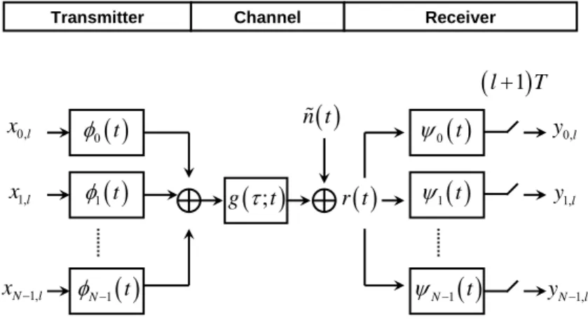
The continuous-time OFDM model presented in the Fig. 2-3 can be considered as the ideal baseband OFDM system model, which in practice is digitally synthesized and will be discussed in the next section. We start to introduce the continuous model with the waveforms used in the transmitter and proceed all the way to the receiver.

z Transmitter

Assumeing an OFDM system with N subcariers, a bandwidth of WHz and a

(27)

Transmitter Channel Receiver

( )

0 t φ

( )

1 t φ

( )

1 N t φ −

( )

; g τ t

( )

n t

( )

r t

( )

0 t ψ

( )

1 t ψ

( )

1 N t ψ −

(

l+1

)

T 0,l y 1,l y 1, N l y ₋ 0,l x 1,l x 1, N l x ₋

Fig. 2-3 Baseband OFDM system model

prefix, the transmitter uses the following waveforms

( )

[ ]

2 1 if 0, 0, otherwise g W j k t T N g k e t T T T t π φ − ⎧ ∈ ⎪ ₋ = ⎨ ⎪ ⎩ (2.7)

Where T =N W +Tg . Note that φk

( )

t =φk

(

t+N W

)

when t is within the cyclic prefix ⎡_⎣0,T_g⎤_{⎦ . Since}φ_k

( )

t is a rectangular pulse modulated on the carrier

frequency k W N , the common interpretation of OFDM is that it uses N

subcarriers, each carrying a low bit-rate. The waveforms φ_k

( )

t are used in the

modulation and the transmitted baseband signal for OFDM symbol number l as

( )

1 ,

(

)

0 N l k l k k s t x φ t lT − = =

∑

i − (2.8)

(28)

points. When an infinite sequence of OFDM symbols is transmitted, the output from the transmitter is a juxtaposition of individual OFDM symbols as

( )

1 ,

(

)

0 N l k l l l k s t s t x φ t lT ∞ ∞ − =−∞ =−∞ = =

∑

=

∑ ∑

− (2.9) z Physical channel

We assume that the support of the (possibly time variant) impulse response g

( )

τ,t

of the physical channel is restricted to the interval τ∈ ⎣⎡0,Tg⎤⎦ , i.e., to the length of the cyclic prefix. The received signal becomes

( ) (

)( )

( ) (

)

( )

0 ; g T r t = g s t× =

∫

g τ t s t−τ τd +n t (2.10)

Where n is additive, white, and complex Gaussian channel noise.

z Receiver

The OFDM receiver consists of a filter bank, matched to the last part ⎡⎣T Tg, ⎤⎦ of

the transmitter waveforms φ_k

( )

t , i.e.,

( )

(

)

if 0, , 0, otherwise. k g k T t t T T t φ ψ _{= ⎨}⎧⎪ ∗ − ∈⎡⎣ − ⎤⎦ ⎪⎩ (2.11)

Effectively this means that the cyclic prefix is removed in the receiver. Since the cyclic prefix contains all ISI from the precious symbol, the sampled output from the

(29)

receiver filter bank contains no ISI. Hence we can ignore the time index l when

calculating the sampled output at the _ th matched filter. By using (2.9), (2.10), and

(2.11), we get

(

)( )

( ) (

)

( )

(

)

( )

(

) ( )

1 ' ' ' 0 0 | ; g g g k k t T k T T N k k k k T T k T y r t r t T t dt g t x t d t dt n T t t dt ψ π ψ τ φ τ τ φ φ = ∞ −∞ − _∗ = ∗ = × = − ⎛ ⎞ ⎡ ⎤ = ⎜_⎜ _⎣ − _⎦ ⎟_⎟ ⎝ ⎠ + −

∫

∑

∫ ∫

∫

(2.12)

We consider the channel to be fixed over the OFDM symbol interval and denote it by g

( )

τ , which gives

( ) (

)

( )

(

) ( )

1 ' ' 0 0 g g g T T T N k k k k k _T _T y g τ φ t τ τ φd t dt n T t φ t dt − ∗ ∗ = ⎛ ⎞ = ⎜_⎜ − ⎟_⎟ + − ⎝ ⎠

∑ ∫ ∫

∫

(2.13)

The integration intervals are T_g < < and 0t T < <τ T_g , which implies that

0 t< − <τ T and the inner integral can be written as

( ) (

)

( )

( ) ( )

( )

' 0 2 ' 0 2 ' 2 ' 0 g g g g g T k T j k t T W N g T j k t T W N j k W N g g g t d e g d T T e g e d T t T T T π τ π π τ τ φ τ τ τ τ τ τ − − − − − = − = < < −

∫

(2.14)

(30)

The latter part of this expression is the sampled frequency response of the channel at frequency f =k W N' , i.e., at the kth subcarrier frequency:

( )

2 ' ' 0 ' g T j k W N k W h G k g e d N π τ τ − τ ⎛ ⎞ = _⎜ _⎟= ⎝ ⎠

∫

(2.15)

Where G f

( )

is the Fourier transform of g

( )

τ . Using this notation, the output

from the receiver filter bank can be simplified to

( )

(

) ( )

( ) ( )

2 ' 1 ' ' ' 0 1 ' ' ' ' 0 g g g g k j k t T W N T T N k k k k k T g T T N k k k k k k _T y e x h t dt n T t t dt T T x h t t dt n π φ φ φ φ − − ∗ ∗ = − ∗ = = + − − = +

∑ ∫

∫

∑

_∫

(2.16), where

(

) ( )

g T k _T k

n =

∫

n T−t φ∗ t dt. Since the transmitter filters φ_k

( )

t are orthogonal,

the following equation is thus obtained.

( ) ( )

[

]

' ' 2 ' 2 ' g g g g T k k T j k t T W N j k t T W N T T g g t t dt e e dt k k T T T T π π φ φ δ ∗ − − − = = − − −

∫

(2.17)

According to (2.16), we know that

k k k

(31)

0,l

x

1, N l

x

₋ 0,l

h

1, N l

h

₋ 0,l

n

1, N l

n

₋ 0,l

y

1, N l

y

₋

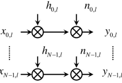
Fig. 2-4 Continuous-time OFDM system interpreted as parallel Gaussian channels.

The benefit of a cyclic prefix is twofold: it avoids both ISI (since it acts as a guard space) and ICI (since it maintains the orthogonality of the subcarriers). By re-introducing the time index

l, we may now view the OFDM system as a set of parallel Gaussian channels, according to

Fig. 2-4.

2.1.3 Discrete-Time Model

An entirely discrete-time model of and OFDM systme is displayed in Fig. 2-5. Compared to the continous-time model, the modulation and demodulation are replaced by an inverse DFT (IDFT) and a DFT respectively and the channel is a discrete-time convolution. The cyclic prefix operates in the same fashion in this system and the calculations can be performed in essentially the same way. The main difference is that all integrals are replaced by sums.

Transmitter Channel Receiver

IDFT 0,l x 1,l x 1, N l x − MUX CP

[ ]

s k

[

;

]

g m k

[ ]

n k

[ ]

r k CP DE MUX DF T 0,l y 1,l y 1, N l y ₋

(32)

As far as the receiver is concerned, the use of a cyclic prefix longer than the channel response will transform the linear convolution in the channel into a cyclic convolution. Denoting cyclic convolution by “⊗”, we can write the whole OFDM system as

( )

(

)

( )

(

)

l l l l l l

x

g

n

x

g

n

l

y

DFT IDFT

=

⊗ +

=

⊗

+

_(2.19)

Where y contains the _l N received data points, x is the _l N transmitted constellation

points, g is the channel impulse response of the channel (padded with zeros to obtain a length of N), and n is the channel noise. Since the channel noise is assumed to be white _l

Gaussian, the term n_l =DFT

( )

n_l represents uncorrelated Gaussian noise. Furthermore, we use the fact that the DFT of two cyclically convolved signals is equivalent to the product of their individual DFTs. Denoting element-by-element multiplication by “ i ”, the above expression can thus be written as

( )

l l l l l l l

y

=

x

i

DFT

g

+

n =x h +n

i

(2.20)

Where h_l =DFT

( )

g_l is the frequency response of the channel. Therefore we have

obtained the same type of parallel Gaussian channels as the continuous-time model. The only difference is that the channel attenuations h are given by the _l N -point DFT of the

(33)

2.1.4 Imperfections of OFDM

Depending on the mathematical analyzed situation disscused before, imperfections in a real OFDM system may be ignored or explicitly included in the model. Below we mention of the imperfections and their corresponding effects.

z Dispersion

Both time and frequency dispersion of the channel can destroy the orthogonality of the system, i.e., introduce both ISI and ICI. If these effects are not sufficiently mitigated by e.g., a cyclic prefix and a large inter-carrier spacing, they have to be included in the model. One way of modelling these effects is an increase of the additive noise.

z Nonlinearities and clipping distortion

OFDM systems have high peak-to-average power ratios and high demands on linear amplifiers. Nonlinearities in amplifiers may cause both ISI and ICI in the system. Especially, if the amplifiers are not designed with proper output back-off (OBO), the clipping distortion may cause severe degradation.

z External interference

In wireless systems, the external interference usually stems from radio transmitters and other types of electronic equipment in the vinciniy of the receiver.

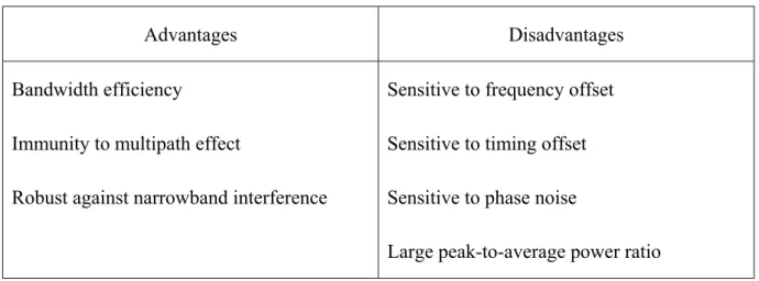
2.2 Introduction to OFDMA

(34)

Table 2-1 OFDM Advantages and Disadvantages

Advantages Disadvantages

Bandwidth efficiency

Immunity to multipath effect

Robust against narrowband interference

Sensitive to frequency offset Sensitive to timing offset Sensitive to phase noise

Large peak-to-average power ratio

transmissions to and from multiple users along with the other advantages of OFDM. In OFDM, a channel is divided into carriers which is used by one user at any time. In OFDMA, the carriers are divided into subchannels. Each subchannel has multiple carriers that form one unit in frequency allocation. In this way, the bandwidth can be allocated dynamically to the users according to their needs. A simple comparison of the subcarrier allocation of OFDM

(35)

and OFDMA is shown in Fig. 2-6.

An additional advantage of OFDMA is the following. Due to the large variance in a mobile system’s path loss, inter-cell interference is a common issue in mobile wireless systems. An OFDMA system can be designed such that subchannels can be composed from several distinct permutations of subcarriers. This enables significant reduction in inter-cell interference when the system is not fully loaded, because even on occasions where the same subchannel is used at the same time in two different cells, there is only a partial collision on

(36)

the active sub-carriers.

Fig. 2-7 shows an example subcarrier allocation in an OFDMA symbol. The frequency response of a typical broadband wireless channel is also depicted. In this example, the deep-fading condition and narrowband interference are considered. In the top plot, we see that when the channel is in deep fade, the subcarriers are not sufficiently energy efficient to carry information. These wasted subcarriers can be utilized by there uses in OFDMA, thus achieving higher efficiency and capacity. Very few, if any, subcarriers are likely to be wasted in OFDMA, since no particular subcarrier is likely to be bad for all users.

In order to support multiple users, the control mechanism becomes more complex. Besides, the OFDMA system has some implementation issues which are more complicated to handle. For example, power control is needed for the uplink to make signals from different users have equal power at the receiver, and all users have to adjust their transmitting time to be aligned. We shall address some issues in the context of IEEE 802.16e.

2.3 Introduction to

IEEE 802.16e

Since the publication of the IEEE 802.16 standard for fixed broadband wireless access in 2001, a number of revision and amendments have taken place. Like other IEEE 802 standards, the 802.16 standards are primarily concerned with physical (PHY) layer and medium access control (MAC) layer functionalities. The idea originally was to provide broadband wireless access to buildings through external antennas communicating with radio base stations (BSs).

(37)

transmitters and receivers in the 802.16 standard, the 802.16a standard was approved in 2003 to support nonline-of-sight (NLOS) links, operational in both licensed and unlicensed frequency bands from 2 to 11 GHz, and subsequently revised to create the 802.16d standard (now code-named 802.16-2004). With such enhancements, the 802.16-2004 standard has been viewed as a promising alternative for providing the last-mile connectivity by radio link. However, the 802.16-2004 specifications were devised primarily for fixed wireless users. The 802.16e task group was subsequently formed with the goal of extending the 802.16-2004 standard to support mobile terminals.

The IEEE 802.16e has been published in Febuary 2006. It specifies four air interfaces: WirelessMAN-SC PHY, WirelessMAN-SCa PHY, WirelessMAN-OFDM PHY, and WirelessMAN-OFDMA PHY. This study is concerned with WirelessMAN-OFDMA PHY in a mobile communication environment.

Some glossary we will often use in the following is as follows. The direction of transmission from the base station (BS) to the subscriber station (SS) is called downlink (DL), and the opposite direction is uplink (UL). The SS is considered synonymous as the mobile station (MS). It is sometimes termed the user. The BS is a generalized equipment set providing connectivity, management, and control of the SS.

2.3.1 OFDMA Basic Terms

In the OFDMA mode, the active subcarriers are divided into subsets of subcarriers, where each subset is termed a subchannel. The subcarriers forming one subchannel may, but need

(38)

Fig. 2-8 OFDMA frequency description (3-channel schematic example, from [4]).

not be, adjacent. The concept is shown in Fig. 2-8.

Three basic types subchannel organization are defined: partial usage of subchannels (PUSC), full usage of subchannels (FUSC), and adaptive modulation and coding (AMC); among which the PUSC is mandatory and the other two are optional. In PUSC DL, the entire channel bandwidth is divided into three segments to be used separately. The FUSC is employed only in the DL and it uses the full set of available subcarriers so as to maximize the throughput.

Slot and Data Region

The definition of an OFDMA slot depends on the OFDMA symbol structure, which varies for uplink and downlink, for FUSC and PUSC, and for the distributed subcarrier permutations and the adjacent subcarrier permutation.

z For downlink PUSC using the distributed subcarrier permutation, one slot is one subchannel by two OFDMA symbols.

z For uplink PUSC using either of the distributed subcarrier permutations, one slot is

one subchannel by three OFDMA symbols.

z For downlink FUSC and downlink optional FUSC using the distributed subcarrier

permutation, one slot is one subchannel by one OFDMA symbol.

(39)

Fig. 2-9 Example of the data region which defines the OFDMA allocation (from [4]).

subchannels, in a group of contiguous OFDMA symbols. All the allocations refer to logical subchannels. This two-dimensional allocation may be visualized as a rectangle, such as the

4 3× rectangle shown in Fig. 2-9

Segment

A segment is a subdivision of the set of available OFDMA subchannels (that may include all available subchannels). One segment is used for deploying a single instance of the MAC.

Permutation Zone

A permutation zone is a number of contiguous OFDMA symbols, in the DL or the UL, that use the same permutation formula. The DL subframe or the UL subframe may contain more than one permutation zone. The concept of permutation zone will be further elaborate later.

2.3.2 OFDMA Symbol Parameters

z Some OFDMA symbol parameters are listed below.

z BW: Nominal channel bandwidth. z N_used: Number of used subcarriers.

z n: Sampling factor. This parameter, in conjunction with BW and N_used, determines the subcarrier spacing and the useful symbol time.

(40)

z G: Ratio of cyclic prefix (CP) time to useful time. z N_FFT : Smallest power of two greater than N_used. z Sampling frequency: Fs = ⋅

[

n BW 8000 800

]

× .

z Subcarrier spacing: Δ =f F Ns FFT . z Useful symbol time: T_b = Δ .1 f z Cyclic prefix (CP) time: T_g = ⋅ .G T_b z OFDM symbol time: Ts = + .Tb Tg z Sampling time: T N_b _FFT .

2.3.3 Scalable OFDMA [9]

One feature of the IEEE 802.16e OFDMA is the selectable FFT size, from 128 to 2048 in multiples of 2, excluding 256 to be used with OFDM. This has been termed scalable OFDMA (S-OFDMA). One use of S-OFDMA is that if the channel bandwidths are allocated based on integer power of 2 times a base bandwidth, then one may consider making the FFT size proportional to the allocated bandwidth so that all systems are based on the same subcarrier spacing and the same OFDMA symbol duration, which may simplify system design. For example, Table 2-2 lists some S-OFDMA parameters proposed by the WiMAX Forum [10]. S-OFDMA supports a wide range of bandwidth to flexibly address the need for various spectrum allocation and usage model requirements.

When designing OFDMA wireless systems the optimal choice of the number of subcarriers per channel bandwidth is a tradeoff between protection against multipath, Doppler shift, and design cost/coplexity. Increasing the number of subcarriers leads to better immunity to the ISI

(41)

Table 2-2 S–OFDMA Parameters Proposed by WiMAX Forum

Parameters

Values

System Channel Bandwidth (MHz) 1.25 5 10 20

Sampling Frequency (MHz) 1.4 5.6 11.2 22.4

FFT Size 128 512 1024 2048

Subcarrier Spacing ( fΔ ) 10.94 kHz

Useful Symbol Time(T_b = Δ )1 f 91.4 μ sec

Guard Time(T_g =T_b 8) 11.4 μ sec

OFDMA Symbol Duration(Ts = + )Tb Tg 102.9 μsec

caused by multipath; on the other hand it increases the cost and complexity of the system (it leads to higher requirements for signal processing power and power amplifiers with the capability of handling higher peak-to-average power ratios). Having more subcarriers also results in narrower subcarrier spacing and therefore the system becomes more sensitive to Doppler shift and phase noise. Calculations show that the optimum tradeoff for mobile systems is achieved when subcarrier spacing is about 11 kHz [11] .

2.4 OFDMA Frame Structure

Duplexing Modes

In licensed bands, the duplexing method shall be either frequency-division duplex (FDD) or time-division duplex(TDD). FDD SSs may be half-duplex FDD (H-FDD). In license exempt bands, the duplexing method shall be TDD.

Point-to-Multipoint (PMP) Frame Structure

When implementing a TDD system, the frame is composed of BS and SS transmissions. Fig. 2-10 shows an example. Each frame in the downlink transmission begins with a preamble

(42)

Fig. 2-10 Example of an OFDMA frame (with only mandatory zone) in TDD mode (from [2]).

followed by a DL transmission period and an UL transmission period. In each frame, time gaps, denoted transmit/receive transition gap (TTG) and receive/transmit gap (RTG), are between the downlink and uplink subframes and at the end of each frame, respectively placed. They allow transitions between transmission and reception functions.

Subchannel allocation in the downlink may be performed with PUSC where some of the subchannels are allocated to the transmitter or FUSC where all subchannels are allocated to the transmitter. The downlink frame shall start in PUSC mode with no transmit diversity. The FCH shall be transmitted using QPSK rate 1/2 with four repetitions using the mandatory coding scheme (i.e., the FCH information will be sent on four subchannels with successive logical subchannel numbers) in a PUSC zone. The FCH contains the DL Frame Prefix which specifies the length of the DL-MAP message that immediately follows the DL Frame Prefix

(43)

Fig. 2-11 Illustration of OFDMA with multiple zones (from [2]).

and the repetition coding used for the DL-MAP message.

The transitions between modulations and coding take place on slot boundaries in time domain (except in AAS zone, where AAS stands for adaptive antenna system) and on subchannels within an OFDMA symbol in frequency domain. The OFDMA frame may include multiple zones (such as PUSC, FUSC, PUSC with all subchannels, optional FUSC, AMC, TUSC1, and TUSC2, where AMC stands for adaptive modulation and coding, and TUSC stands for tile usage of subchannels), the transition between zones is indicated in the DL-Map. Fig. 2-11 depicts an OFDMA frame with multiple zones.

The PHY parameters (such as channel state and interference levels) may change from one zone to the next.

The maximum number of downlink zones is 8 in one downlink subframe. For each SS, the maximum number of bursts to decode in one downlink subframe is 64. This includes all bursts without connection identifier (CID) or with CIDs matching the SS’s CIDs.

Allocation of Subchannels for FCH and DL-MAP, and Logical Subchannel Numbering

(44)

Fig. 2-12 FCH subchannel allocation for all 3 segments (from [4]).

subchannel group #0. For FFT sizes other than 128, the first 4 slots in the downlink part of the segment contain the FCH as defined before. These slots contain 48 bits modulated by QPSK with coding rate 1/2 and repetition coding of 4. For FFT-128, the first slot in the downlink part of the segment is dedicated to FCH and repetition is not applied. The basic allocated subchannel sets for segments 0, 1, and 2 are subchannel groups #0, #2, and #4, respectively. Fig. 2-12 depicts this structure.

After decoding the DL Frame Prefix message within the FCH, the SS has the knowledge of how many and which subchannels are allocated to the PUSC segment. In order to observe the allocation of the subchannels in the downlink as a contiguous allocation block, the subchannels shall be renumbered. The renumbering, for the first PUSC zone, shall start from the FCH subchannels (renumbered to values 0–11), then continue numbering the subchannels in a cyclic manner to the last allocated subchannel and from the first allocated subchannel to the FCH subchannels. Fig. 2-13 gives an example of such renumbering for segment 1.

(45)

Fig. 2-13 Example of DL renumbering the allocated subchannels for segment 1 in PUSC(from [4]).

For uplink, in order to observe the allocation of the subchannels as a contiguous allocation block, the subchannels shall be renumbered, and the renumbering shall start from the lowest numbered allocated subchannel (renumbered to value 0), up to the highest numbered allocated subchannel, skipping nonallocated subchannels.

The DL-MAP of each segment shall be mapped to the slots allocated to the segment in a frequency first order, starting from the slot after the FCH (subchannel 4 in the first symbol, after renumbering), and continuing to the next symbols if necessary. The FCH of segments that have no subchannels allocated (unused segments) will not be transmitted, and the respective slots may be used for transmission of MAP and data of other segments.

2.5 OFDMA Subcarrier Allocation

(46)

For convenience, here we only take the 1024-FFT OFDMA subcarrier allocation for introduction. The subcarriers are divided into three types: null (guard band and DC), pilot, and data. Subtracting the guard tones from NFFT , one obtains the set of “used” subcarriers Nused. For both uplink and downlink, these used subcarriers are allocated to pilot subcarriers and data subcarriers. However, there is a difference between the different possible zones. For FUSC and PUSC, in the downlink, the pilot tones are allocated first; what remains are data subcarriers, which are divided into subchannels that are used exclusively for data. Thus, in FUSC, there is one set of common pilot subcarriers, and in PUSC downlink, there is one set of common pilot subcarriers in each major group, but in PUSC uplink, each subchannel contains its own pilot subcarriers.

2.5.1 Downlink

Preamble

The first symbol of the downlink transmission is the preamble. There are three types of preamble carrier-sets, which are defined by allocation of different subcarriers for each one of them. The subcarriers are modulated using a boosted BPSK modulation with a specific pseudo-noise (PN) code. The preamble carrier-sets are defined using

PreambleCarrierSetn=n+ ⋅3 k (2.21)

Where :

PreambleCarrierSetn specifies all subcarriers allocated to the specific preamble,

n is the number of the preamble carrier-set indexed 0–2,

(47)

For the preamble symbol there are 86 guard band subcarriers on the left side and the right side of the spectrum. Each segment uses a preamble composed of a carrier-set out of the three available carrier-sets in the manner that segment i uses preamble carrier-set i, where i = 0, 1, 2. Therefore, each segment eventually modulates each third subcarrier. In the case of segment 0, the DC carrier will be zeroed and the corresponding PN number will be discarded.

The 114 different PN series modulating the preamble carrier-set are defined in Table 309 of [4] for the 1024-FFT mode. The series modulated depends on the segment used and the IDcell parameter.

Symbol Structure for PUSC

The symbol is first divided into basic clusters and zero carriers are allocated. Pilots and data

carriers are allocated within each cluster. Table 310 of [2] summarizes the parameters of the symbol structure of different FFT sizes for PUSC mode. Here we only take the 1024-FFT OFDMA downlink carrier allocation for example, which is summarized in Table 2-3. Fig. 2-14 depicts the DL cluster structure.

Downlink Subchannels Subcarrier Allocation in PUSC

The subcarrier allocation to subchannels is performed using the following procedure:

1. Dividing the subcarriers into the number of clusters (Nclusters), where the physical clusters

(48)

Table 2-3 1024-FFT OFDMA DL Carrier Allocation for PUSC

Parameter Value Comments

Number of DC subcarriers 1 Index 512

Number of guard subcarriers, left 92

Number of guard subcarriers, right 91

Number of used subcarriers, N_used 841

Renumbering sequence 6, 48, 37, 21, 31, 40, 42, 56, 32, 47, 30, 33, 54, 18, 10, 15, 50, 51, 58, 46, 23, 45, 16, 57, 39, 35, 7, 55, 25, 59, 53, 11, 22, 38, 28, 19, 17, 3, 27, 12, 29, 26, 5, 41, 49, 44, 9, 8, 1, 13, 36, 14, 43, 2, 20, 24, 52,4, 34, 0

Used to renumber clusters before allocation to subchannels.

Number of subcarriers per cluster 14

Number of clusters 60

Number of data subcarriers in each symbol per subchannel

24

Number of subchannels 30

Basic permutation sequence 6 (for 6 subchannels)

3, 2, 0, 4, 5, 1

Basic permutation sequence 4 (for 4 subchannels)

3, 0, 2, 1

contain 14 adjacent subcarriers each (starting from carrier 0). The number of clusters varies with the FFT size.

(49)

=

first DL zone, or Use All SC indicator = 0 in STC DL Zone IE, LogicalCluster RenumberingSequence(PhysicalCluster) , Renumbe otherwise. clusters ringSequence((PhysicalCluster)+ 13 DL PermBase)modN ⎧ ⎪ ⎪⎪ ⎨ ⎪ ⎪ ⋅ ⎪⎩ (2.22)

In the first PUSC zone of the downlink (first downlink zone) and in a PUSC zone defined by STC DL ZONE IE() with “use all SC indicator = 0”, the default renumbering sequence is used for logical cluster definition. For all other cases DL PermBase parameter in the STC DL Zone IE() or AAS DL IE() shall be used.

3. Allocating logical clusters to groups. The allocation algorithm varies with FFT size. For FFT size = 1024, dividing the clusters into six major groups. Group 0 includes clusters 0–11, group 1 clusters 12–19, group 2 clusters 20–31, group 3 clusters 32–39, group 4 clusters 40–51, and group 5 clusters 52–59. These groups may be allocated to segments; if a segment is used, then at least one group shall be allocated to it. By default group 0 is allocated to sector 0, group 2 to sector 1, and group 4 to sector 2.

4. Allocating subcarriers to subchannels in each major group, which is performed separately for each OFDMA symbol by first allocating the pilot carriers within each cluster, and then partitioning all remaining data carriers into groups of contiguous subcarriers. Each subchannel consists of one subcarrier from each of these groups. The number of groups is therefore equal to the number of subcarriers per subchannel, and it is denoted Nsubcarriers. The number of the subcarriers in a group is equal to the number of subchannels, and it is denoted Nsubchannels. The number of data subcarriers is thus equal to

subcarriers subchannels

(50)

parameters from Table 2-3, with basic permutation sequence 6 for even numbered major groups and basic permutation sequence 4 for odd numbered major groups, to partition the subcarriers into subchannels containing 24 data subcarriers in each symbol. The exact partitioning into subchannels is according to the permutation formula:

( )

[

]

{

}

, mod _ mod subchannels k s k subchannels subchannels subcarrier k s N n p n N DL PermBase N = ⋅ + + (2.23) where:

( )

,

subcarrier k s is the subcarrier index of subcarrier k in subchannel s,

s is the index number of a subchannel, from the set

{

0,...,N_subchannels−1

}

,

k

n =

(

k+ ⋅13 s

)

mod N_subchannelswhere k is the subcarrier-in-subchannel index

from the set

{

0,...,Nsubchannels −1

}

,

subchannels

N is the number of subchannels (for PUSC use number of subchannels in the currently partitioned major group),

[ ]

s

p j is the series obtained by rotating basic permutation sequence cyclically to

the left s times, _

DL PermBase is an integer ranging from 0 to 31, which is set to the preamble IDCell in the first zone and determined by the DL-MAP for other zones.

On initialization, an SS must search for the downlink preamble. After finding the preamble, the user shall know the IDcell used for the data subchannels.

2.5.2 Uplink

(51)

Table 2-4 1024-FFT OFDMA UL Carrier Allocation for PUSC

Parameter Value Comments

Number of DC subcarriers 1 Index 512

Nused 841

Guard subcarriers: left, right 92,91

TilePermutation 11, 19, 12, 32, 33, 9, 30, 7, 4, 2, 13, 8, 17, 23, 27, 5, 15, 34, 22, 14, 21, 1, 0, 24, 3, 26, 29, 31, 20, 25, 16, 10, 6, 28, 18

used to allocate tiles to subchannels

Nsubchannels 35

Ntiles 210

Tile per subchannel 6

supports 35 subchannels where each transmission uses 48 data subcarriers as the minimal block of processing. Each new transmission for the uplink commences with the parameters as given in Table 2-4.

Symbol Structure for Subchannel (PUSC)

A slot in the uplink is composed of three OFDMA symbols and one subchannel. Within each slot, there are 48 data subcarriers and 24 fixed-location pilots. The subchannel is constructed from six uplink tiles, each tile has four successive active subcarriers and its configuration is illustrated in Fig. 2-15 .

(52)

Partitioning of Subcarriers into Subchannels in the Uplink

The usable subcarriers in the allocated frequency band shall be divided into Ntiles physical tiles as defined in Fig. 2-15 with parameters from Table 2-4. The allocation of physical tiles to logical tiles in subchannels is performed in the following manner:

( )

(

)

{

}

, mod _ mod subchannels k t subchannels subchannels Tiles s n N n p s n N UL PermBase N = ⋅ + ⎡_⎣ + ⎤_⎦+ (2.24) where:

( )

,

Tiles s n is the physical tile index in the FFT with tiles being ordered consecutively

from the most negative to the most positive used subcarrier (0 is the starting tile index),

n is the tile index 0,...,5 in a subchannel,

t

p is the tile permutation,

subchannels

N is the number of subchannels,

s is the subchannel number in the range

{

0,...,N_subchannels−1

}

_

UL PermBase is an integer value in the range 0:::69, which is assigned by a management entity.

After mapping the physical tiles in the FFT to logical tiles for each subchannel, the data subcarriers per slot are enumerated by the following process:

1. After allocating the pilot carriers within each tile, indexing of the data subcarriers within each slot is performed starting from the first symbol at the lowest indexed subcarrier of

(53)

the lowest indexed tile and continuing in an ascending manner through the subcarriers in the same symbol, then going to the next symbol at the lowest indexed data subcarrier, and so on. Data subcarriers shall be indexed from 0 to 47.

2. The mapping of data onto the subcarriers will follow (2.25), which calculates the subcarrier index (as assigned in item 1) to which the data constellation point is to be mapped:

( ) (

, 13

)

mod _subchannels

Subcarriers n s = n+ ⋅s N (2.25)

where:

( )

,

Subcarriers n s is the permutated subcarrier index corresponding to data subcarrier n is

subchannel s,

n is the running index 0,...,47, indicating the data constellation point, s is the subchannel number,

subchannels

N is the number of subcarriers per slot.

2.6 Modulation

Subcarrier Randomization

The pseudo random binary sequence (PRBS) generator, as shown in Fig. 2-16, shall be used to produce a sequence w . The polynomial for the PRBS generator shall be k

11 9 ₁

X +X + . The value of the pilot modulation on subcarrier k shall be derived from w ._k

The initialization vector of the PRBS generator for both uplink and downlink, designated b10..b0, is defined as follows:

b0..b4 = five least significant bits of IDcell as indicated by the frame preamble in the first downlink zone and in the downlink AAS zone with Diversity Map support, DL PermBase

(54)

Fig. 2-16 PRBS generator for pilot modulation (from [2]).

following STC DL Zone IE() and 5 LSB of DL PermBase following AAS DL IE without Diversity Map support in the downlink. Five least significant bits of IDcell (as determined by the preamble) in the uplink. For downlink and uplink, b0 is MSB and b4 is LSB, respectively. b5..b6 = set to the segment number + 1 as indicated by the frame preamble in the first downlink zone and in the downlink AAS zone with Diversity Map support, PRBS ID as indicated by the STC DL Zone IE or AAS DL IE without Diversity Map support in other downlink zone. 0b11 in the uplink. For downlink and uplink, b5 is MSB and b6 is LSB, respectively.

b7..b10 = 0b1111 (all ones) in the downlink and four LSB of the Frame Number in the uplink. For downlink and uplink, b7 is MSB and b10 is LSB, respectively.

Data Modulation

After the repetition block, the data bits are entered serially to the constellation mapper. Gray-mapped QPSK and 16-QAM shall be supported, whereas the support of 64-QAM is optional.

Pilot Modulation

In all permutations except uplink PUSC and downlink TUSC1, each pilot shall be transmitted with a boosting of 2.5 dB over the average non-boosted power of each data tone. The pilot

(55)

subcarriers shall be modulated according to

{ }

8 1 ,

{ }

0, 3 2 k k k k c ⎛ w ⎞ p c ℜ = _⎜ − _⎟⋅ ℑ = ⎝ ⎠ (2.26)

where p _k is the pilot’s polarity for SDMA (spatial division multiple access) allocations in AMC AAS zone, and p = 1 otherwise.

Preamble Pilot Modulation

The pilots in the downlink preamble shall be modulated according to

{

}

4 2 1 2 k PreambleP ilotModulation ⎛ w ⎞ ℜ = ⋅ ⋅_⎜ − _⎟ ⎝ ⎠ (2.27)

{

PreambleP ilotModulation

}

0. ℑ = (2.28)

2.7 Transmit Spectral Mask

Due to requirement of bandwidth-limited transmission, the transmitted spectral density of the transmitted signal shall fall within the spectral mask as shown in Fig. 2-17 and Table 2-5 in license-exempt bands. The measurements shall be made using 100 kHz resolution bandwidth and a 30 kHz video bandwidth. The 0 dBr level is the maximum power allowed by the relevant regulatory body. IEEE 802.16e dose not specify the power mask for the licensed bands.

Table 2-5 Transmit Sprctral Mask for License-Exempt Bands

Bandwidth (MHz)

A B C D

10 9.5 10.9 19.5 29.5

(56)

Fig. 2-17 Transmit spectral mask for license-exempt operation (from[4]).

2.8 Frequency and Timing Requirements

Timing Requirements

For any duplexing, all SSs shall acquire and adjust their timing such that all uplink OFDMA symbols arrive time coincident at the BS to an accuracy of ±25% of the minimum guard interval or better. For example, this translates into ±8 samples in the case of 1024-FFT OFDMA.

Frequency Requirements

At the BS, the transmitted center frequency, receive center frequency, and the symbol clock frequency shall be derived from the same reference oscillator. At the BS, the reference frequency accuracy shall be better than _{± ×}_{2 10}−6_.

At the SS, both the transmitted center frequency and the sampling frequency shall be derived from the same reference oscillator. Thereby, the SS uplink transmission shall be locked to the

(57)

BS, so that its center frequency shall deviate no more than 2% of the subcarrier spacing, compared to the BS center frequency.

During the synchronization period, the SS shall acquire frequency synchronization within the specified tolerance before attempting any uplink transmission. During normal operation, the SS shall track the frequency changes by estimating the downlink frequency offset and shall defer any transmission if synchronization is lost. To determine the transmit frequency, the SS shall accumulate the frequency offset corrections transmitted by the BS (for example in the RNG-RSP message), and may add to the accumulated offset an estimated UL frequency offset based on the downlink signal.

(58)

Chapter 3 Decision Directed

Channel Estimation

This section describes some channel estimation schemes to deal with different environments. After finding the packet starting point, channel estimation is performed to recover the channel frequency response. In this Chapter, the channel estimation will be introduced in detail. Then, we give a brief overview of the relevant technique.

3.1 Channel Estimation Structure

The simple structure of the channel estimation is show as Fig. 3-1. The received signal is modeled as Y m

( )

=H m X m

( ) ( )

+N m

( )

, Y is the received signal, X is QPSK i.i.d.

transmitted signal, H is with zero mean complex Gaussian distribution, N is white

Gaussian noise, and m is subcarrier index.

Rx_signal Initial Channel Iteration-Decision directed Final result

ˆH

H

Y

(59)

There are two operations in the structure. One is the initial channel response estimation, the other is the iteration steps to refine the channel response until convergence.

3.2 Obtain The Initial Channel

We have some different choices to obtain the initial channel responses, namely, Pilot Symbol Aided, Linear Prediction, and Linear Interpolation.

Pilot Symbol Aided [17][18]

We add pilots X_Np to a symbol block. Denote N as the pilot numbers, and _p reasonably assume pilots X_Np are known. We can obtain the initial channel H_Np, then put the initial channel H_Np into a low pass filter. The output of the low pass filter is the final result ˆH .

Linear Prediction [15][16]

Suppose the last p s symbol channels are known perfectly, we predict the ' p+ 1 channel from the previous 1 ~ p channels.

Linear Interpolation

We need a buffer to save a block of data. We use Pilot Symbol Aided in the first and last symbol to obtain channel, and the initial channels of the other symbols are obtained by the Linear Interpolation.

3.2.1 Pilot Symbol Aided

(60)

pilot data Time Sub -ca rr ier pilot pilot pilot

Fig. 3-2 Pilot Symbol Aided

fading channel requires constant tracking, so pilot information has to be transmitted more or less continuously. Decision-directed channel estimation can also be used. But even in these types of schemes, pilot information has to be transmitted regularly to mitigate error propagation. The structure of the Pilot Symbol Aided is show as the Fig. 3-2. The channel of every symbol was estimated by pilot. The initial channel estimation of every symbol was shown in the follow description,

( ) ( )

(

)

[ ] , ,0 1 H [0] , where is others Np Y m X m m i M Np i Np m = ≤ ≤ − ⎧⎪ = ⎨ ⎪⎩ (3.1)

The illustration is shown in Fig. 3-3

( )

0 H

( )

H m m 0 1 2 m M−1 0 0 0 0 0 0 0 0 0

移動WiMAX系統之導引碼輔助疊代式通道估測

國

立

交

通

大

學

電子工程學系 電子研究所碩士班

碩

士

論

文