Analysis and complexity reduction of multiple reference frames motion estimation in H.264/AVC

Analysis and Complexity Reduction of Multiple

Reference Frames Motion Estimation in H.264/AVC

Yu-Wen Huang

,

Bing-Yu Hsieh

,

Shao-Yi Chien, Member

,

Shyh-Yih Ma

, and

Liang-Gee Chen, Fellow

Abstract—In the new video coding standard H.264/AVC, motion estimation (ME) is allowed to search multiple reference frames. Therefore, the required computation is highly increased, and it is in proportion to the number of searched reference frames. However, the reduction in prediction residues is mostly dependent on the nature of sequences, not on the number of searched frames. Sometimes the prediction residues can be greatly reduced, but frequently a lot of computation is wasted without achieving any better coding performance. In this paper, we propose a con-text-based adaptive method to speed up the multiple reference frames ME. Statistical analysis is first applied to the available information for each macroblock (MB) after intra-prediction and inter-prediction from the previous frame. Context-based adaptive criteria are then derived to determine whether it is necessary to search more reference frames. The reference frame selection cri-teria are related to selected MB modes, inter-prediction residues, intra-prediction residues, motion vectors of subpartitioned blocks, and quantization parameters. Many available standard video sequences are tested as examples. The simulation results show that the proposed algorithm can maintain competitively the same video quality as exhaustive search of multiple reference frames. Meanwhile, 76%–96% of computation for searching unnecessary reference frames can be avoided. Moreover, our fast reference frame selection is orthogonal to conventional fast block matching algorithms, and they can be easily combined to achieve further efficient implementations.

Index Terms—ISO/IEC 14496-10 AVC, ITU-T Rec. H.264, JVT, motion estimation (ME), multiple reference frames.

I. INTRODUCTION

E

XPERTS from ITU-T Video Coding Experts Group (VCEG) and ISO/IEC Moving Picture Experts Group (MPEG) formed the Joint Video Team (JVT) in 2001 to de-velop a new video coding standard, H.264/AVC [1]. Compared with MPEG-4 [2], H.263 [3], and MPEG-2 [4], the new stan-dard can achieve 39%, 49%, and 64% of bit-rate reduction, respectively [5]. The functional blocks of H.264/AVC, as well as their features, are shown in Fig. 1. Like previous standards, H.264/AVC still uses motion compensated transform coding.

Manuscript received May 22, 2003; revised July 10, 2005. This paper was recommended by Associate Editor S.-U. Lee.

Y.-W. Huang and B.-Y. Hsieh were with the Department of Electrical Engineering II, National Taiwan University, Taipei 10617, Taiwan, R.O.C. They are now with MediaTek, Inc., Hsinchu 300, Taiwan, R.O.C. (e-mail: yuwen@video.ee.ntu.edu.tw; BY_Hsieh@mtk.com.tw).

S.-Y. Chen and L.-G. Chen are with the Department of Electrical En-gineering II, National Taiwan University, Taipei 10617, Taiwan, R.O.C. (e-mail: shoayi@video.ee.ntu.edu.tw; steve@vivotek.com; lgchen@video. ee.ntu.edu.tw).

S.-Y. Ma is with Vivotek Inc., Taiwan, R.O.C. (e-mail: steve@vivotek.com) Digital Object Identifier 10.1109/TCSVT.2006.872783

The improvement in coding performance comes mainly from the prediction part. Motion estimation (ME) at quarter-pixel ac-curacy with variable block sizes and multiple reference frames greatly reduces the prediction errors. Even if inter-frame pre-diction cannot find a good match, intra-prepre-diction will make it up instead of directly coding the texture as before.

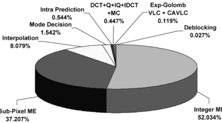
The reference software of H.264/AVC, JM [6], adopts full search for both motion estimation (ME) and intra-prediction. The instruction profile of the reference software on Sun Blade 1000 with UltraSPARC III 1 GHz CPU shows that real-time encoding of CIF 30 Hz video (baseline options, search range [ 16.75, 16.75], five reference frames) requires 314 994 million instructions per second and memory access of 471 299 Mbytes/s. The run time percentage of each function is shown in Fig. 2. Apparently, ME is the most computationally intensive part. In H.264/AVC, although there are seven kinds of block size (16 16, 16 8, 8 16, 8 8, 8 4, 4 8, 4 4) for motion compensation (MC), the complexity of ME in the refer-ence software is not seven times of that for one block size. The search range centers of the seven kinds of block size are all the same, so that the sum of absolute difference (SAD) of a 4 4 block can be reused for the SAD calculation of larger blocks. In this way, variable block size ME does not lead to much increase in computation. Intra-prediction allows four modes for 16 16 blocks and nine modes for 4 4 blocks. Its complexity can be estimated as the SAD calculation of 13 16 16 blocks plus extra operations for interpolation, which are relatively small compared with ME. As for the multiple reference frames ME, it contributes to the heaviest computational load. The required operations are proportional to the number of searched frames. Nevertheless, the decrease in prediction residues depends on the nature of sequences. Sometimes the prediction gain by searching more reference frames is very significant, but usually a lot of computation is wasted without any benefits.

In this paper, an effective method for accelerating the multiple reference frames ME without significant loss of video quality is proposed. The available information after intra-prediction and ME from the previous frame is first analyzed. Then we decide to keep on searching one more reference frame or to terminate the block matching process in the early stage. The rest of this paper is organized as follows. In Section II, the related back-ground including the flow of macroblock (MB) mode decision in the reference software and our modifications is reviewed. In Section III, we first analyze the statistics of selected MB modes, inter-prediction residues, intra-prediction residues, mo-tion vector (MVs) of subpartimo-tioned blocks, and quantizamo-tion parameter (QP). Then we propose our fast algorithm in Sec-tion IV. SimulaSec-tion results will be shown in SecSec-tion V. Finally, Section VI gives a conclusion.

Fig. 1. Functional blocks and features of H.264.

Fig. 2. Runtime percentages of functional blocks in H.264/AVC baseline en-coder.

II. FUNDAMENTALS

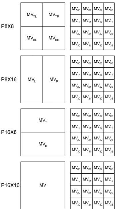
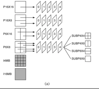
Fig. 3(a) illustrates the prediction part in the reference soft-ware baseline encoder. The prediction of a MB is performed mode by mode with full search scheme. There are four inter-MB modes (P8X8, P8X16, P16X8, and P16X16) and two intra-MB modes (I4MB and I16MB). Each 8 8 block of the P8X8 mode can be further subpartitioned into smaller blocks (SUBP4 4, SUBP4 8, SUBP8 4, and SUBP8X8), and the subparti-tioned blocks in an 8 8 block must be predicted from the same reference frame. The best MB mode is chosen by consid-ering a Lagrangian cost function, which includes both distortion and rate (number of bits required to code the side information). Let the QP and the Lagrange parameter (a QP-depen-dent variable) be given. The Lagrangian mode decision for a MB

proceeds by minimizing

(1) where the MB mode is varied over all possible coding modes. Experimental selection of Lagrangian multipliers is discussed in [7] and [8]. Fig. 3(b) shows the pseudocodes of MB mode decision in the reference software baseline encoder. It is clear that the outer loop is for MB modes, and the loops for refer-ence frames are inner. At the beginning of mode decision, SADs of the 16 4 4 blocks of a MB are calculated at all integer search positions in all reference frames. These SAD values can be reused for other blocks of larger sizes because their search range centers are exactly the same. When computing the La-grangian cost of integer search positions, the reference software uses the SAD value as the distortion part. After the best integer search position is found, the Lagrangian costs of the surrounding eight half-search positions are computed, and then again the La-grangian costs of eight quarter-search positions surrounding the best half-search position are computed. For fractional pixel ME, the reference software allows users to select SAD, sum of abso-lute transform difference (SATD), or sum of square difference (SSD) as the distortion criterion.

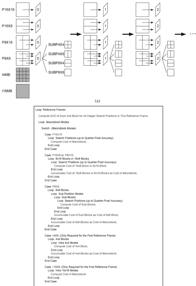
In order to support fast algorithms for multiple reference frames ME, we modified the reference software as follows. Fig. 4(a) and (b) are the illustration and pseudocodes of MB mode decision in our baseline encoder, respectively. Note that now the outer loop is changed to reference frames, and the

Fig. 3. MB mode decision in the reference software baseline encoder. (a) Il-lustration. (b) Pseudocodes.

loop for MB modes becomes inner. At the beginning of each reference frame loop, we compute SADs of each 4 4 block at all search positions only in the current reference frame. At the

end of each reference frame loop, we add a checking procedure to see whether it is all right to skip the remaining reference frames and break the loop. In this way, the computational com-plexity of the prediction part in our baseline encoder is exactly proportional to the number of reference frames searched.

III. STATISTICALANALYSIS

In this section, various statistical analyzes of ten standard se-quences under three different QP values ( and ), which represent high bit rate, medium bit rate, and low bit rate situations, respectively, will be shown.

A. Percentages of Selected Reference Frames

We first analyze the percentages of inter-MBs predicted from different reference frames and intra-MBs. Ref 0 means the MB predicted from the previous frame, and Ref 1 stands for the pre-vious frame of prepre-vious frame, and so on. Note that one MB may be predicted from different reference frames, and we take the farthest reference frame into the statistics. As seen in Table I, 67.58%, 81.35%, and 91.97% of the optimal MVs determined by the full search scheme belong to the nearest reference frame for and , respectively. The possibilities that the optimal MVs fall in other reference frames are much smaller. In other words, in many cases, a lot of computation is wasted on useless reference frames. The result is quite reasonable. In-tuitively, the closer the reference frame is, the higher the cor-relation should be, except for occluded and uncovered objects. Therefore, we should proceed the block matching process from the nearest reference frame to the farthest reference frame. An-other interesting point is that low bit rate cases are more likely to have best reference frames close to the current frame than higher bit rate cases are. This is because the second term of the Lagrangian cost function related to reference frames in-creases with , which results in a larger positive bias on the Lagrangian cost for a larger . That is, at lower bit rates, the effect of becomes much more obvious.

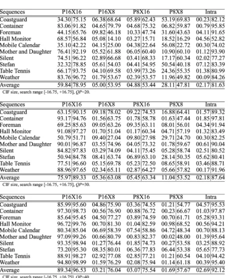
B. Percentages of Selected MB Modes

The result of MB mode decision after intra-prediction and ME from the previous frame is also a very important cue. In Table II, is defined as follows. is the percentage of a selected MB mode after intra-prediction and ME from the previous frame. is the percentage of that the optimal reference frames remain unchanged after five reference frames are searched. We can see that for , there are 59.84%, 05.00%, 04.88%, 28.11%, and 02.17% of the MBs selected as P16X16, P16X8, P8X16, P8X8, and intra, respectively, when only one previous frame is searched. For , there are 75.97%, 05.36%, 05.45%, 11.04%, and 02.18% of the MBs selected as P16X16, P16X8, P8X16, P8X8, and intra, respectively. For , the corresponding percentages are 89.34%, 03.21%, 03.07%, 01.69%, 02.69%. After the re-maining four reference frames are searched, 78.95%, 89.33%, and 96.53% of the 16 16-MBs still remain the same selection for and , respectively. When the block size becomes smaller, such as P16X8, P8X16, and P8X8-MBs, the percentages that the best reference frames do not change tend

TABLE I

STATISTICS OFSELECTEDREFERENCEFRAMES INPERCENTAGES

to be lower. For , it can be seen that

of MBs need only one reference frame, which is quite consistent with the results in Table I. For and 40, the derived percentages are 82.52% and 94.45%, respectively, which are also very consistent with Table I. Additionally, if a MB is split into smaller blocks when only the previous frame is used for ME, it implies that the motion field is discontinuous. In these cases, the MB may cross the object boundaries, where occlusion and uncovering often occur. Thus, there is a greater possibility that the best matched candidates belong to the other four reference frames. Last but not least, it is easier for MBs to split into smaller partitions at higher bit rates. The reason is still related to the Lagrangian cost function. The second term of the Lagrangian cost function related to MB modes increases with , which makes it much more difficult for low bit rate situa-tions to select the partition modes with more side information.

C. Detection of All-Zero Transform Quantized Residues

Now we treat the saving of computation for multiple refer-ence frames in terms of compression. After the prediction pro-cedure, residues are transformed, quantized, and then entropy coded. If we can detect the situation that the transformed and quantized coefficients are very close to zero in the first reference frame, we can turn off the matching process for the remaining

frames since more computation will not further reduce predic-tion errors. This concept is very simple and effective. More-over, discrete cosine transform (DCT), quantization (Q), inverse quantization (IQ), and inverse discrete cosine transform (IDCT) can be also saved by this early detection of all-zero transform quantized coefficients. The quantization steps of 4 4 residues in H.264/AVC are described in the following equations:

(2) (3) (4) (5)

(6) where is the (0–51), is the 4 4 quantized mag-nitude (QM), is the 4 4 transformed residues (TRs),

and is a three-dimensional (3-D)

matrix. If the following inequality (derived from and (6) by setting ) holds:

(7) the QM will be zero, which means each of the 4 4 threshold values becomes a function of and can be implemented as a look-up table. However, TR is not available before transfor-mation. The only information we have after prediction is SAD (SATD or SSD). Thus, we should find the relation between SAD (SATD or SSD) and TR, and then apply the thresholds directly on SAD (SATD or SSD).

The derivation of threshold values is similar to [9]. The dis-tribution of the pixel values after linear prediction in image can be modeled by a Laplacian distribution, which has a signifi-cant peak at zero with exponentially decayed probability at both sides [10]. In addition, the correlation for the pixel values after linear prediction is separable in both horizontal and vertical di-rections. Therefore, we can approximate the input values at the input of transform by a Laplacian distribution with zero mean

and a separable covariance , where and

are the horizontal and vertical distances, respectively, between two pixels, and is the correlation coefficient. Typically, ranges from 0.4 to 0.75, and we use in all our

sim-ulations. Next, let and denote

the4 4 residues at the DCT input and output, respectively. The DCT can be represented in matrix form as follows:

TABLE II

STATISTICS OF SELECTEDMBMODES IN PERCENTAGES

where is the matrix of transform coefficients. The variance of the th DCT coefficients can be written as [11]

(9) where

(10)

and is the th component of the matrix. Since the dis-tribution of has a zero mean, the mean of each will also be zero. The variance of the DCT coefficients will be

(11)

for . In this way, the standard deviation of the DCT coefficients can be estimated by the standard deviation of the pixel values at the DCT input as

(12) Although the generalized Gaussian distribution is the most ac-curate representation of transformed coefficients, for the sake of simplicity, we choose the more commonly used Laplacian dis-tribution to model them [12], [13]. For a zero-mean Laplacian distribution, the probability that a value will fall with ( , ) is about 99%. According to the all-zero situation shown in (7), if

TABLE III VALUES OFTH [QP][i][j]

then the DCT coefficients will be zero after quantization almost all the time. More generally, we can use

(14) where controls the probability of all-zero transform quan-tized coefficients. For , the probability reduces to 94%.

As stated before, is a function of and

. We list some corresponding values of

in Table III. Originally, given a , we can get the 16 values of . In order to detect the all-zero case, we have to compare the 16 values of with different thresholds. However, as shown in (12), is the largest among , which means the probability of a zero dc term after DCT is smaller than that of zero ac terms. Meanwhile, as shown in Table III,

is the smallest among , which

means the quantization step size of dc term is the smallest. Therefore, we only have to compare the dc term in (7) for all-zero detection.

In order to save the extra computation for the standard devia-tion of pixel values at DCT input, we can estimate it from SAD as follows. The expected mean absolute value of a zero-mean Laplacian distributed random variable is

(15) We can approximate the by the SAD of current MB, so we have

(16) If the MB mode is not P16X16, we can still accumulate the SADs of all partitions as SAD of the MB. For example, if the best block mode is P16X8, we can add the SADs of the two 16

8 blocks as the SAD value used in (16). According to (12), (14), and (16), now the all-zero situation holds if SAD is smaller than a predefined threshold, as follows:

(17) Sometimes the user may choose SATD or SSD, instead of SAD, as the criterion of block matching. Now we first derive the relation between SATD and SAD. Once the correlation is found, (17) can be still used for all-zero detection. In the refer-ence software, the SATD of a 4 4 block is defined as half of the sum of absolute values of a two-dimensional (2-D) 4 4 Hadamard-transformed residues.

(18)

(19) For simplicity, we again assume that the residues after Hadamard transform is still Laplacian distributed, so the SATD of a 4 4 block can be approximated by replacing in (9) with

(20) where

(21) From (16), the SAD of a 4 4 block can be approximated as

(22) The relation between SATD and SAD can be seen from (20) and (22). As for the relation between SSD and SAD, it can be deduced by the same probability theory.

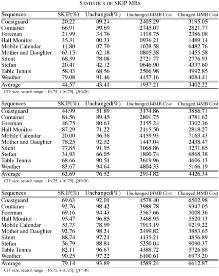
D. SKIP Mode

In H.264/AVC, SKIP mode is a special case of P16X16. Nothing but run of SKIP MBs is transmitted to the decoder. At the decoder side, a SKIP MB is directly reconstructed as a 16

TABLE IV STATISTICS OFSKIP MBS

16 block by prediction from previous one frame with predefined MV (MV predictor in general or zero MV at slice boundary) without any residues. Statistics of SKIP modes are shown in Table IV. The first column is sequence name, the second column is the percentage of MBs selected as SKIP after one reference frame is searched, the third column is the percentage of SKIP MBs that still remain SKIP after five reference frames are searched, the fourth column is the average I4MB cost of the unchanged SKIP MBs (remaining SKIP after five reference frames are searched), and the last column is the average I4MB cost of the changed SKIP MBs (failing to remain SKIP after five reference frames are searched). According to the statistics, for low bit rate cases (high QP), SKIP mode is more favored. The percentages of SKIP MBs after one reference frame is searched are 44.57%, 62.69%, and 79.14% for

and , respectively. Out of these SKIP MBs, 43.41%, 76.52%, and 93.89% still remain SKIP after five reference frames are searched for and , respectively. This is quite reasonable because at low bit rate situations, side information becomes very “expensive.” In addition to values, we found that texture is also a useful information. We use I4MB cost as a rough estimation of texture. Given a value, the higher the

I4MB cost is, the more highly textured the MB is. Based on the statistics, SKIP mode is also preferred in flat areas. The average I4MB cost of the SKIP MBs remaining SKIP after full search among five reference frames is much smaller than that of SKIP MBs changing best modes.

E. MV Inconsistency

Now we try to find the correlation between MVs of variable block sizes and optimal reference frames. After ME from the previous frame, there are one MV for a 16 16 block, two MVs for 16 8 blocks, two MVs for 8 16 blocks, four MVs for 8 8 blocks, and 16 MVs for 4 4 blocks. If the best mode is P16X16, P16X8, P8X16, or P8X8, the definition of MV in-consistency for each of the four MB modes is shown in Fig. 5, respectively. Note that denotes the sum of the L1 distance of the two components between MV1 and MV2. Intuitively, the best MVs of larger blocks and those of smaller blocks should be very similar for objects with homogeneous motion and sufficient texture. For object boundaries where the motion fields are discontinuous, MVs of different block sizes tend to be different. Next, we keep on searching the other four reference frames. If the optimal reference frame of a MB does

Fig. 5. Definition of MV inconsistency of an MB.

not change after five reference frames are searched, we classify these MBs as type I. Otherwise, we classify them as type II. The average MV inconsistency of type I and that of type II for each sequence is shown in Table V. As can be seen, for P16X16, the MV inconsistency of MBs with optimal reference frame be-longing to the farther four frames are much larger than that of MBs predicted by the previous frame. It is easy to apply a clear threshold value on the MV inconsistency for P16X16-MBs after ME from the previous frame is done. If the MV inconsistency is very small, it should be fine to skip the remaining reference frames. For P16X8, P8X16, and P8X8, the MV inconsistency is still a good cue to distinguish between the two categories of MBs, but the threshold value is not that clear. In order not to sacrifice video quality, the threshold values for the MV incon-sistency should not be located in between the average value of type I MBs and that of type II MBs. The threshold should be

biased toward type I to prevent quality loss. Hence, the miss de-tection rate of the best reference frame for type II MBs can be reduced, but the false alarm rate of the best reference frame for type I MBs will be increased.

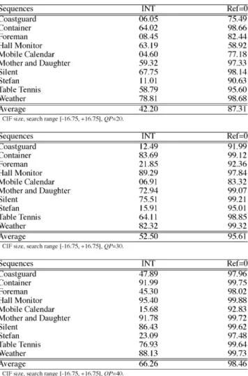
F. MV Location

The above analyses provide useful clues to detect uncovered backgrounds, new objects, or periodic motions for multiple ref-erence frames ME to achieve better coding efficiency without wasting useless computation. In this subsection, we focus on the sampling, which is also one of the reasons why multiple reference frame ME can achieve much better prediction. In the real word, the light field is continuous. On the contrary, the sensor array of camera is discrete. Assume a perfect edge is right across a line of sensor grids. When the object undergoes a

TABLE V

STATISTICS OFAVERAGEMV INCONSISTENCY INUNITS OFQUARTERPIXEL

fractional-pixel motion, the perfect edge will be blurred. Frac-tional-pixel ME can significantly improve the prediction by in-terpolating the subpixels. However, in some cases, especially for highly textured video sequences, fractional-pixel ME is not enough. Multiple reference frames ME provides a better chance for the object to find a matched candidate without the discrete sampling defects. Therefore, we presume that if the MV loca-tion is an integer posiloca-tion instead of a fracloca-tional one, multiple reference frames ME may not be very helpful (unless the MB is an uncovered area or the motion field is not homogeneous). Table VI can somewhat support our claim. After one reference frame ME, if the MVs of a MB are all at integer locations, the probabilities that the optimal reference frame is the previous one frame are 87.31%, 95.61%, and 98.46% for and

, respectively.

IV. SUMMARY ANDPROPOSEDALGORITHM

Before proposing our fast multiple reference frames ME al-gorithm, let us summarize the statistical analyzes as follows.

• Reference frames with smaller temporal distance are more likely to be optimal, especially for the previous frame.

TABLE VI

STATISTICS OFMV LOCATION INPERCENTAGES

• The Lagrangian mode decision is more in favor of closer reference frames at low bit rates than at high bit rates. • The Lagrangian mode decision is more in favor of MB

modes with fewer partitions at low bit rates than at high bit rates.

• If P16X16 mode is selected, the optimal reference frame tends to remain the same.

• If inter-modes with smaller blocks (P16X8, P8X16, and P8X8) are selected, searching more reference frames tends to be helpful.

• For all-zero transform quantized residues, more block matching may be a waste of computation.

• SAD, SATD, or SSD can be used to detect the all-zero case. • If texture is not significant and if the value is large,

SKIP mode is often selected as the best MB mode. • I4MB cost value can be used as a criterion to measure the

complexity of texture.

• If MVs of larger blocks are very similar to those of smaller blocks, it is likely that no occlusion or uncovering occurs in the MB, so one reference frame may be enough. • If MVs of larger blocks are very different from those of

Fig. 6. Rate distortion curves.

the motion field is inhomogeneous, and thus requires more reference frames.

• Sampling the continuous light field by discrete sensor array may blur the sharp edges.

• Fractional-pixel ME can improve the prediction for sam-pling defects, but for highly textured areas, multiple refer-ence frames are more helpful.

• If the object undergoes an integer motion, the prediction gain of multiple reference frames may not be significant. According to the above summary, we propose a fast algorithm for multiple reference frame ME to save the computation of full search and to maintain the same video quality. The flowchart and pseudocodes have already been shown in Fig. 4. In the fol-lowing, we list the steps for each MB to check whether it is necessary to search the next reference frame at the end of each reference frame loop.

• Criterion 1: if ( ), early terminate.

• Criterion 2: if ( && (best )

&& ), early terminate.

• Criterion 3: if (all MV locations integer values), early terminate.

• Criterion 4: if (motion vector inconsistency ), early terminate.

Criterion 1 states that when the best SATD does not exceed , we will stop the searching process. The determination of is described in Section III-C. Note that SATD can be replaced by SAD or SSD.

Criterion 2 is related to SKIP mode. If the best reference frame is previous frame and if the best MV is the same as that of SKIP mode, we call this MB as potential SKIP MB (because be-fore transforming and quantizing the residues, we cannot know for sure if it is really a SKIP MB). For a potential SKIP MB, if its is larger than , the multiple reference frames loop will be early terminated. The determination of is empirically obtained. Recall that SKIP mode is more favored in flat areas and at low bit rate cases, I4MB cost is used to decide

as follows:

if Cost

else if Cost

else Cost (23)

First, if I4MB cost is smaller than 2000, which means the MB is rarely textured, the potential SKIP MB will omit the remaining reference frames. Second, if is larger than 35, the potential SKIP MB will also give up searching the remaining reference frames. Third, ranges from 0 to 35. It is linearly depen-dent of I4MB cost when I4MB cost ranges from 2000 to 8000. The lower the I4MB cost, the smaller the , and the more possible the potential SKIP MB can be early terminated.

Criterion 3 deals with the discrete sampling problem, as de-scribed in Section III-F. If all the MVs of a MB are at integer locations, the block matching process will be finished.

Criterion 4 detects whether the motion field is homogeneous or not. The definition of MV inconsistency can be found in Section III-E. In our experiments, is also empirically obtained. For P16X16 MBs, can be set larger to in-crease the probability of early termination. For other split MBs (P16X8, P8X16, and P8X8), can be set smaller to de-crease the opportunity of early termination.

TABLE VII

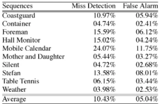
AVERAGEMISSDETECTIONRATE ANDFALSEALARMRATE

V. SIMULATIONRESULTS ANDDISCUSSION

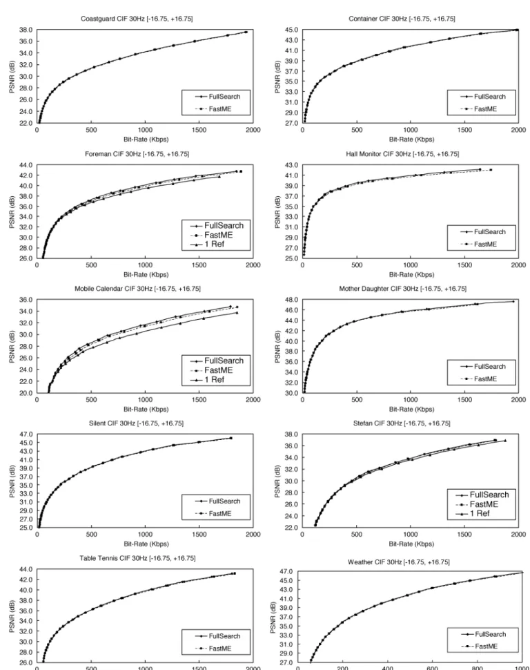
Fig. 6 compares the rate-distortion curves of various stan-dard sequences. For sufficiently textured videos with large and complex motion, the prediction gain of multiple reference frame ME is very significant. Foreman contains an abrupt fast pan of camera, Mobile Calendar has sophisticated texture and zooming camera, and Stefan is a close-up shot of a tennis player running rapidly in the court with many colorful spectators. At medium or high bit rates, the peak signal-to-noise ratio (PSNR) differ-ences between searching five reference frames and searching only one reference frame are about 0.8, 1.2, and 0.4 dB, respec-tively, for Foreman, Mobile Calendar, and Stefan. For other test sequences, searching five reference frames does not provide no-ticeable coding gains, and the rate-distortion curves of searching one reference frame is omitted for clarity. The average PSNR drop of our fast algorithm compared with full search is less than 0.05 dB, so that the full search curve and our fast search curve are hardly distinguishable for each sequence. The degradation of PSNR is only slightly noticeable for Foreman, Hall Monitor, and Mobile Calendar, and is about 0.1–0.2 dB.

Table VII shows the average miss detection rate and the false alarm rate of the optimal reference frames in percentages of MBs. The MVs generated by the full search scheme are used as ground true answers. Miss detection of optimal reference frames terminates the block matching process in the early stage to save computation but runs the risk of video quality degradation. False alarm of optimal reference frames guarantees the same video quality as full search but wastes computation. It is shown that the average miss detection rate is 10.43%, which means about 89.57% of the MBs select the same reference frame as full search. The average false alarm rate is 5.04%, which means 94.96% of the MBs do not require extra unnecessary compu-tation after the best reference frames are found.

Fig. 7 shows the number of average searched frames for the reference software and the proposed algorithm. It is shown that the average number of searched reference frames ranges from 1 to 3.5, which means 30%–80% of ME operations can be saved because the ME operations are in proportion to the number of searched reference frames. We also show the optimal number of searched reference frames, which is defined as

(24)

where , , , , , and denote the

Fig. 8. Comparison with fixed reference frames.

frames 0–4, respectively, by using the reference software. The optimal curves stand for the lower limits of computation that do not suffer any loss of video quality (suppose full search is applied for every reference frame). The gap between the curve of our algorithm and that of the optimal case indicates what we can still improve for more effective reference frame selection. For more motionless sequences, such as Container, Hall Mon-itor, Mother and Daughter, Silent, and Weather, the numbers of searched reference frames are close to the optimal ones. How-ever, for other sequences with higher motion activity, there is still room for further improvement.

Fig. 8 shows the comparison between the rate-distortion performance of our fast algorithm and those of fixed reference frames. Only Foreman, Mobile Calendar, and Stefan are shown here because for other sequences, multiple reference frames cannot contribute to noticeable PSNR gains. Please note that “2 Ref” and “3 Ref” denote 60% and 40% of computation reductions, respectively. The rate-distortion performance of our algorithm is very close to that of “3 Ref” and is better than “2 Ref.” As shown in Fig. 7, our algorithm results in 2.5–3.3 reference frames for the three video sequences. In sum, for cases that multiple reference frames are helpful in compres-sion, “fixed 2 reference frames” provides worse video quality with less complexity, and “fixed 3 reference frames” provides similar video quality with similar complexity. However, for cases that multiple reference frames are useless (low bit rates or other seven sequences), our algorithm can lead to much lower complexity than fixed reference frames. In other words, our algorithm successfully detects when we should or should not search more frames.

Fig. 9 shows the rate-distortion curves and the rate-computa-tion curves for three more test sequences that were not used in the statistics. All the parameters and threshold values are kept the same. Two of the video clips are extracted from the action movies, “Taxi-I” and “Crouching Tiger & Hidden Dragon.” The motion fields of the three test sequences are all very large and complex with moving camera. Simulation results show that our algorithm still performs well in these cases. Most unnecessary calculations of full search scheme are detected. Please note that the optimal number of reference frames for “Taxi-I” is smaller than one because the movie clip has great high motion making the encoder select a lot of intra-MBs.

Now we compare our algorithm with other works. In general, our fast reference frame selection scheme can save a lot of un-necessary ME operations while maintaining the video quality almost identical to full search. Our first idea was published in [14]. It is different from the conventional fast block matching algorithms, such as three-step search [15], one-dimensional full search [16], four-step search [17], diamond search [18]–[20], partial distortion elimination [21], successive elimination [22], and global elimination [23]. The main concepts of conventional methods are decimation of search positions, prediction of MVs, simplification of matching criterion, and early termination of unnecessary SAD calculations. Many researchers [24]–[27] de-veloped their fast algorithms for ME in H.264. Although the concepts are old, the results are quite promising. In [28] and [29], they both proposed the concept of MV composition. MVs of different frames are highly correlated and can be used to pre-dict the MVs for farther reference frames. Fortunately, our al-gorithm and other fast alal-gorithms are orthogonal. The

multi-Fig. 9. Experimental results of other test sequences.

frame ME procedure can combine different algorithms as fol-lows. Given the first reference frame, we can adopt the conven-tional fast search methods. Then, our reference selection criteria can be applied to determine if the remaining frames should be skipped or not. Finally, if it is necessary to keep on searching the next frame, the new concept of MV composition provides a very good solution to further speed up the block matching process for farther reference frames.

VI. CONCLUSION

We proposed a simple and effective fast algorithm for mul-tiple reference frames ME. First, the available information after intra-prediction and ME from the previous reference frame is analyzed. Then, detection of all-zero residues, SKIP mode and complexity of texture, sampling defects, and MV inconsistency are applied to determine if it is necessary to search more frames. Experimental results showed that our method can save 30%–80% of ME computation depending on the sequences while keeping the quality nearly the same as full search scheme. Besides, our scheme can be easily combined with other con-ventional fast algorithms to achieve better performance.

REFERENCES

[1] Draft ITU-T Recommendation and Final Draft International Standard

of Joint Video Specification, ITU-T Rec. H.264 and ISO/IEC 14 496-10

AVC, Joint Video Team, Mar. 2003.

[2] Information Technology—Coding of Audio-Visual Objects—Part 2:

Vi-sual, ISO/IEC 14 496-2, 1999.

[3] Video Coding for Low Bit Rate Communication, ITU-T Rec. H.263, 1998.

[4] Information Technology—Generic Coding of Moving Pictures and

As-sociated Audio Information: Video, ISO/IEC 13 818-2 and ITU-T Rec.

H.262, 1996.

[5] A. Joch, F. Kossentini, H. Schwarz, T. Wiegand, and G. J. Sullivan, “Performance comparison of video coding standards using lagragian coder control,” in Proc. IEEE Int. Conf. Image Process., 2002, pp. 501–504.

[6] Joint Video Team Reference Software JM8.2 May 2004 [Online]. Available: http://bs.hhi.de/~suehring/tml/download/

[7] G. J. Sullivan and T. Wiegand, “Rate-distortion optimization for video compression,” IEEE Signal Process. Mag., vol. 15, no. 6, pp. 74–90, Nov. 1998.

[8] T. Wiegand and B. Girod, “Lagrangian multiplier selection in hybrid video coder control,” in Proc. IEEE Int. Conf. Image Process., 2001, pp. 542–545.

[9] I.-M. Pao and M.-T. Sun, “Modeling DCT coefficients for fast video encoding,” IEEE Trans. Circuits Syst. Video Technol., vol. 9, no. 4, pp. 608–616, Jun. 1999.

[10] N. S. Jayant and P. Noll, Digital Coding of Waveforms. Englewood Cliffs, NJ: Prentice-Hall, 1984.

[11] A. K. Jain, Fundamentals of Digital Image Process.. Englewood Cliffs, NJ: Prentice-Hall, 1989.

[12] J. R. Price and M. Rabbani, “Biased reconstruction for jpeg decoding,”

IEEE Signal Process. Lett., vol. 6, pp. 297–299, Dec. 1999.

[13] R. C. Reininger and J. D. Gibson, “Distributions of two-dimensional DCT coefficients for images,” IEEE Trans. Commun., vol. 31, pp. 835–839, Jun. 1983.

[14] Y.-W. Huang, B.-Y. Hsieh, T.-C. Wang, S.-Y. Chen, S.-Y. Ma, C.-F. Chen, and L.-G. Chen, “Analysis and reduction of reference frames for motion estimation in MPEG-4 AVC/JVT/H.264,” in Proc. IEEE Int.

Conf. Acoustics, Speech, Signal Process., 2003, pp. 145–148.

[15] T. Koga, K. Iinuma, A. Hirano, Y. Iijima, and T. Ishiguro, “Motion compensated interframe coding for video conferencing,” in Proc.

Na-tional Telecommun. Conf., 1981, pp. C9.6.1–C9.6.5.

[16] M.-J. Chen, L.-G. Chen, and T.-D. Chiueh, “One-dimensional full search motion estimation algorithm for video coding,” IEEE Trans.

Circuits Syst. Video Technol., vol. 4, no. 5, pp. 504–509, Oct. 1994.

[17] L.-M. Po and W.-C. Ma, “A novel four-step search algorithm for fast block motion estimation,” IEEE Trans. Circuits Syst. Video Technol., vol. 6, no. 3, pp. 313–317, Jun. 1996.

[18] S. Zhu and K. —. Ma, “A new diamond search algorithm for fast block matching motion estimation,” in Proc. Int. Conf. Inf., Commun. Signal

Process., 1997, pp. 292–296.

[19] J. Y. Tham, S. Ranganath, M. Ranganath, and A. A. Kassim, “A novel unrestricted center-biased diamond search algorithm for block motion estimation,” IEEE Trans. Circuits Syst. Video Technol., vol. 8, no. 4, pp. 369–377, Aug. 1998.

[20] A. M. Tourapis, M. L. Liou, O. C. Au, G. Shen, and I. Ahmad, “Op-timizing the mpeg-4 encoder—advanced diamond zonal search,” in

Proc. IEEE Int. Symp. Circuits Systems, 2000, pp. 647–677.

[21] ITU-T Rec. H.263 Software Implementation. Telenor R&D Digital Video Coding Group, 1995.

[22] W. Li and E. Salari, “Successive elimination algorithm for motion es-timation,” IEEE Trans. Image Process., vol. 4, no. 1, pp. 105–107, Jan. 1995.

[23] Y.-W. Huang, S.-Y. Chien, B.-Y. Hsieh, and L.-G. Chen, “An efficient and low power architecture design for motion estimation using global elimination algorithm,” in Proc. IEEE Int. Conf. Acoust., Speech,

Signal Process., 2002, pp. 3120–3123.

[24] W. I. Choi, B. Jeon, and J. Jeong, “Fast motion estimation with mod-ified diamond search for variable motion block sizes,” in Proc. IEEE

Int. Conf. Image Process., 2003, pp. 371–374.

[25] H. Y. C. Tourapis and A. M. Tourapis, “Fast motion estimation within the H.264 codec,” in Proc. IEEE Int. Conf. Multimedia Expo, 2003, pp. 517–520.

[26] C.-H. Kuo, M. Shen, and C.-C. J. Kuo, “Fast inter-prediction mode decision and motion search for H.264,” in Proc. IEEE Int. Conf.

Mul-timedia Expo, 2004, pp. 663–666.

[27] P. Yang, Y.-W. He, and S.-Q. Yang, “An unisymmetrical-cross multi-resolution motion search algorithm for MPEG-4 AVC/H.264 coding,” in Proc. IEEE Int. Conf. Multimedia Expo, 2004, pp. 531–534. [28] Y. Su and M.-T. Sun, “Fast multiple reference frame motion

estima-tion for H.264,” in Proc. IEEE Int. Conf. Multimedia Expo, 2004, pp. 695–698.

[29] M.-J. Chen, Y.-Y. Chiang, H.-J. Li, and M.-C. Chi, “Efficient multi-frame motion estimation algorithms for MPEG-4 AVC/JVT/H.264,” in

Proc. IEEE Int. Symp. Circuits Syst., 2004, pp. 737–740.

Yu-Wen Huang was born in Kaohsiung, Taiwan, R.O.C., in 1978. He received the B.S. degree in electrical engineering and the Ph. D. degree from the Graduate Institute of Electronics Engineering, National Taiwan University (NTU), Taipei, Taiwan, R.O.C., in 2000 and 2004, respectively.

He joined MediaTek, Inc., Hsinchu, Taiwan, R.O.C., in 2004, where he develops integrated circuits related to video coding systems. His research interests include video segmentation, moving object detection and tracking, intelligent video coding technology, motion estimation, face detection and recognition, H.264/AVC video coding, and associated VLSI architectures.

Bing-Yu Hsieh received the B.S. degree in electrical engineering and the M.S. degree in electronics en-gineering from National Taiwan University, Taipei, Taiwan, R.O.C., in 2001 and 2003, respectively.

He joined MediaTek, Inc., Hsinchu, Taiwan, R.O.C., in 2003, where he develops integrated circuits related to multimedia systems and optical storage devices. His research interests include object tracking, video coding, baseband signal processing, and VLSI design.

Shao-Yi Chien (M’03) was born in Taipei, Taiwan, R.O.C., in 1977. He received the B.S. and Ph.D. de-grees from the Department of Electrical Engineering, National Taiwan University (NTU), Taipei, in 1999 and 2003, respectively.

During 2003 to 2004, he was a Research Staff Member in Quanta Research Institute, Tao Yuan Shien, Taiwan. In 2004, he joined the Graduate Institute of Electronics Engineering, Department of Electrical Engineering, National Taiwan University, as an Assistant Professor. His research interests include video segmentation algorithm, intelligent video coding technology, image processing, computer graphics, and associated VLSI architectures.

Shyh-Yih Ma received the B.S.E.E, M.S.E.E, and Ph.D. degrees from National Taiwan University, Taipei, Taiwan, R.O.C., in 1992, 1994, and 2001, respectively.

He joined Vivotek Inc., Taipei, Taiwan, R.O.C., in 2000, where he developed multimedia communica-tion systems on DSPs. His research interests include video processing algorithm design, algorithm opti-mization for DSP architecture, and embedded system design.

Liang-Gee Chen (S’84–M’86–SM’94–F’01) re-ceived the B.S., M.S., and Ph.D. degrees in electrical engineering from National Cheng Kung University, Tainan, Taiwan, R.O.C., in 1979, 1981, and 1986, respectively.

In 1988, he joined the Department of Electrical Engineering, National Taiwan University, Taipei, Taiwan, R.O.C. During 1993–1994, he was a Visiting Consultant in the DSP Research Department, AT&T Bell Laboratories, Murray Hill, NJ. In 1997, he was a Visiting Scholar in the Department of Electrical Engineering, University of Washington, Seattle. Currently, he is a Professor at National Taiwan University. His current research interests are DSP architecture design, video processor design, and video coding systems.

Dr. Chen has served as an Associate Editor of IEEE TRANSACTIONS ON

CIRCUITS ANDSYSTEMS FORVIDEOTECHNOLOGYsince 1996, as Associate Editor of the IEEE TRANSACTIONS ONVLSI SYSTEMSsince 1999, and as Associate Editor of IEEE TRANSACTIONS ONCIRCUITS ANDSYSTEMSPARTII: EXPRESSBRIEFSsince 2000. He has been the Associate Editor of the Journal

of Circuits, Systems, and Signal Processing since 1999, and a Guest Editor for

the Journal of Video Signal Processing Systems. He is also the Associate Editor of the PROCEEDINGS OF THEIEEE. He was the General Chairman of the 7th VLSI Design/CAD Symposium in 1995 and of the 1999 IEEE Workshop on Signal Processing Systems: Design and Implementation. He is the Past-Chair of Taipei Chapter of IEEE Circuits and Systems (CAS) Society, and is a Member of the IEEE CAS Technical Committee of VLSI Systems and Applications, the Technical Committee of Visual Signal Processing and Communications, and the IEEE Signal Processing Technical Committee of Design and Imple-mentation of SP Systems. He is the Chair-Elect of the IEEE CAS Technical Committee on Multimedia Systems and Applications. During 2001–2002, he served as a Distinguished Lecturer of the IEEE CAS Society. He received Best Paper Awards from the R.O.C. Computer Society in 1990 and 1994. Annually from 1991 to 1999, he received Long-Term (Acer) Paper Awards. In 1992, he received the Best Paper Award of the 1992 Asia-Pacific Conference on Circuits and Systems in the VLSI design track. In 1993, he received the Annual Paper Award of the Chinese Engineers Society. In 1996 and 2000, he received the Outstanding Research Award from the National Science Council, and in 2000, the Dragon Excellence Award from Acer. He is a Member of Phi Tan Phi.