Solving the symmetric tridiagonal eigenvalue problem on hypercubes

Computers Math. Applic. Vol. 25, No. 9, pp. 91-96, 1993 0097-4943/93 $6.00 + 0.00 Printed in Great Britain. All rights reserved Copyright(~) 1993 Pergamon Press Ltd

S O L V I N G T H E S Y M M E T R I C T R I D I A G O N A L E I G E N V A L U E P R O B L E M O N H Y P E R C U B E S

K u o - L I A N G C H U N G

Department of Information Management

National Taiwan Institute of Technology, Taipei, Talwan 10772, R.O.C. W E N - M I N G Y A N

Department of Computer Science and Information Engineering National Taiwan University, Taipei, Talwan 10764, R.O.C.

(Received January 199~; revised and accepted July 199~)

Abstract--Using the methods of bisection and inverse iteration respectively, this paper presents a parallel solver for the calculation of the eigenvalues of a real symmetric tridiagonal matrix on hypercube networks in O(ml logn) time using O(n2/logn) processors, where ml is the number of iterations. The corresponding eigenvectors problem can be solved in O(log n) time on the same networks.

1. I N T R O D U C T I O N

Given a real s y m m e t r i c tridiagonal m a t r i x of order n - 1, A = (bi_laibi) for 1 < i < n - 1. Let Aj be the leading j x j principal s u b m a t r i x of A and define the characteristic polynomial Qj(A) = det(Aj - AI), 1 < j < n - 1. We assume t h a t no off-diagonal element is zero, i.e., bi ~ 0 for all i, 1 < i < n - 2. T h e original problem, namely, solving the s y m m e t r i c tridiagonal eigenvalues and eigenvectors problem, can be divided into two subproblems if some bi is equal to zero. By simple d e t e r m i n a n t a l expansion [1], the S t u r m sequence is derived by

Qj(A) = (aj - A)Qj_I(A) - b2_IQj_2(A)

(1)

with the initial conditions Q0(A) = 1 and QI(A) = al - A.

Based on modified S t u r m sequence evaluations coupled with the inverse iteration [2,3], where (1) is rescaled and replaced by the nonlinear recurrence: PI(A) -- al - A , Pi = a i - A - (b~_l)/(Pi_l) , Ipsen and Jessup [4] proposed a parallel algorithm consisting of six compli- cated p a r t s to solve the eigenvalues and eigenvectors problems on a p-processor hypercube. In their algorithm, each processor in the h y p e r c u b e network c o m p u t e s k ( = n / p ) eigenvalues and k eigenvectors of A. W i t h o u t the time-complexity analysis, they presented the numerical results and timings for Intel's iPSC-1. Evans and Margaritis [5] proposed a pipelining systolic array to find all the eigenvalues in O ( m n ) time using O ( n ) processors, where m is the n u m b e r of iterations. In addition, by utilizing the LU decomposition m e t h o d with partial pivoting, the corresponding eigenvectors can be solved in O(n 2) time using O(1) processors.

By using the m e t h o d s of bisection and inverse iteration respectively, this p a p e r presents a parallel solver for the calculation of the eigenvalues of a real s y m m e t r i c tridiagonal m a t r i x on h y p e r c u b e networks in O(rnl log n) time using e ( n ~ / l o g n) processors, where m l is the n u m b e r of iterations. T h e corresponding eigenvectors p r o b l e m can be solved in O ( l o g n ) t i m e on the s a m e networks. Under the s a m e cost, theoretically, our solver is faster t h a n the one by Evans and Margaritis.

This research is supported by the National Science Council of the Republic of China under contract NSC80-0415- E011-10. We are indebted to the reviewers for making some valuable suggestions and corrections that lead to the

improved version of the paper.

Typeset by .AA4~TF~ 91

92 K.-L. CSUNG, W.-M. YAN

2. T H E C O M P U T A T I O N O F T H E E I G E N V A L U E S

To use the Givens' bisection method for finding all the eigenvalues, we first require the following theorem.

THEOREM 2.1.

[1] The number of eigenvalues smaller than a given z

is

equal to the number

o f

sign disagreements, S(z), in the Sturm sequence Qo(x), Q1 (x),..., Q,_ 1 (x).

In order t h a t the above theorem should be meaningful for all values of x, we must associate a sign with zero values of

Qi(z).

If

Qi(x)

= 0, then

Qi(x)

is taken to have the same sign to t h a t of

Q,_l(X).

It is easily proved that no two consecutive terms

Qi-l(x)

and

Q,(x) are

zero [3].

For finding the feasible interval, say, (a0,/30), to confine every eigenvalue of A, we need the following theorem due to Gerschgorin [3].

THEOREM 2.2.

Every eigenvalue

o f

A lies in the interval (no, #o), where ao =

rain (ai -

x<_i<,-1

Ibi-xl-

Ibil)

and/30 = max

_L<i<,-I

(ai "4"

[bi-ll + Ib/I).

Let A~(A) denote the i th largest eigenvalue of A. From Theorem 2.2, we know that any A~(A) must lie in the interval (ao,/30). First, let cl = (ao +/3o)/2 be the middle point of (ao,/3o). Then compute the sequence Q o ( c l ) , Q x ( c l ) , . . . , Q , - l ( c , ) and hence

determine S(m). If

s ( m ) <

i,

then set (~1 = c1 and/31 =/30; otherwise set a l = a0 and/31 = cl. Next, let cx = ( a l +/31)/2, and we repeat the above bisection process again. Finally, we can locate Ai(A) in an interval

(am,, bin,)

of width (rio -

no)~2 m~

after mx iterations. Totally, there are n - 1 such eigensystems to be solved.

For each task to compute Ai(A), observe that the major work in each iteration is to first compute the prefix values of

Q , - , ( c l ) ,

and then to determine the sign disagreement

S(c~).

Using the recursive-doubling method [6], the Sturm sequence (1) can be rewritten as

t c

Qj(cl) = Uj(cl)Q~_,( ,),

where Q~ (cl) = (Qj (cx), Qj-1 (cx))t with Q~ = (1,0)* and Mj (cl) = (v, w), where v = (aj - c x , 1)*,

I b 2 0~' = Q ' - l ( m ) ,

w = ~ - j - l , ] and b0 0. After finishing the prefix computation of each Qi(Cl) can be determined directly when we select the first component of Q~(cl).

An overlaid tree network to perform the typical prefix computation has been presented in [7]. Given Q~, Ml(Cx), M2 ( C l ) , . . . ,

M7(cl),

an example of how the overlaid tree network works for the prefix computation of

Q7(cl)

is shown in Figure 1.

stage 0 stag," 1 stag(: 2 ~tagc ,~ ~lage 4

~ o " ~ \ "O----'K~ " Q O ~C') M~ (c,)----~O.~ . . . ~ \ : . . , \- k~"~4~--.C) -Q--- O ~ (c:)

M T ( C , ) * O - ~ - " Q ~ . . . . ' . j - - ~ 0 7 ( C , )

step 1 step 2 step 3 stcp 4

F i g u r e 1. A n e t w o r k for c o m p u t i n g t h e prefix v a l u e s o f Q l ( C l ).

In Figure 1, the white nodes in the leftmost stage 0 are used for preparing input d a t a only. The white nodes in stages 1, 2, and 3 are used for transmitting d a t a only. The black nodes perform the 2 x 2 matrix multiplications. The slash nodes ® select the desired data. Initially, 8 input d a t a

Q'o, Mx(c,), M2(cl),..., M~(cl)

are fed into the white nodes in stage 0. Passing through five stages, the prefix values of

Q7(cl)

are obtained. For exposition, let the number of input d a t a Q~,

Ml(cl), M2(cl),..., M , - , ( c l )

be a power of 2, i.e., n = 2 r. Therefore, there are log n + 2 stages in this network, and the computation time is only O(log n) time. If each node is implemented by a processor, the number of processors is as large as O(n log n), which is reduced to

O(n/log

n) in Section 3, while retaining the same time complexity.

Symmetric tridiagonal eigenvalue problem 93 3. M A P P I N G I N T O T H E H Y P E R C U B E N E T W O R K

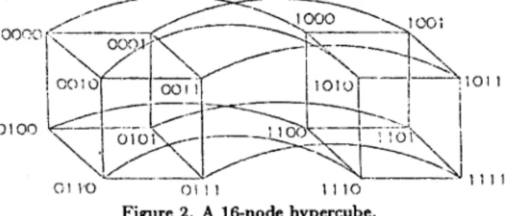
We now present how to map the prefix computations introduced in Section 2 into a hypercube network. An r-dimensional hypercnbe [8] has n = 2 r nodes. Each node is incident to r ( = log n) other nodes, one across each dimension. T h e node can be labeled from 0 to 2 r - 1 (in binary- reflected Gray code, which will be defined later), and two processors are linked if and only if their labels differ in exactly one bit position. Figure 2 shows the construction of a 16-node hypercube from two 8-node hypercubes.

/ - I

i / / / 1 / ! I

"-..l.J

O1 t ' 0 C) l ] 1 1 1 1 0 Figure 2. A 16-node hypercube.

Refer to Figure 1 again. Denote the i th processor of stage k by P ( i , k ) , 0 < i < n - 1,

1 < k < l o g n . At step k (from stage k - 1 to stage k), 1 < k < logn, processor P ( i , k - 1) sends

its d a t a to processors P(i, k) and P ( j , k), where j = i + 2 k-1. Processor P ( j , k) receives the d a t a

sent from P ( j - 2 k - i , k - 1) and calculates it with the d a t a sent from P ( j , k - 1).

Let Gi = g l o g n - l g l o g n - 2 . . . g o be the binary-reflected Gray code of i = bios,~-lbtogn-2.., bo,

i.e.,

~logn--1 : b | o g n - l ,

g j = b j + l ~ b j f o r 0 < j < l o g n - 2 ,

where ~ is the exclusive-or operator [9]. We denote the i th processor by Gi (simply called

processor Gi) and will simulate all the functions of P ( i , k ) , 1 <_ k <_ logn, on that processor.

By [10], we have the following lemma and theorem.

L E M M A 3.1. The binary-reflected Gray codes Gi and Gi+2k-1, k > 1, differ in precisely two bit positions. Those bits are gt and g,, where s is the bit position in which the carry stops propagating when 2 k- 1 is added to i.

THEOREM 3.2. In simulating the overlaid tree network on the n-node hypercube network, two data transfer steps in the hypercube are needed for each step in the overlaid tree network except the first, which needs only one data transfer step. Let the edge in the hypercube be bidirectional. The following routing guarantees disjoint data transfer paths: processor Gi sends data to pro- cessor x with the address obtained by complementing the lower order bit where Gi and Gi+9.k-i differ, then processor x sends its data to processor Gi+2k-~.

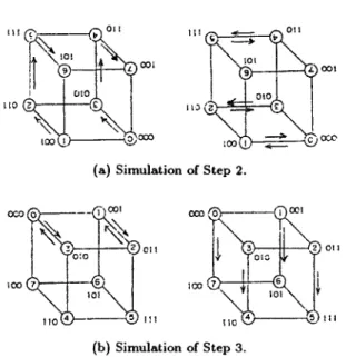
T h e simulations of Step 2 and Step 3 of Figure 1 on an 8-node cube are illustrated in Figure 3a and 3b respectively. For processor P(i, 1) of Figure 1, the corresponding processor in the 8-node

cube as shown in Figure 3 is denoted by the index i, which is encapsulated in a circle, and is associated with Gi. First, the d a t a in processor Gi, 0 < i < 5, are transmitted to the intermediate

processor x simultaneously. T h e direction of each d a t a transfer is denoted by the arrow as the left figure of Figure 3a shows. Next, the d a t a in processor z are t r a n s m i t t e d to processor Gi+2 as the right figure of Figure 3a shows, and then the 2 x 2 matrix multiplications are performed in parallel. For simplicity, throughout the rest of the paper, we assume t h a t the cost of one d a t a transfer is equal to the cost of one computation. This assumption is reasonable since the ratio of one d a t a transfer cost and one computation cost can be bounded by a constant factor [11]. This assumption will not alter the result of complexity analysis when we use the big O notation. As a result, Step 2 of Figure 1 can be simulated by two steps on the 8-node cube. By the same way, Step 3 of Figure 1 can be simulated by two steps as shown in Figure 3b. In general, the prefix values of Q n - l ( C l ) can be computed in O ( l o g n ) steps on a hypercube of n nodes. Note

t h a t the tree-like computations of Figure 1 can also be m a p p e d onto an Omega network [12], and

94 K.-L. CHUNG, W.-M. YAN

~

oo~ ~ o o l

rIO 1~3(

. ~ l ~ t ) ~,,,,x~,~ 000 ~O'J ~ o¢..o (a) Simulation of Step 2.

(b) Simulation

_ _ 001

~

011

of Step 3.

Figure 3. Simulation of Figure 1 on an 8-node hypercube.

if the adjacent pairs of nodes in an Omega network correspond to pairs of nodes along different dimensions of a hypercube, then the above mapping between trees and hypercubes become clear. Suppose we have t processors, t <_ n. Let the n input data

(Q'o,Ml(Cl),...,M,_l(Cl))

be evenly divided into t pipes to be stored in the processors separately. Algorithm 3.1 describes how the hypercube network works.

ALGORITHM 3.1.

PHASE 1. (Local computations)

Each processor Gi sequentially computes

nit

prefix values from its corresponding pipe of

n/t

data and stores them in its local memory. The register

R(Gi)

residing in processor

Gi

contains the result

M(i+l),/t-l(Cl) x ... x Min/t(Cl) ,

0 < i < t - 1, where M0(cl) = Q~.

PHASE 2. (Global prefix computations)

All the processors work together using the routing mechanism described in Theorem 3.2 for prefix computations on the content of

R(Gi)'s.

The register

R(Gi)

holds the value Q~i+ 1)n/t-1 (Cl), 0 < i < t - 1 .

PHASE 3. (Adaptation)

Each processor Gi except processor G0 receives the value of

R(GI-1)

from processor Gi-1, and sequentially modifies the prefix values calculated in Phase 1 by multiplying the value of R(Gi-1) to each of those local prefix values.

Both Phase 1 and Phase 3 contain

O(n/t)

computation steps. Phase 2 contains 2 1 o g t - 1 data transfer steps and O(log t) computation steps. By the assumption of one data transfer cost being equal to one computation cost, the three-phase algorithm takes

O(n/t +

log t) time to finish

I C

computing all the prefix values of Q , - I ( 1 ) . It needs O(1) time to obtain the prefix values of

qn--l(C1).

We use n = 8 and t = 4 as an example to illustrate the algorithm briefly. Initially, the 8 input data

(Mo(cl),

M l ( c l ) , . . . , MT(cl)) are evenly divided into 4 pipes, each containing 2 data. The processor Gi, 0 < i < 3, has the data M2i(Cl) and

M2i+l(Cl).

After Phase 1 of Algorithm 3.1, the register

R(Go)

has the resultant of Ml(Cl) x

Mo(cl), R(G1)

has the resultant of

M3(cl)

x M~(Cl), and so on. After Phase 2,

R(Go)

has the resultant of Ml(Cl) x M0(cx),

R(G1)

has the resultant of M3(cl) x ... x

Mo(cl),

and so on. After Phase 3 for adaptation, the prefix values of Q~.(Cl) are obtained, and then the prefix values of Qt(cl) are obtained directly. That is, processor Go has the values {Q0(cl), Ql(cl)}, G1 has the values {Q2(Cl), Q3(Cl)}, and so on.

For the subsequent parts of computation, namely, computing the number of sign disagreements,

S(cl),

the similar three-phase concept works equally well. In Phase 1, each processor Gi does sum up the number, say

Si(cl),

of its corresponding pipe of sign disagreement sequentially. This step

Synunetric tridiagonal eigenvalue problem 95 needs about O(n/t) computation steps. In Phase 2, processor Gi sends the value of Q(i+l)nl,-I to processor Gi+l for 0 < i < t - 2 , and the value of Sj(Cl), 1 < j < t - 1, is updated based on the sign disagreement of Qjn/t-1 and Qjn/t. In Phase 3, these new values of Si(Cl)'S, 0 < i < t - 1 are summed by a tree method. It takes about O(logt) steps because it is well known t h a t a tree-structured computation can be performed in logrithmic time on a hypercube network. We have the following lemma.

LEMMA 3.3. The number o f sign disagreements,

S(c1),

in the Sturm sequence of (1) can be determined in O(n/t + logt) time on a hypercube network o f t processors.

The performance of a parallel algorithm can be measured by Cost = Number of Processors x Execution Time. Given a problem, if the cost of a parallel algorithm matches the sequential time lower bound within a constant, the parallel algorithm is said to be cost-optimal. In the case of determining the sign disagreement in the Sturm sequence, since there are n - 1 signs to be produced and calculated, the sequential time lower bound is f~(n). For the bootstrapping method [13], if we set t = O(n/logn) in Lemma

3.3,

we have the following theorem.

THEOREM 3.4. The value o f S(cl) can be cost-optimally determined in O(logn) time on a hypercabe network of O(n/ log n) processors.

Now let's return to the eigenvalues problem. From Theorem 3.4, one can see t h a t a sign disagreement can be determined in O(log n) time on a log(n/log n)-dimensional hypercube. To solve n - 1 sign disagreements simultaneously, we need n - 1 such hypercubes. A natural approach is to connect these n - 1 hypercubes, each of them an n~ log n-node hypercube, by a simple network. Therefore, we have the following main result.

THEOREM 3.5. The eigenvalues problem can be solved in O(ml log n) time on hypercube net- works o f O ( n 2 / l o g n) processors, where ml has been discussed in Section 2.

4. T H E C A L C U L A T I O N O F T H E E I G E N V E C T O R S

Using the inverse iteration method [2,3], the eigenvector x of A with respect to the eigenvalue can be approximated by solving the symmetric tridiagonal system

(A - M ) x = b, (2)

where b is an arbitrarily normalized vector.

If we apply the cost-optimal parallel tridiagonal system solver [14], then (2) can be solved by means of Gaussian elimination and backward substitution. The first iterate of the eigenvector x, the approximated eigenvector x l can be determined in O(logn) time on a hypercube using O(n/log n) processors. Next we solve the system

( A - A I ) x 2 = x l

again, and the improved approximated eigenvector xa is obtained.

In practice, if we select a suitable b, then the second vector xa would usually be a very good approximation to the exact eigenvector corresponding to the specific eigenvalue ,L How to determine the choice of initial vector b is suggested in [3].

For each eigenvalue Ai, 1 _< i _< n - 1, the corresponding approximated eigenvector can be determined in O(logn) time on a log(n/logn)-dimensional hypercube. To solve n - 1 such symmetric tridiagonal systems simultaneously, we need n - 1 such hypercubes. By the same arguments in Section 3, we have the following theorem.

THEOREM 4.1. The eigenvectors problem can be solved in O(log n) time on hypercube networks Ol e O ( n 2 / l o g n) processors.

96 K.-L. CHUNG, W.-M. YAN

5. C O N C L U D I N G R E M A R K S

A parallel algorithm for solving the symmetric tridiagonal eigenvalues and eigenvectors problem has been presented. O n hypercube networks of O(n2/log n) processors, the eigenvalues problem can be solved in O ( m l log n) time; the corresponding eigenvectors problem can be solved in O(log n) time.

Under the same cost, theoretically, our parallel solver is faster than the one proposed by Evans and Margaritis [5]. However, our parallel solver m a y suffer from the possibility of overflow and underflow in the absence of rescaling before each iteration. In practice, if the floating-point number system has high precision, the drawback can be remedied.

REFERENCES

1. J.W. Givens, A method of computing eigenvalues and eigenvectors suggested by classical resttlts on symmetric matrices, U.S. Nat. Bur. Standards Applied Mathematics Series 29,117-122 (1953).

2. W. Barth, R.S. Martin and J.H. Wilkinson, Calculation of the eigenvalues of a symmetric tridiagonal matrix by the method of bisection, Numer. Math. 9,386--393 (1967).

3. J.H. Wilkinson, The Algebraic Eigcnvalue Problem, Clarendon Press, Oxford, (1965).

4. I.C.F. Ipsen and E.R. Jessup, Solving the symmetric tricliagonal eigenvalue problem on the hype~cube,

S I A M J. Sei. Stat. Comput. 11 (2), 203-229 (1990).

5. D.J. Evans and K. Margaritis, Systolic designs for the calculation of the eigenvalues and eigenvectors of a symmetric tricliagonal matrix, Inter. J. Computer Math. 33, 1-12 (1990).

6. H.S. Stone, An efficient parallel algorithm for the solution of a tridiagonal linear system of equations, J. A CM 20 (1), 27-38 (1973).

7. H.S. Stone, Introduction to Computer Architecture, Science Research, Chicago, IL, (1980). 8. C.L. Seitz, The cosmic cube, Comm. A C M 2 8 (1), 22-33 (1985).

9. E.M. Reigold, J. Nievergelt and N. Deo, Combinatorial Algorithms: Theory and Practice, Prentice-Hall, Englewood Cliffs, N J, (1977).

10. S.L. Johnson, Solving tridiagonal systems on ensemble architecture, SIAM J. Sci. Stat. Comput. 8 (3), 354-392 (1987).

11. Y. Saad and M.H. Schultz, Data communication in hypercubes, J. of Parallel and Distributed Computing 6,115-135 (1989).

12. H.S. Stone, Parallel processing with the perfect shuffle, IEEE Trans. on Computers C-20 (2), 153-161 (1971).

13. D.H. Greene a n d D.E. Knuth, Mathematics for the Analysis of Algorithms, 2 nd ed., BirkhKuser, Boston, (1982).

14. F.C. Lin and K.L. Chung, A cost-optimal parallel tridiagonal system solver, Parallel Computing 15,189-199