EMIA: A new efficient algorithm for indirect associations mining

EMIA: A New Efficient Algorithm for Indirect Associations Mining

Wen-Yang Lin

Dept. of Comp. Sci. & Info. Eng. National University of Kaohsiung

Yi-Ching Chen

email: [email protected] email: [email protected]

Abstract—Indirect association is a new type of infrequent pattern, which is to “indirectly” connect two rarely co-occurred items via a frequent itemset called mediator, and if appropriately utilized it can help to identify real interesting “infrequent itempairs” from databases. In this paper, we propose a new efficient algorithm, namely EMIA, for mining indirect associations. The proposed EMIA algorithm improves the deficiency of the leading algorithm HI-mine*, alleviating unnecessary data transforming processes, thus can generate all indirect associations more efficiently using less memory storage. Experiments on both synthetic and real datasets are also made to show the effectiveness of the proposed approaches.

Keywords-Data mining, infrequent pattern; indirect association; mediator

I. INTRODUCTION

Indirect association, proposed by Tan et al. [10], is a new type of infrequent pattern [4, 8, 16], which provides a new way for interpreting the value of infrequent patterns and can effectively reduce the number of uninteresting infrequent patterns. The concept of indirect association is to indirectly connect two rarely co-occurred items via a frequent itemset called “mediator”, and if appropriately utilized it can help to identify real interesting “infrequent itempairs” from databases. A formal definition of indirect associations is described below.

Definition 1 An indirect association 〈x, y | M〉 means that an itempair {x, y} is indirectly associated via a mediator M if it satisfies the following three conditions:

1. Itempair support condition: sup({x, y}) < σs;

2. Mediator support condition: sup({x} ∪ M) ≥ σf and sup({y} ∪ M) ≥ σf;

3. Mediator dependence condition: dep({x}, M) ≥ σd and dep({y}, M) ≥ σd,

where σs, σf and σd are itempair support threshold, mediator support threshold and mediator dependence threshold, respectively. dep(R, S) is a measure of the dependence between itemsets R and S. The well-known dependence function IS measure IS(R, S) (= P(R, S) / sqrt(P(R) × P(S))) is used in this paper.

For example, we know that Coca-cola and Pepsi are competitive products and could be replaced each other. So it is very likely that there is an indirect association rule that consumers usually buy a kind of cookie tend to buy together

with either Coca-cola or Pepsi but not both 〈Coca-cola, Pepsi | cookie〉. Suppose that the Coca-Cola Company wants to increase the sales of cola and also attempts to attract consumers who originally want to buy Pepsi. For this purpose, they can promote the bundling package that includes their cola and the cookie. Many approaches have been proposed and applied on different fields, including e-commerce, text mining, bioinformatics, etc. [6, 7, 11, 12].

The original indirect association mining approach proposed by Tan et al. [10], called INDIRECT, consists of two phases, frequent itemsets mining and indirect associations mining phases. Any frequent itemsets mining approaches can be used in phase 1. The derived frequent itemsets are then used to generate indirect association patterns. However, it is time-consuming to generate all frequent itemsets before mining indirect association.

In this paper, we propose a new efficient algorithm, namely EMIA, for mining indirect associations. The proposed EMIA algorithm improves the deficiency of the leading algorithm HI-mine* [16], alleviating unnecessary data transforming processes, thus can generate all indirect associations more efficiently using less memory storage. Experiments on both synthetic and real datasets are also made to show the effectiveness of the proposed approaches.

II. RELATED WORK

Existing researches on indirect association mining can be divided into two categories, either focusing on proposing more efficient mining algorithms [3, 13, 14, 16] or extending the definition of indirect association for different applications [3, 6, 7].

Wan and An [13, 14] proposed an approach, called HI-mine, for improving the efficiency of the INDIRECT algorithm. Rather than generating all frequent itemsets, HI-mine focuses on finding all itempairs first, and then pursues the mediator of each itempair. The HI-mine algorithm adopts a data structure based on the concept of dynamic transaction projection of frequent item, through which there is no need for doing any join operation for candidate generation. Instead, Hi-mine generates two new sets, indirect itempair set (IIS) and mediator support set (MSS), by recursively building the HI-struct for the database. Then indirect associations are discovered from these two sets directly.

Chen et al. [3] also proposed an indirect association mining approach that was similar to HI-mine, namely MG-Growth. The differences between them are that the directed graph and bitmap are used in MG-Growth for constructing the indirect itempair set. The corresponding mediator graphs are then generated for deriving indirect associations.

As to extending the definition of indirect association, Kazienko et al. applied indirect association on web pages recommendation system [6, 7]. Chen et al. [3] proposed an approach for mining indirect association of items by adding time feature of goods. Since each item has its lifespan, the relationships of new coming items can thus easily be discovered.

A. Review of Hi-mine*

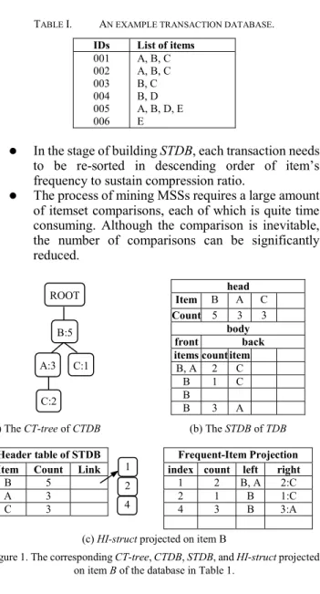
The HI-mine* algorithm [16] also proposed by Wan and An, is an enhancement of the HI-mine algorithm. HI-mine* adopts a more compact data structure call Super Compact Transaction Database (STDB), on which some optimization strategies are introduced, including only one database scanning, direct frequent item projecting, and dynamic infrequent item pruning. The STDB is a compressed transactions data that hopefully can be stored into memory. Any transactions that differ only in the last item are combined into a new transaction in STDB, in the form of composed of two parts, head and body. However, different from CTDB, the body is further divided into two parts, front and back, where the front stores the prefix items of the compressed transactions except the last items, which along with their counts are stored in the back part.

The HI-mine* algorithm consists of three phases. In the first phase, it transforms the original transaction database into an STDB through four intermediate steps, transferring the transaction database into the CT-tree, next, transferring CT-tree into the CTDB (Compact transaction Database), then transferring CTDB into another CT-tree, and finally transferring CT-tree to STDB. In the second phase, it builds an HI-struct from a STDB and then dynamically adjusts and mines the HI-struct to compute the IIS and MSSs. The HI-struct consists of a header table of STB, storing the frequent items and the links pointing to the transactions in STDB where it appears, and a dynamic changing table storing the resulting projection of STDB on that item. In the third phase, the complete set of indirect associations is generated from IIS and MSSs. Fig. 1 illustrates the corresponding CT-tree, CTDB, STDB, and HI-struct projected on item B of the transaction database in Table 1 with σf = 0.5.

B. Problem of Hi-mine*

In the study of HI-mine* we observed some shortcomings:

z The construction of STDB requires many data

conversion steps, and the cost for data conversion is proportional to the transaction length, i.e., the longer the transaction length is, the more time the conversion will require.

TABLE I. AN EXAMPLE TRANSACTION DATABASE. IDs List of items

001 002 003 004 005 006 A, B, C A, B, C B, C B, D A, B, D, E E

z In the stage of building STDB, each transaction needs

to be re-sorted in descending order of item’s frequency to sustain compression ratio.

z The process of mining MSSs requires a large amount

of itemset comparisons, each of which is quite time consuming. Although the comparison is inevitable, the number of comparisons can be significantly reduced. head Item B A C Count 5 3 3 body front back items count item

B, A 2 C

B 1 C B B 3 A (a) The CT-tree of CTDB (b) The STDB of TDB

Header table of STDB Item Count Link

B 5 A 3 C 3

Frequent-Item Projection index count left right

1 2 B, A 2:C

2 1 B 1:C 4 3 B 3:A (c) HI-struct projected on item B

Figure 1. The corresponding CT-tree, CTDB, STDB, and HI-struct projected on item B of the database in Table 1.

III. ALGORITHM EMIA A. Basic Concepts

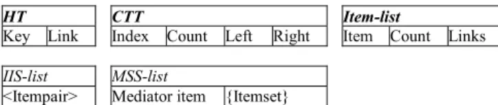
Our proposed approach, the EMIA (Efficient Mining of Indirect Association) adapts the data compression concept used in HI-mine* but using more efficient way to achieve the same purpose. The data structures used in the EMIA algorithm include (shown in Fig. 2)

z CTT: The CTT (Compact Transactions Table) is used for merging identical transactions and combining analogical transactions. It has four parts: firstly, the left part that contains the same set of items, secondly, the right part that contains the list of all different items with their count values, thirdly, the counting sum of all item’s count value which contains in right part, and last, the index as an unique value for identification.

z HT (Hash Table): It is used to store the hashed value

of the left part of the transaction and links as pointers to the related row in the CTT.

1 2 ROOT C:1 C:2 A:3 B:5 4

z Item-list: It is used for keeping all items and its

frequency and link to the corresponding row in CTT.

z MSS-list: It is used for storing candidate mediators. z IIS-list: It is used for indirect itempair sets.

HT CTT Item-list

Key Link Index Count Left Right Item Count Links

IIS-list MSS-list <Itempair> Mediator item {Itemset}

Figure 2. The data structures used in the EMIA algorithm.

With the new data structures, later we will show that our algorithm can overcome all of the aforementioned shortcomings of Hi-mine*.

z We do not use the item frequency to re-sort

transaction but instead sorting items in alphabetical order.

z We no longer need CT-tree, CTDB and STDB

through these four stages to generate the Frequent-Item Projection Table. Instead, we used HT to help us quickly identify whether the left part is already existed. If found, we can quickly update the data in the CTT.

z In the building of CTT stage, we add the pointer link of the CTT to another new structure, namely Item-list, for reducing the number of comparisons.

B. Algorithm Details

The EMIA algorithm consists of three main phases: Compact transactions table construction, MSSs and IIS construction and indirect association generation. In what follows, we describe the process of each phase.

In the Transaction Projection phase, each transaction is split to two parts, left and right; the right corresponds to the last element of the transaction and left stores the other elements, i.e., a transaction t = {x1, x2, ..., xm} is divided into left = {x1, x2, ..., xm-1} and right = {xm}. Next, we search in CTT to see if there is any transaction with the same left part as t. To speed up the searching process, we adopt the hash technique and store the index pointing to the corresponding row in CTT in the HT table, with key storing the left part of t and link storing the index. In this way, we insert the left part and right part of t into CCT, if the searching result is negative; otherwise, we update the corresponding count field in CCT, which denotes the number of transactions having the same left part, and the count of the item stored in the right field. In the same time, each item in transaction t along with the index in CCT is also inserted into the Item-list if it is a new observed item or its count is updated, otherwise.

After each transaction in D is transformed and inserted into the CTT, we remove infrequent items from CTT and Item-list. This is because we only need those frequent items to construct MSSs and IIS; removing the infrequent items can further improve the performance.

The core phase, MSSs and IIS construction is responsible for generating candidate MSSs and IIS by using a divide-and-conquer strategy. Specifically, our approach can be considered as a mediator-oriented searching process,

which follows the prefix set-enumeration framework [9]. For example, assume the Item-list contains {A, B, C, D} frequent items. We first generate A as a candidate mediator, forming subsets of CTT containing any left or right fields that A appears. Then inspect all other items in Item-list to see if each of them, can be combined with A. For example, for item B, we check if sup(A, B) ≥ σf and dep(A, B) ≥ σd . If so, we add A into the mediator set of B, i.e., MSS(B). The above process continues in the order of AB, AC, AD, then ABC, ABD, and back to B, BC, BC, etc.

In order to find IIS and MSSs that contain itemset {a1, a2} a subset S12 is created. In S12, we calculate the support of itemset {a1, a2} and check if the support is greater than or equal to σf and whether the dependency of {a1, a2} is greater than σd. If so, then a1 and a2 arecandidate mediators and we add a2 to MSS(a1) and add a1 to MSS(a2). Secondly, we partition S12 into smaller subsets S123, S124, ..., S12n for finding other mediators until there is no subset with support greater than σf. On the other hand, if the support of {a1, a2} is less than σs, then itemset {a1, a2} is a candidate IIS and so is added to the IIS-list.

In the indirect association generation phase, we use each candidate IIS in IIS-list to find mediators. For any two IIS {a1, a2} in the IIS-list, we only have to check if they have the same mediators in MMS(a1) and MSS(a2). For each common mediator M in MMS(a1) ∩ MSS(a2), we obtain an indirect association 〈a1, a2 | M〉.

C. An Example

In this section, we will illustrate the EMIA algorithm using the example in Table 1. Suppose σs = σf = σd = 0.5, where σs, σf and σd are itempair support threshold, mediator support threshold and mediator dependence threshold, respectively.

1) Transaction Projection Phase: In this phase, we project each transaction to three data structures: HT, CTT and Item-list. The first transaction is {A, B, C}. Below are the steps for projecting this transaction. (1) The transaction is split into left={A, B} and right={C} and added into CTT. (2) Add key {A, B} and the pointer 1 to HT. (3) Add each item in this transaction and the corresponding pointer link in CTT to Item-list. Fig. 3 shows the result after processing the first transaction.

HT CTT Item-list

Key Link Index Count Left Right Item Count Links A, B 1 1 1 A, B C:1 A B C 1 1 1 1 1 1 Figure 3. The resulting structures after processing the first transaction.

The second transaction is the same as the first one, so we only have to update the count in CTT and Item-list. Next, we process the third transaction. Since the left part B is not found, so a new tuple is created in HT and CTT to accommodate this transaction. The process continues till only one item is contained, i.e., the sixth transaction. All we

have to do is updating Count of item E in Item-list. The resulting structure after this phase is shown in Fig. 4.

HT CTT Item-list

Key Link Index Count Left Right Item Count Links A,B B A,B,D 1 2 3 1 2 3 2 2 1 A,B B A,B,D C:2 C:1,D:1 E:1 A B C D E 3 4 3 2 2 1,3 1,2,3 1,2 2,3 3 Figure 4. The resulting structures after the transaction projection phase.

2) MSSs and IIS Construction: The first step of this phase is to delete infrequent items from Item-list and CTT. As shown in Fig. 5, D and E are infrequent items (their support threshold is less than σf), so we delete them from Item-list and CTT.

We use a divide-and-conquer strategy to project CTT into smaller tables with respect to the subsequences of the same frequent item. Consider Fig. 5 for example. The tuples that contain the first item A in Item-list are r1 and r3. The projection of CTT corresponding to item A is shown in Fig. 5(a).

There are three frequent items A, B, and C in Item-list and we want to divide projection of A further to smaller projections with respect to other frequent item to compute MSSs and IIS. In this example, we divide projection of A by item B and C. The projection of {A, B} consists of r1 and r3 (shown in Fig. 5(b)). Since the support is 0.5 (= count/N = 3/6) which passes the minimum support threshold 0.5, and the IS measure IS(A, B) is 0.774 (= 3/[(3*5)1/2_{]), passing the} minimum dependence threshold 0.5 as well, we add {A} to MSS(B) and {B} to MSS(A) (shown in Fig. 5(b)).

CTT’ projection of A

Index Count Left Right 1 3 2 1 A, B A, B C:2 CTT’ projection of AB

Index Count Left Right 1 3 2 1 A, B A, B C:2 (a) (b) CTT’ projection of ABC

Index Count Left Right

1 2 A, B C:2

CTT’ projection of AC

Index Count Left Right

1 2 A, B C:2

(c) (d) Figure 5. The projections of CTT corresponding to item A, itemsets AB,

ABC, and AC.

Then, the algorithm applies the process for item A recursively to projection of {A, B} for determine whether itemsets belongs to MSS. Fig. 5(c) shows the projection of {A, B, C}. Since the support count of {A, B, C} is smaller than σf, we stop the recursion and back to process the projection of {A, C}. Since the support count of {A, C} is 0.33(=2/6), which is less than σf and σs. Therefore, {A, C} is a candidate IIS and is added into IIS-list. Then projection of {A} has been completed.

3) Indirect Association Mining Phase: The last phase of EMIA algorithm is to generate the set of mediators for each indirect itempair in IIS. For example, the set of mediators for

itempair {A, C} in IIS-list is computed by intersecting MSS(A) and MSS(C), which results in {{B}}. In this way, an indirect association is discovered in the example database: <A, C | {B}>.

Repeating the above steps with {B} and {B, C} (shown in Fig. 6), we can find the {B}, {C} are MSS, too. The final results after this phase are shown in Fig. 7.

CTT’ projection of B

Index Count Left Right 1 2 3 2 2 1 A, B B A, B C:2 C:1 CTT’ projection of BC

Index Count Left Right 1 2 2 2 A, B B C:2 C:1 Figure 6. The projections of CTT corresponding to item B and itemset BC.

IIS-list MSS-list <{A},{C}> MSS(A) MSS(B) MSS(C) {B} {A},{C} {B} Figure 7. The resulting IIS-list and MSS-list.

IV. EXPERIMENTAL RESULTS

In this section, experiments on several datasets (shown in Table 2) were made to show the effectiveness and efficiency of the proposed EMIA algorithm. The synthetic datasets, T10I5N0.25KD20K and T10I5N0.02KD1000K are generated using a transaction data generator obtained from IBM Almaden [2]. The BMS-POS dataset contains several years of point-of-sale data from a large electronics retailer. And each item represents a category, rather than an individual product. The BMS-WebView-2 dataset contain several months of clickstream data from an e-commerce web site. Each transaction in these datasets is a web session consisting of all the product detail pages viewed in that session. The BMS-POS dataset and the BMS-WebView-2 dataset were used in the KDD-Cup 2000 competition [5]. In the following, all experiments were implemented in C# and conducted on HP ProLiant DL380 G6 with Intel Xeon E5530 2.40GHz and 6GB RAM.

TABLE 2. DATASET CHARACTERISTICS.

Dataset N |D| |L| |T|

T10I5N0.25KD20K 250 19,298 28 10.2

T10I5N0.02KD1000K 20 960,08 20 8.6

BMS-POS 1,657 515,59 26 2.5

BMS-WebView-2 3,340 77,512 16 5.0

We compared the proposed approach EMIA with the leading algorithm HI-mine* on both synthetic and real datasets over different mediator support thresholds. In our experiments, the itempair support threshold (σs) was set to be the same as the mediator support threshold (σf) and the dependence threshold (σd) was set to 0.1. The performance evaluation was examined from two aspects, the execution time and memory usage.

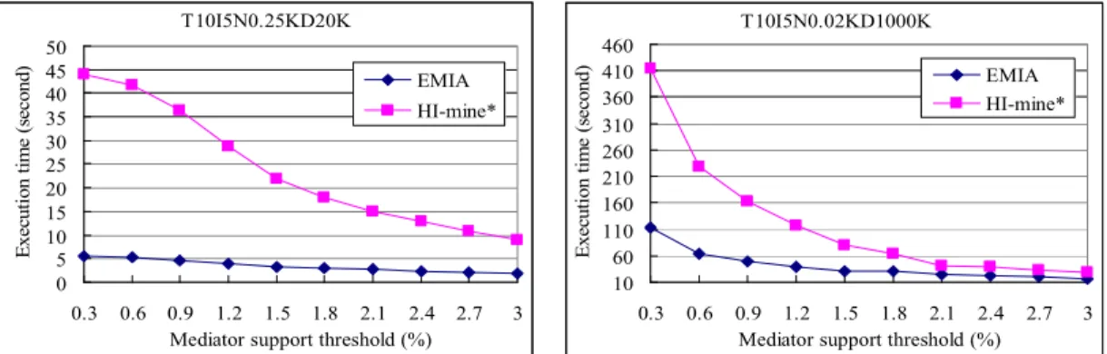
A. Evaluation on Synthetic Datasets

The performance curves of the datasets T10I5N0.25KD20K and T10I5N0.02KD1000K are depicted in Fig. 8. We can observe that the execution times of all algorithms are decreasing along with the increasing of mediator support (σf); EMIA is significantly superior to INDIRECT and also superior to HI-mine*, especially when the mediator support is small. Besides, INDIRECT is faster than HI-mine* when the mediator support threshold (σf) is greater than 0.03.

The memory usage comparison is shown in Fig. 9. In smaller dataset (10I5N0.25KD20K), the INDIRECT algorithm consumes the least memory but in the larger dataset (T10I5N0.02KD1000K) EMIA consumes the least.

There are two possible reasons. First INDIRECT does not need to keep all transactions in memory. Although algorithms EMIA and HI-mine* have adopted the compression technology, they still need larger memory to store the compressed transactions as compared with INDIRECT. Second, for EMIA and HI-mine* the dataset 10I5N0.25KD20K is composed of 250 items, resulting in relatively small ratio of analogical transactions. Therefore it is not easy to compress transactions. On the other hand, T10I5N0.02KD1000K contains only 20 items thus it is easier to be compressed, and so less memory is required. In addition, EMIA needs less memory than HI-mine* because EMIA adopts a relatively simple and efficient way in the projection phase.

B. Evaluation on Real Datasets

In this experiment, we evaluated the algorithms using real dataset. The execution time and memory usage comparisons are depicted in Figs 10 and 11, respectively. In summary from the results, the EMIA algorithm is the most efficient algorithm, and consumes approximately the same memory usage as HI-mine* but more memory than INDIRECT.

V. CONCLUSIONS

In this paper, we have proposed a new algorithm EMIA for mining indirect associations. Inspired by the success of HI-mine*, the EMIA algorithm adopts a more compact data structure and simple but more efficient way for indirect association generation. Experimental results on both synthetic and real world datasets have shown that EMIA is significantly faster than the leading algorithm Hi-mine* with comparable or less memory usage. In the future, we will

continue to improve the efficiency of the proposed algorithm, seeking more effective way for reducing the memory usage. We will also extend the proposed algorithm to the problem of stream data mining [1].

REFERENCES

[1] C. Aggarwal, Data Streams: Models and Algorithms, Springer, 2007. [2] R. Agrawal and R. Srikant, “Fast algorithms for mining association

rules in large databases,” Proc. of the 20th Intl. Conf. on Very Large Data Bases, pp. 487-499, 1994.

[3] L. Chen, S.S. Bhowmick, and J. Li, “Mining temporal indirect associations,” Proc. 10th Pacific-Asia Conference on Knowledge Discovery and Data Mining, Springer, Heidelberg, 2006, pp. 425-434. [4] P. Kazienko and K. Kuzminska, “The influence of indirect association rules on recommendation ranking lists,” Proc. 5th International Conference on Intelligent Systems Design and Applications, 2005, pp. 482-487.

[5] R. Kohavi, C. E. Brodley, B. Frasca, L. Mason, and Z. Zheng, “KDD-Cup 2000 organizers' report: peeling the onion,” SIGKDD Exploration Newsletters, vol. 2, pp. 86-93, 2000.

[6] A. Savasere, E. Omiecinski, and S.B. Navathe, “Mining for strong negative associations in a large database of customer transactions,” Proc. 4th International Conference on Data Engineering, pp. 494-502, 1998.

[7] C. Cornelis, P. Yan, X. Zhang, and G. Chen, “Mining positive and negative association rules from large databases,” Proc. IEEE International Conference on Cybernetics and Intelligent Systems, 2006, pp. 1-6.

[8] P. Kazienko, “IDRAM—Mining of indirect association rules,” Proc. International Conference on Intelligent Information Processing and Web Mining, 2005, pp. 77-86.

[9] R. Rymon, “Search through systematic set enumeration,” Proc. 3rd Intelligence Conference on Principles of Knowledge Representation and Reasoning, pp. 539-550, 1992.

[10] P.N. Tan, V. Kumar, J. Srivastava, “Indirect association: Mining higher order dependencies in data,” Proc. 4th European Conference Principles of Data Mining and Knowledge Discovery, 2000, pp. 632-637.

[11] P.N. Tan and V. Kumar, “Mining indirect associations in web data,” Proc. 3rd International Workshop on Mining Web Log Data Across All Customers Touch Points, 2001, pp.145-166.

[12] V.S. Tseng, Y.C. Liu, and J.W. Shin, “Mining gene expression data with indirect association rules,” Proc. National Computer Symposium, 2007.

[13] Q. Wan and A. An, ‘‘Efficient mining of indirect associations using

HI-mine,’’ Proc. 16th Conference of the Canadian Society for Computational Studies of Intelligence, 2003.

[14] Q. Wan and A. An, “An efficient approach to mining indirect associations,” Journal of Intelligent Information System, vol. 27, no. 2, pp. 135-158, 2006.

[15] Q. Wan and A. An, "Efficient indirect association discovery using compact transaction databases," Proc. of 2006 IEEE Intl. Conf. on Granular Computing, pp. 154-159, 2006.

[16] X. Wu, C. Zhang, and S. Zhang, “Efficient mining of both positive and negative association rules,” ACM Transaction on Information Systems, vol. 22, no. 3, pp. 381-405, 200

T10I5N0.25KD20K 0 5 10 15 20 25 30 35 40 45 50 0.3 0.6 0.9 1.2 1.5 1.8 2.1 2.4 2.7 3

Mediator support threshold (%)

E xe cu tio n ti m e (s ec on d) EMIA HI-mine* T10I5N0.02KD1000K 10 60 110 160 210 260 310 360 410 460 0.3 0.6 0.9 1.2 1.5 1.8 2.1 2.4 2.7 3

Mediator support threshold (%)

Exe cut ion t im e (s ec

ond) EMIA_HI-mine*

Figure 8. Execution time comparison on synthetic dataset.

T10I5N0.25KD20K 0 2 4 6 8 10 12 0.3 0.6 0.9 1.2 1.5 1.8 2.1 2.4 2.7 3

Mediator support threshold (%)

M em ory u sa ge (M B ) EMIA HI-mine* T10I5N0.02KD1000K 30 35 40 45 50 55 0.3 0.6 0.9 1.2 1.5 1.8 2.1 2.4 2.7 3

Mediator support threshold (%)

M em ory u sa ge (M B ) EMIA HI-mine*

Figure 9. Memory usage comparison on synthetic dataset.

BMS-WebView-2 0 200 400 600 800 1000 1200 1400 1600 1800 2000 0.3 0.6 0.9 1.2 1.5 1.8 2.1 2.4 2.7 3

Mediator support threshold (%)

E xe cu tion t im e ( se cond) EMIA HI-mine* BMS-POS 0 300 600 900 1200 1500 1800 2100 2400 2700 3000 0.3 0.6 0.9 1.2 1.5 1.8 2.1 2.4 2.7 3

Mediator support threshold (%)

E xe cu tion ti m e (s ec ond) EMIA HI-mine*

Figure 10. Execution time comparison on real dataset.

BMS-WebView-2 0 10 20 30 40 50 60 70 80 0.3 0.6 0.9 1.2 1.5 1.8 2.1 2.4 2.7 3

Mediator support threshold (%)

M em ory u sag e (M B ) EMIA HI-mine* BMS-POS 140 145 150 155 160 165 170 0.3 0.6 0.9 1.2 1.5 1.8 2.1 2.4 2.7 3

Mediator support threshold (%)

M em ory u sa ge (M B ) EMIA HI-mine*