使用粒子群最佳化於高優先權工作排程

全文

(1)國立交通大學資訊學院. 資訊學程. 碩士論文. 使用粒子群最佳化於高優先權工作排程. Particle Swarm Optimization for High Priority Job Scheduling. 研究生：邱文宏指導教授：孫春在. 教授. 中華民國九十六年六月.

(2) 使用粒子群最佳化於高優先權工作排程 Particle Swarm Optimization for High Priority Job Scheduling 研究生：邱文宏. Student：Wen-Hung Chiu. 指導教授：孫春在. Advisor：Chuen-Tsat Sun. 國立交通大學. 資訊學院. 資訊學程. 碩士論文. A Thesis Submitted to College of Computer Science National Chiao Tung University in Partial Fulfillment of the Requirements for the Degree of Master of Science in Computer Science June 2007 Hsinchu, Taiwan, Republic of China. 中華民國九十六年六月.

(3) 使用粒子群最佳化於高優先權工作排程 Abstract in Chinese 研究生：邱文宏. 國立交通大學. 指導教授：孫春在博士. 資訊學院. 摘. 資訊學程碩士班. 要. 在半導體廠中為了確保能夠及時完成有高時間性的批貨，便導入優先權的概念，以達成客戶的特殊需求，在最短的時間內讓產品上市。雖然高優先權的工作同時也代表較高的利潤，但也同時為半導體廠設備的生產量帶來不良的影響。在半導體廠中一般的做法是把設備切換至待機模式，等待高優先權的批貨到達設備輸入端，以減少處理高優先權批貨的延誤並確保批貨儘快完成處理。但是如此一來設備是在妥善的狀態卻不能執行工作，設備的使用率便因此降低。半導體廠設備多半非常昂貴，所以半導體設備的使用率一直都是半導體廠中重要的課題。為了提高半導體設備的使用率，我們提出一個適用於半導體設備工作排程，易於實現，有效而且快速的粒子群最佳化演算法。實驗的結果顯示這個修改過的方法確實有效率，運算快速而且容易實現。即使在現階段此方法有條件限制，它的成效是比原本的粒子群最佳化應用要來得高的，而且在小數量的工作排程上的確效果顯著。. 關鍵字：工作排程、人工智能、粒子群最佳化. -i-.

(4) Particle Swarm Optimization for High Priority Job Scheduling. Student：Wen-Hung Chiu. Advisor：Dr. Chuen-Tsat Sun. Degree Program of Computer Science National Chiao Tung University. Abstract High Priority Lot is a measure taken in Semiconductor Fabrication manufactory to ensure on-time delivery of high time-sensitive lots to cope with device maker’s need for prompt delivery of their high-tech products. Although High Priority Lot can bring higher profit to the factory, it also has bad influence on equipment throughput. It is common practice that the equipment is switch to idle mode and waits for the arrival of High Priority Lot in order to guarantee minimum delay. However, this impacts the utilization of the equipment, for the equipment is fully functional but doing nothing while waiting for the High Priority Lot. Manufacturing equipment is extremely expensive so that maximizing the utilization of the equipment has became an important topic in semiconductor fabrication manufactory.. In order to improve equipment utilization, we propose a modified PSO application that is easy to implement, effective and fast in scheduling jobs on semiconductor. - ii -.

(5) equipment by redefining the search space. The results indicate that the method is efficient, fast and easy to implement. The performance is better than the original PSO application, especially for job scheduling with small job count, even though there are limitations in current stage of the research.. Keywords: Job scheduling, Artificial Intelligence, Particle Swarm Optimization. - iii -.

(6) 誌. 謝. Acknowledgement in Chinese 在美國工作六年，回到台灣後一直渴望能再回學校進修，再次踏入校園，兩年的日子中，能夠選讀自己感興趣的課目與作研究，內心的感動無法言喻。首先誠摯的感謝指導教授孫春在博士，老師的教導讓我得以進一步瞭解人工智能的技術，不厭其煩的指點我研究的方向，使得此篇論文能夠順利完成。同時也要感謝我的論文口試委員張智星教授與胡毓志教授，給予許多寶貴的意見，讓此篇論文的內容更為精確嚴謹。感謝朝淵學長不時的指出我研究中的缺失，也感謝碧如給了我很多有用的意見，使得本論文的實驗能夠更完整。也感謝各位同學的幫忙順利修完這兩年的課程，大家共同學習、討論、趕作業的情景都是我畢生難忘的經驗。由衷的感謝我的妻子淑玲在背後默默的支持我，沒有淑玲的體諒、包容，相信我沒辦法安心的修課跟作研究。也感謝我的兩個兒子品富與品詮為我忙碌的生活帶來歡樂與喜悅。最後，感謝我摯愛的雙親邱火淵及邱戴彥芬對我的栽培與諄諄教誨。. - iv -.

(7) Acknowledgement in Chinese. Contents Abstract in Chinese ..................................................................................... i Abstract ...................................................................................................... ii Acknowledgement in Chinese .................................................................. iv Contents ......................................................................................................v List of Figures .......................................................................................... vii List of Tables........................................................................................... viii Chapter 1 Introduction and Motivation ......................................................1 1.1 Backgrounds ......................................................................................1 1.2 Motivations........................................................................................3 1.3 Scheduling problems .........................................................................5 Chapter 2 Related Works ............................................................................8 2.1 Heuristic Algorithm...........................................................................8 2.2 Genetic Algorithm .............................................................................9 2.3 Particle Swarm Optimization for Scheduling Problem...................10 2.4 Comparison between GA and PSO .................................................12 Chapter 3 One-Dimensional PSO and Experiments.................................14 3.1 Original PSO Approach...................................................................14 3.2 Proposed One-Dimensional PSO ....................................................18 3.2.1 Finding all possible permutations .............................................19 3.2.2 Find the optimal permutation....................................................21 3.2.3 Perform PSO operations ...........................................................21 3.3 Fitness function for High priority Lot Scheduling Problem ...........22 3.4 Performance Evaluation ..................................................................24 Chapter 4 Results ......................................................................................26 -v-.

(8) 4.1 Fitness Distributions........................................................................26 4.2 Search Result Distributions.............................................................29 4.3 Convergence Trend..........................................................................31 4.4 Success Rate ....................................................................................33 4.5 Computational Cost Evaluations.....................................................34 Chapter 5 Conclusions and Future Works ................................................38 References.................................................................................................41 Appendix A: Job Sets Used for Experiments ...........................................44 Appendix B: 9 Jobs Search Results ..........................................................47 Appendix C: 8 Jobs Converge Trend Data ...............................................49 Vita ............................................................................................................51. - vi -.

(9) List of Figures FIGURE 1-1 FACTORY OUTPUT IMPACT BY HIGH PRIORITY LOT ....................2 FIGURE 1-2 INSERTING PRIORITY JOBS.........................................................4 FIGURE 1-3 SCHEDULES WITH HIGH PRIORITY LOT .....................................6 FIGURE 2-1 FLOW DIAGRAM OF GENETIC ALGORITHM ..............................10 FIGURE 3-1 RESULTS OF DIFFERENT LOCATIONS .........................................15 FIGURE 3-2 CALCULATION OF PARTICLE VECTORS......................................17 FIGURE 3-3 FLOW DIAGRAM OF PARTICLE SWARM OPTIMIZATION.............18 FIGURE 3-4 SEARCH SPACE OF ONE DIMENSION PSO................................22 FIGURE 4-1 TWO-DIMENSIONAL SEARCH SPACE EXAMPLE .........................26 FIGURE 4-2 ONE-DIMENSIONAL SEARCH SPACE ..........................................27 FIGURE 4-3 ONE-DIMENSIONAL SEARCH SPACE WITH PRE-CALCULATED PERMUTATIONS ....................................................................................28. FIGURE 4-4 ONE-DIMENSIONAL SEARCH SPACE WITH RUNTIME-CALCULATED PERMUTATIONS ....................................................................................29. FIGURE 4-5 SEARCH RESULT DISTRIBUTIONS OF ORIGINAL PSO (9 JOBS) .30 FIGURE 4-6 FITNESS DISTRIBUTIONS OF ONE-DIMENSIONAL PSO (9 JOBS) ............................................................................................................31 FIGURE 4-7 CONVERGENCE TREND (8 JOBS) .............................................32 FIGURE 4-8 COMPARISON OF COMPUTATIONAL COST ................................36. -vii-.

(10) List of Tables TABLE 2-1 COMPARISONS BETWEEN PSO AND GA ....................................12 TABLE 3-1 SAMPLE JOB RANKINGS (5 JOBS)..............................................15 TABLE 3-2 SAMPLE PERMUTATIONS (4 JOBS).............................................21 TABLE 4-1 SUCCESS RATE ..........................................................................33 TABLE 4-2 COMPUTATIONAL COST FOR CALCULATING 5,100 ITERATIONS .35 TABLE 4-3 TIME COMPLEXITY OF EACH CALCULATION..............................37. -viii-.

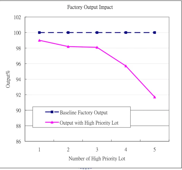
(11) Chapter 1 Introduction and Motivation. 1.1 Backgrounds. As the competitions in high-tech products grow, it is important to bring the products to the buyers in the shortest period of time. In order to cope with device maker’s need for fast delivery, lot priority was introduced to semiconductor fabrication manufactories [1][2][3].. High Priority Lot has been an important topic in semiconductor manufacturing as these lots have higher priorities than other lots and will impact the performance of individual semiconductor equipments and the whole semiconductor fabrication manufactory. HPL (High Priority Lots) impacts equipments since the equipment usually waits for the arrival of HPL. As a result, the performance of the whole factory is degraded as shown in Figure 1-1 [1].. -1-.

(12) Factory Output Impact 102 100 98. Output%. 96 94 92 90. Baseline Factory Output Output with High Priority Lot. 88 86 1. 2. 3. 4. 5. Number of High Priority Lot. Figure 1-1 Factory output impact by High Priority Lot. Equipment task scheduling becomes an active research area in hope to improve the performance of a semiconductor manufactory [1][4][5]. In this thesis, we will discuss how to improve the performance of individual equipment and attempt to help to relief the performance impact caused by inserting High Priority Lots.. -2-.

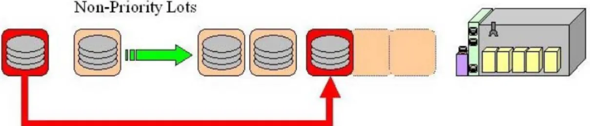
(13) 1.2 Motivations. Taking the wet bench (chemical bath) equipment as an example, the equipment is often composed of several processing modules, at least one Front Opening Unified Pod (FOUP) input/output unit and an internal buffer for storing FOUPs to be processed. The processing modules contain different types of chemical liquid (pure or mixed) or de-ionized water. The wafers are usually taken out of the FOUP and dipped in different chemicals and/or dried depending on selected recipes. The wafers can stay in a bath, the containers that contain the chemical liquid, for different length of time up to tens of minutes. In normal practice, the lots are processed in a First-Come-First-Serve (FCFS) order since it is the simplest way to implement a scheduler. High Priority Lots (HPL), on the other hand, has the highest priority and usually causing the equipment to stop processing non-priority jobs. When the equipment is expecting a HPL, it may be placed in idle mode for hours and waits for the arrival of HPL. When the HPL arrives, the equipment will then serve the HPL first before continuing to serve the non-priority lots, as shown in Figure 1-2.. -3-.

(14) Figure 1-2 Inserting Priority Jobs. This is done to ensure that HPL will be processed as soon as it arrives at the equipment, as it is the simplest way and with lowest cost for equipment implementation. However the velocity of none-priority lots are affected [1]. There are also other factors that contribute to the decrease of equipment throughput, such as scheduled down/maintenance time, but are not discussed in this paper. The length of idle time waiting for HPL will make the throughput of the equipment degrade dramatically as the equipment is fully functional but cannot be used to process any wafers while waiting.. In order to reduce the effect of throughput degradation, we can attempt to process jobs while the equipment is waiting for the arrival of Supper Hot Lot. If we. -4-.

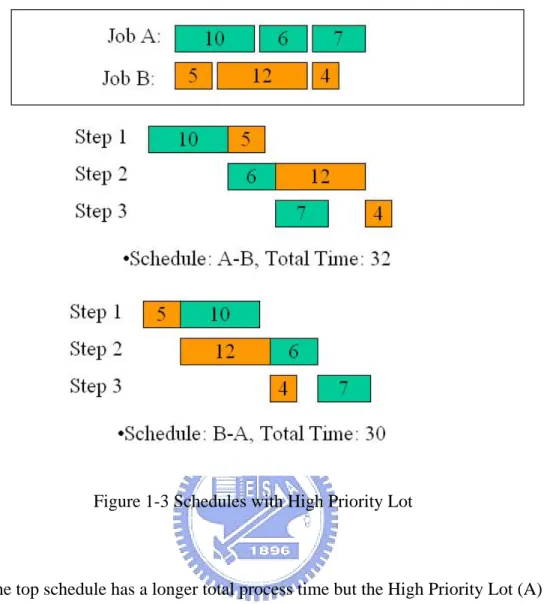
(15) can send HPL related information, such as estimated arrival time or latest finish time, to the equipment through factory automation host using messages defined in SEMI standards [6][7], then we may be able to have some non-priority jobs to be processed before HPL arrives as long as it does not cause delays on the finish time of HPL. This not only requires in depth knowledge of the manufacturing processes but also an easy to implement and efficient scheduler with acceptable performance for the respective equipments to achieve optimal utilization.. 1.3 Scheduling problems. A scheduler decides the order of lots to be processed. Two different schedules may result in different total process time. However, the fitness of a schedule not only depends on the total process time but also needs to take the process end time of High Priority Lots into consideration since we get penalties if the High Priority Lot does not finish by the expected deadline, as shown in Figure 1-3.. -5-.

(16) Figure 1-3 Schedules with High Priority Lot. The top schedule has a longer total process time but the High Priority Lot (A) is finished 23s after the process starts. In the other schedule, the High Priority Lot is finished 30s after the process starts, which may be a problem if the deadline for High Priority Lot is between 23s and 30s even though the schedule has a shorter total process time.. As numbers of unprocessed job increases, it becomes more difficult for the scheduler to find the optimal solution/permutation that has the shortest total process time or best fitness since the possible permutations of the jobs increase exponentially, -6-.

(17) which sometimes make doing an exhaustive search computationally impossible [8]. This is classified as a NP-Hard problem (Stephen A. Cook, 1971) [9].. There are different methodologies that can be applied to find solutions to a scheduling problem. For example, Genetic Algorithm (GA), Swarm Intelligence (SI) and even Knowledge based system methods. Most of these methods attempt to find an “acceptable” solution instead of the optimal solution, as the search space is often too large to be searched thoroughly. Most of the time, a budget (fixed period of time or fixed number of iterations) is defined to be used before the calculation converges and just settle for the best solution found in the process. In order to cope with the need for a simple, fast and efficient scheduler for semiconductor equipment, we introduce a modified Particle Swam Optimization method that is well suited for small to mid size job number on semiconductor equipment. In Chapter 2, related works on solving scheduling problems are introduced. Chapter 3 presents the proposed method, a one-dimensional PSO search. The experiments are described in Chapter 4 and the conclusions and future works in Chapter 5.. -7-.

(18) Chapter 2 Related Works. Scheduling is a complex problem that we encounter in semiconductor fabrication factories everyday. Various methodologies are used in an attempt to look for the optimal solution. Among these methods, Genetic Algorithm (GA) [10][11] and Swarm Intelligence methods [12][13][14], each has its’ advantages and disadvantages. We will introduce and discuss these methods in this chapter.. 2.1 Heuristic Algorithm. Heuristic algorithm is a methodology that has been proven to find a near optimum solution in a reasonable time. It searches down the path of a search tree and determines the distance to the initial state during the progress and attempts to estimate the distance between the goal and current state using the heuristic functions in order to improve its searching efficiency. It is often used in semiconductor manufactories for lot scheduling due to its efficiency in calculation [15]. Sometimes simplified logical rules, that are designed closely related to the factory operation, are used in order to reduce the complexity.. -8-.

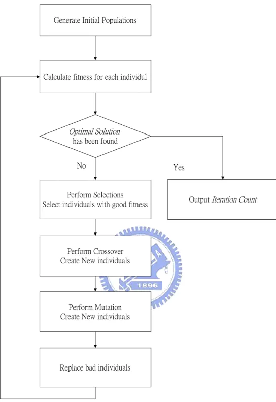
(19) 2.2 Genetic Algorithm. Genetic Algorithm was invented in 1970 based on the theory of evolutions and genetics of life forms. Inheritance and crossover of parent solutions creates new generations. Since the good genes survive and bad ones will be eliminated through competition, the descendents usually produce better fitness. However, this method tends to converge with local optimum. Mutation of the genes ensures diversity of child generations. Thus we have a better chance in evolving to a better (if not the best) solution. Typically a solution is presented as a bit array. Depends on the nature of the problem a fitness function (sometimes called a cost function) is defined to compare the solutions quantitatively [16]. In typical implementation of GA for scheduling problem, we use a string consists of all job IDs to represent a solution. The order of jobs in the string indicates the order in which the jobs will be processed.. Initial population is generated randomly. Parents are selected and perform crossover to generate the next generation. Mutations are conducted randomly to diversify the new population. The process is shown in Figure 2-1.. -9-.

(20) Generate Initial Populations. Calculate fitness for each individul. Optimal Solution has been found No. Yes. Perform Selections Select individuals with good fitness. Output Iteration Count. Perform Crossover Create New individuals. Perform Mutation Create New individuals. Replace bad individuals. Figure 2-1 Flow Diagram of Genetic Algorithm. 2.3 Particle Swarm Optimization for Scheduling Problem. Particle Swarm Optimization is one of Swarm Intelligence methods. It was -10-.

(21) introduced by J. Kennedy and R. Eberhart in 1995 [17][18]. The methodology has been proven to be successful in solving optimization problems on various continuous functions [19]. The idea was inspired by observing the foraging of bird flocks. The behavior of an individual in a swarm not only depends on its own knowledge but also affected by the behavior or knowledge of other individuals in the swarm. For example, when one individual in the swarm or herd finds food in its path, the others will head toward that direction even if they don’t previously have the knowledge of that location. Also, other entities in the swarm do not simply head for the location that has food. It is common that they often veer off the path randomly and find food elsewhere. This also ensures that other locations in the search space are randomly searched.. When modeling such a swarm, particles are introduced to represent an individual in the swarm. A random location is selected and assigned to each particle. A fitness function is defined to evaluate the solutions represented by these locations. Each particle has an initial speed in each dimension of the search space. The particles then move in the space base on the memory of its own experience on best-known location and the swarm’s best-known location.. - 11-.

(22) Similar to mutation that is used in GA a random factor is introduced in deciding the movement of a particle. It is important as it diversify the swarm. The fitness is calculated for the new locations and then new vectors and directions are calculated for each particle.. 2.4 Comparison between GA and PSO. GA and PSO have very different features and behavior. Table 2-1 gives a list of the differences between GA and PSO.. Table 2-1 Comparisons between PSO and GA. PSO. GA. Search Space. Continuous. Discrete. Survival. All Particles Survives. Fittest Population. Knowledge on past results pbest and gbest. Parents. Searching Behavior. Directional. Omnidirectional. Diversity. Random Coefficients. Mutation. The two methodologies look fairly similar in some ways. They both preserve. -12-.

(23) the good results and have a way to diversify the population. PSO has a very obvious direction in its searching process. It is moving toward the past locations with best solutions. GA seems to be searching in all direction. It is mainly because the search space is discrete and it is the nature of the methodology.. GA has a discrete search space that no close relationship associated between different solutions. PSO implementation has a continuous search space and neighboring permutations usually have similar fitness.. Another big difference is survival of entities in the population. Solutions in the population with better fitness are selected to generate new generations while others are retired from the population. Unlike GA, all particles in PSO will survive and live until the end of the process.. -13-.

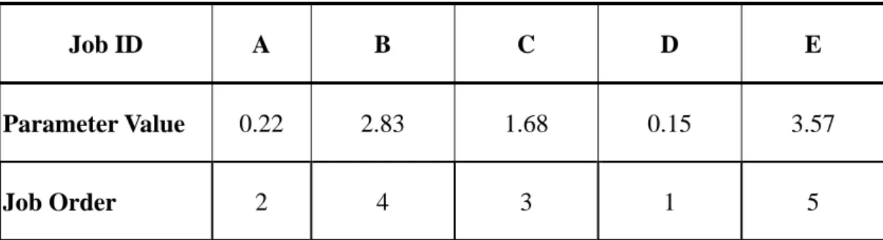
(24) Chapter 3 One-Dimensional PSO and Experiments. In this chapter we will introduce the proposed method, a modified PSO application. In order to evaluate the performance of the proposed method, we will attempt to find the optimal solutions using the simulators with original PSO application. We will discuss how different methodologies are implemented and how experiments are done. The job sets used in the experiments are created randomly as shown in Appendix A.. 3.1 Original PSO Approach. In practical PSO implementation for scheduling problems, each job in the job pool is represented as a dimension. A position of a particle consists of one parameter (rank) for each dimension; here is an example in Table 3-1.. -14-.

(25) Table 3-1 Sample Job Rankings (5 Jobs). Job ID Parameter Value Job Order. A. B. C. D. E. 0.22. 2.83. 1.68. 0.15. 3.57. 2. 4. 3. 1. 5. Base on the ranks of the dimensions, an order is decided and the fitness can be calculated. However, different locations in the search space may present the same solution as shown in Figure 3-1.. Figure 3-1 Results of different locations. -15-.

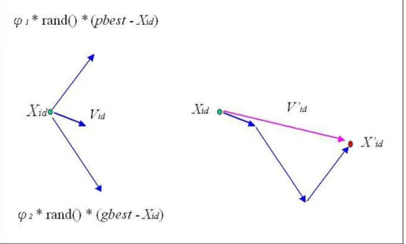
(26) We use a string consists of all job ID to present a solution and each location in the search space presents one solution. The order of jobs in the string indicates the order in which the jobs will be processed. Initial positions for a fixed number of particles are selected randomly and the fitness of these positions is calculated.. The vector Vid of each dimension of a particle is then calculated with current position xid , the best-known position in the swarm p gd , best-known position of particle pid , acceleration coefficients c1 and c 2 , w the inertia factor and random numbers Rand1 and Rand 2 using equation (1), and equation (2) calculates the new position:. Vid = w × Vid + c1 × Rand1 () × ( pid − xid ) + c2 × Rand 2 () × ( p gd − xid ). (1). xid = xid + Vid. (2). Figure 3-2 shows how the new vector is composed. This process is performed for each dimension that define the position of a particle.. -16-.

(27) Figure 3-2 Calculation of particle vectors. In order to simplify the experiment and focus on the differences between the original and the modified methods, we set w to constant 1 for both methods and C1 and C2 are set to 2.05 as recommended by previous study [21].. The process is repeated until the criteria for termination is met. The flow diagram is shown in Figure 3-3.. -17-.

(28) Initialize Seed Particles. Calculate fitness and Update pbest and gbest. Criteria for termination is met. Yes. No. Calculate Particle velocity and direction using PSO operations. Output gbest. Update Particle Locations. Figure 3-3 Flow Diagram of Particle Swarm Optimization. 3.2 Proposed One-Dimensional PSO. In semiconductor fabrication manufactories, we usually do not assign a large amount of jobs to an equipment at a time. In the case of wet-bench equipment, the typical maximum jobs allowed ranges from 8 to 18 jobs depending on the size of the buffer area. There are 10 buffer locations in the equipment that we are using as a model for the experiment. In order to increase the equipment utilization, a fast and. -18-.

(29) reliable scheduler is needed to quickly find the best or optimal schedule. We propose a modified Particle Swarm Optimization method to be used on the equipment in order to find the best or acceptable schedule in a simple and less time consuming (comparing with the original PSO method) fashion. The process for calculating the next position for particles is similar to original PSO except that the search space is converted from a N-dimensional space to a one-dimensional space.. 3.2.1 Finding all possible permutations. Instead of using rankings for each job, we use an index to represent a permutation. The permutations of all jobs are determined in advance and lined up to form a one-dimensional space. The permutations can be pre-calculated or calculated at runtime. It is designed so that the adjacent permutations have somewhat similar fitness in order for the PSO search to be most effective.. Simply use a recursive function to generate all the permutations. Every permutation is unique and only differs from the neighboring permutations on two job positions as shown in Table 3-2. However, it becomes time consuming and requires lots of space to store the permutations when the job count gets bigger. Bellow is the pseudo code for generating the permutations: -19-.

(30) GeneratePermutations() { Initialize Job IDs; Compose the first permutation; reset used JobID count to 0; Call DoChild(Initial Job permutation, 0) } DoChild(JobStr, Used JobID Count) { For each JobIDs that is unused { If only one unused JobID left then Output the resulted permutation Else { Set next JobID in string as used Call DoChild(JobStr, used JobID count +1) If found the position of next unsed JobID then Swap next JobID with the used JobID } } }. -20-.

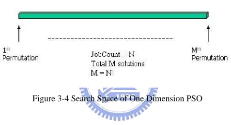
(31) Table 3-2 Sample Permutations (4 Jobs). Index Permutation Index Permutation Index Permutation Index Permutation 1. ABCD. 7. CABD. 13. BCAD. 19. DACB. 2. ABDC. 8. CADB. 14. BCDA. 20. DABC. 3. ADBC. 9. CDAB. 15. BDCA. 21. DBAC. 4. ADCB. 10. CDBA. 16. BDAC. 22. DBCA. 5. ACDB. 11. CBDA. 17. BADC. 23. DCBA. 6. ACBD. 12. CBAD. 18. BACD. 24. DCAB. 3.2.2 Find the optimal permutation. In order to evaluate the performance and success rate of each method, we also calculate the fitness for every single solutions/permutations using brute force method. Similar to generating all possible permutations, this again can be very time consuming when job count gets bigger and bigger. We will do up to 10 jobs in the experiments.. 3.2.3 Perform PSO operations. Once the permutations are created and lined up to form a line, we can deploy PSO operations in the new search space. As shown in Figure 3-4, basically, we are. -21-.

(32) now searching in a one-dimensional space instead of the N-dimensional continuous space in the original PSO method [12]. We search the space for optimal solution for a fixed number of iterations and evaluate the performance of each method.. Figure 3-4 Search Space of One Dimension PSO. Based on previous study [21], the recommended particle size is 30 particles for general purpose. We initialize 30 particles and calculate the vectors of the particles with recommended factors.. 3.3 Fitness function for High priority Lot Scheduling Problem. Fitness function is the major difference that distinguishes High Priority Lot (HPL) scheduling from other scheduling problems. When HPL is involved, we not. -22-.

(33) only need to consider the total process time but also the finish time of HPL. Since the fitness function varies depends on different preferences of the implementations, we had designed a fitness function that combines total process time and delay time of HPL. Because the delay of HPL will result in penalties, we multiply the HPL delay time by 3, and use the sum of the weighted delay time and total process time as new fitness, if HPL is overdue in a solution. This may not necessary reflect the real life factory practice but gives a taste of how these factors are taken into consideration and how they affect the resulted fitness.. The fitness function is described as follows: Each of the n jobs has m steps and. The processing time of jth step of ith job is given as Pi,j. The completion time jth step of job i is denoted as C(i,j). Assume all steps use different equipment resources so that the equipment can simultaneously process m steps. The following equations (1)(2) denotes the fitness function similar to [14]:. i = 2, K , n;. C (1, 1 ) = P1 , 1. k = 2,K , m (3). C ( i ,1 ) = C ( i − 1, 1 ) + Pi ,1. (4). C (1, k ) = C ( i − 1, k − 1) + P1 , k. (5 ). C ( i , k ) = max {C ( i − 1, k ), C ( i , k − 1 ) } + Pi , k Fitness. = C (n, m ). -23-. (6 ).

(34) In order to take into account the effect of delay on HPL, the fitness function needs to be further adjusted. Assuming the 3rd job is HPL and deadline is twice the shortest completion time of the HPL and the penalty for delay is the length of the delay times 5. The adjusted fitness function is denoted as follows:. ⎧ ⎪⎪ C ( n , m ) Fitness = ⎨ k ⎪ C ( n , m ) + 5 × ( C ( 3 , m ) − 2 × ∑ P3 , j ) ⎪⎩ j =1. k. , if C ( 3 , m ) <= 2 × ∑ P3 , j j =1. k. , if C ( 3 , m ) > 2 × ∑ P3 , j j =1. 3.4 Performance Evaluation. The performance and behavior of the proposed methodology is evaluated under the following conditions:. 3~10 jobs are randomly generated. Each job has three steps with randomly generated processing time.. A test run consists of initiations of particles, 20 iterations of PSO operations (particle movements). The test is repeated 10000 times and the following characteristics are analyzed.. -24-.

(35) Permutation Fitness Distribution Search Result Distributions Convergence Speed Success Rate Computational Cost. -25-.

(36) Chapter 4 Results 4.1 Fitness Distributions. When applied to batch processing scheduling, the original Particle Swarm Optimization is searching in a N-dimensional space, where N is the number of jobs to be scheduled. This creates a big search space and results in multiple particle locations representing the same solution. As shown in Figure 4-1, is an example of a two-dimensional search space [22].. Figure 4-1 Two-dimensional search space example. The proposed method searches in a one-dimensional search space as shown in. -26-.

(37) Figure 4-2. In this example, there are 5 jobs to be scheduled and assumes no High Priority Lot. There are total of 120 different permutations.. 5 Job Fitness Distributions without High Priority Lot 600. Fitness (sec). 500 400 300 200 100 0 1. 11. 21. 31. 41. 51. 61. 71. 81. 91. 101. 111. Permutation Index. Figure 4-2 One-dimensional search space. A one-dimensional search space has many advantages including a finite discrete search space, unique permutation per location. For a particle in a one-dimensional PSO search, it is likely to engage more local optimum than in the original PSO. While local optima are also candidates of the global optimum, it appears that one-dimensional PSO has a better chance of finding the global. -27-.

(38) optimum.. When High Priority Lot is introduced to the job set, the distributions of the fitness becomes less smooth creating more hills as shown in Figure 4-3. This affects the search spaces for both original PSO and the proposed method.. 5 Job Fitness Distributions with High Priority Lot (Pre-Calculated Permutations) 2500. Fitness (sec). 2000 1500 1000 500 0 1. 11. 21. 31. 41. 51. 61. 71. 81. 91. 101. 111. Permutation Index. Figure 4-3 One-dimensional search space with pre-calculated permutations. The permutations can also be created at runtime. However, the permutations created by this approach, as shown in Figure 4-4, do not line up as well as the permutations created using pre-calculated method so it appears to have created more -28-.

(39) humps than the pre-calculated permutation set.. 5 Job Fitness Distributions with High Priority Lot (Permutation Calculated at Runtime) 2500. Fitness (sec). 2000 1500 1000 500 0 1. 11. 21. 31. 41. 51. 61. 71. 81. 91. 101. 111. Permutation Index. Figure 4-4 One-dimensional search space with runtime-calculated permutations. 4.2 Search Result Distributions. Next we will analyze the distribution of the search results of the methods. The data is collected using the job set of 9 jobs case after 255 repetitions (see Appendix B for data set). The distributions of the search result will also show the differences between the methods. As shown in Figure 4-5, the original PSO converges more concentrated at 566 (over 200 hits). -29-.

(40) Figure 4-5 Search Result distributions of Original PSO (9 Jobs). One-dimensional PSO has a more scattered distribution and, in this particular case, it is able to find the global optimum fitness (562) as shown in Figure 4-6. This seems to imply that one-dimensional PSO searched a wider area in the search space thus better chance of finding the global optimum.. -30-.

(41) Figure 4-6 Fitness distributions of One-Dimensional PSO (9 Jobs). 4.3 Convergence Trend. The convergence trend is difficult to evaluate as it highly depends on the initial locations of the particles. There are also researches in this area [23]. In this thesis, we collected data that use the job set of 8 jobs case. We handpicked data where all three methods have similar fitness at initialization, as shown in Appendix C. An example is shown in Figure 4-7. (One-dimensional PSO uses pre-calculated and One-dimensional PSO II uses runtime-calculated permutation set.) We found that the original PSO tend to converge faster than one-dimensional PSO and the two. -31-.

(42) one-dimensional PSO methods has similar converge characteristics.. Converge Trend 505 500. One-Dimensional PSO. Best Fitness (sec). 495. One-Dimensional PSO II. 490 485 480 475 470 465. 49. 45. 41. 37. 33. 29. 25. 21. 17. 13. 9. 5. 1. 460 Repetition Index. Figure 4-7 Convergence Trend (8 Jobs). However, slower convergence speed is not necessarily bad. In fact, this is consistent with our earlier findings. The original PSO converges faster since there are less local optimums in the moving path of a particle. The one-dimensional PSO has a finite discrete search space without duplicated permutations so a particle engages more local optimums as they move toward the target. That is why the. -32-.

(43) one-dimensional PSO appears to have a slower convergence speed.. 4.4 Success Rate. Success rate is an important indication of the performance of a method. We ran each method for 10,000 repetitions and calculate the success rate by dividing the number of times global optimum found by the number of repetitions (10,000). The results are shown in Table 4-1.. Table 4-1 Success Rate Job Count. N-Dimensional (Original). 1-Dimensional (Pre-calculated). 1-Dimensional (Runtime). 3. 100%. 100%. 100%. 4. 99.6%. 100%. 100%. 5. 97.8%. 99.4%. 99.2%. 6. 93.0%. 93.4%. 99.0%. 7. 32.4%. 29.7%. 45.2%. 8. 5.2%. 1.6%. 2.8%. 9. 0.09%. 0.16%. 0.15%. 10. 0.26%. 0.13%. 0.29%. -33-.

(44) As the results show, the success rate start to fall when there are four jobs in the job pool when using original N-dimensional PSO. One-dimensional PSO still have 99% success rate when there are 6 jobs. Also one-dimensional PSO has better success rates in almost all cases tested. The interesting thing is that, at eight jobs, N-dimensional PSO outperforms one-dimensional PSO. We believe that this is an example the shows that location of global optimum does effect the success rate. Original N-dimensional PSO will have advantage over one-dimensional PSO if the global optimum is located near the center of the search space.. 4.5 Computational Cost Evaluations. We also calculated the time spent for performing same amount of iterations using different methodologies. Computational cost here is defined by the time duration for calculating 5,100 iterations (255 repetitions) of each method on the same computer, as shown in Table 4-2.. -34-.

(45) Table 4-2 Computational Cost for Calculating 5,100 Iterations Job Count. 3. 4. 5. 6. 7. 8. 9. 10. 1-D PSO (sec). 3.5. 4.6. 3.5. 5.8. 5.8. 5.8. 6.9. 6.9. 1-D PSO II (sec). 4.6. 4.6. 6.9. 5.8. 8.1. 8.1. 9.3. 10.4. Original PSO (sec). 5.8. 6.9. 9.3. 11.6. 12.7. 13.9. 16.2. 18.5. The differences may look insignificant when the job count is small. As the job count increases to 10, the cost for original PSO is almost twice the cost of one-dimensional PSO using runtime-calculated permutation and is over 2.5 times the cost of one-dimensional PSO using pre-calculated permutation as shown in Figure 4-8.. -35-.

(46) Time Duration for Calculating 5,100 Iterations One-Dimensional PSO. One-Dimensional PSO II. Original PSO. 20 18 16. Duration (sec). 14 12 10 8 6 4 2 0. 31. 42. 35. 64. 57. 68. 79. 10 8. Job Count. Figure 4-8 Comparison of Computational Cost. By analyzing the time complexity of each operation during the process, it is not difficult to realize why one-dimensional PSO will outperform N-dimensional PSO. The calculations are separated into three phases: Generation of Permutation, Fitness Calculation and Location Change for analysis as shown in Table 4-3.. -36-.

(47) Table 4-3 Time Complexity of each Calculation Calculations. N-Dimensional (Original). 1-Dimensional (Pre-Calculated). 1-Dimensional (Runtime). Permutation. O (N log N). O (1). O (N). Fitness. O (N). O (N). O (N). Location. O (N). O (1). O (1). The cost for fitness calculating depends on number of jobs in the job pool. It makes no difference between different approaches.. For N-dimensional PSO, sorting algorithm is required to sort the job ranks in order to generate a permutation. In this thesis, we select quick sort for sorting the values and the time complexity of quick sort is O (N log N). One-dimensional PSO does not require sorting. The time complexity is a constant if the permutation is previously calculated and O (N) if calculated at runtime.. As for calculating new particle location, since the location of a particle is fixed by N dimensions in original PSO application, the PSO particle movement operations need to be performed N times while we only do it one time when one-dimensional PSO is used.. -37-.

(48) Chapter 5 Conclusions and Future Works. The goal of this research is to find a methodology that is designed to fit the need of a semiconductor equipment scheduler. As a result of the experiments, we found that the proposed method has very good performance for scheduling job numbers range between 3 and 10. It is capable of finding the global optimum quickly and efficiently. It has a better success rate than the original PSO in tested cases.. As the job count gets bigger, the method that uses pre-calculated permutations starts to show its limitation. The resources required for storing the permutations increase exponentially and may be impossible to store all possible permutations. Using runtime-calculated permutations will help relief the problem with slightly decreased performance.. There are lots of differences between one-dimensional PSO and the original PSO in terms of the behavior and performance. Performance-wise, one-dimensional PSO has advantage over original PSO as it uses only simple calculation to create the permutation, while original PSO requires a sorting mechanism, which is -38-.

(49) computationally expensive to sort the rankings of each job in order to create the permutation. Furthermore, the time for calculating the schedule increases dramatically as job count grows.. The behaviors of the methods are also very different. By looking at the converging trend, it looks as if original PSO is converging quickly and much faster than the method proposed. However, the true meaning is that, using proposed method, we are able to search the search space more thoroughly as the search space has been reduced to a finite discrete space without duplicated permutations. This enables us to find more local optimums. In other words, it is more likely to find the global optimum. Each method has its advantage and is up to the user to choose between possibilities of finding global optimum or shorter converging time.. There are a few areas that we can further study. The method that we used to generate permutations is not the only method. We believe that there are other methods for creating the permutation set. We may be able to find a better function for constructing a search space with smoother fitness distribution line and resulting in better search results. We believe that optimizing the particle initializations and changing number of iterations can also improve the success rate.. -39-.

(50) It is obvious that the one-dimensional PSO is suitable for combinatorial problems. Since we have converted the search space to a one-dimensional search space, we may be able to apply one-dimensional optimization methodologies to solve the scheduling problem more efficiently. These are works that we believe to be worth further exploration.. -40-.

(51) References [1] Chad D. DeJong and Scott P. Wu, “Simulating the Transport and Scheduling of Priority Lots in Semiconductor Factories”, Proceedings of the 34th Winter Simulation Conference, Session: Semiconductor Manufacturing, pp. 1387-1391, 2002. [2] Linda F. Atherton and Robert W. Atherton, Wafer Fabrication: Factory Performance and Analysis, Kluwer Academic Publishers, 1995. [3] Russ M. Dabbas and John W. Fowler, “A New Scheduling Approach Using Combined Dispatching Criteria in Wafer Fabs”, IEEE Trans. On Semiconductor Manufacturing, Vol.16, No.3, pp.501-510, August 2003. [4] Mike Hillis and Jennifer Robinson, “Extremely Hot Lots: Super-Expediting in a 0.18 Micron Wafer Fab”, Proceedings of the MASM Conference, 2002. [5] Asbjoern M. Bonvik, “Estimating the Lead Time Distribution of Priority Lots in a Semiconductor Factory”, Operations Research Center Working Papers, Massachusetts Institute of Technology, Operations Research Center, May 1994. [6] SEMI E40-0304 Standard for Processing Management, Semiconductor Equipment and Material International Equipment Automation Software Standards, 2004. [7] SEMI E94-0702 Provisional Specification for Control Job Management, Semiconductor Equipment and Material International Equipment Automation Software Standards, 2004. [8] Krithi Ramaritham, John A. Stankovic, and Perng-Fei Shiah, “Efficient Scheduling Algorithm for Real-Time Multiprocessor Systems”, IEEE Trans. On Parallel and Distributed Systems, Vol.1, No.2, pp.184-194, April, 1990.. -41-.

(52) [9] Gorey, M.R. and Johnson, D.S., “Computers and Intractability-A Guide to Theory of NP-Completeness”, Freeman and Company, 1979. [10] Kyung-Mi Lee and Takeshi Yamakawa, “A Genetic Algorithm for General Machine Scheduling Problems”, In Proceedings of the 2nd. International Conference on Knowledge-Based Intelligent Electronic Systems, April 1998. [11] Wu Ying and Li Bin, “Job-Shop Scheduling using Genetic Algorithm”, In Proceedings of the 3rd International Conference on Signal Processing, Vol.2, No.8, pp.1441-1444, October 1996. [12] M. Fatih Tasgetiren, Mehmet Sevkli, Yun-Chia Liang and Gunes Gencyilmaz, “Particle Swarm Optimization Algorithm for Permutation Flowshop Sequencing Problem”, Lecture Notes in Computer Science, vol. 3172, Springer-Verlag, pp. 382-390, 2004. [13] Lei Zhang, “Application of Particle Swarm Optimization on Batch Process Scheduling”, In Proceedings of the 43rd annual ACM Southeast regional conference, Vol.1, pp.155-156, 2005. [14] Daniel Merkle and Martin Middendorf, “On Solving Permutation Scheduling Problems with Ant Colony Optimization”, International Journal of Systems Science, Vol. 36, Issue 5, pp. 255-266, April 2005. [15] Chandrasekharan Rajendran and Hans Ziegler, “An Efficient Heuristic for Scheduling in a Flowshop to Minimize Total Weighted Flowtime of jobs”, European Journal of Operational Research, vol. 103, No. 1, pp. 129-138, 16 November 1997. [16] Albert Y. Zomaya, Chris Ward, and Ben Macey, “Genetic Scheduling for Parallel Processor Systems: Comparative Studies and Performance Issues”, IEEE Trans. On Parallel and Distributed Systems, Vol.10, No.8, pp.795-812, August 1999. -42-.

(53) [17] James Kennedy and Russell C. Eberhart, “Particle Swarm Optimization”, In Proceedings of IEEE International Conference on Neural Networks (ICNN’95), Vol. IV, 1995, Piscataway, NJ., pp. 1942-1948, 1995. [18] Russell C. Eberhart and James Kennedy, “A New Optimizer Using Particle Swarm Theory”, In Proceedings of the 6th International Symposium On Micro Machine and Human Science, October 1995. [19] Maurice Clerc and James Kennedy, “The Particle Swarm – Explosion, Stability, and Convergence in a Multidimensional Complex Space”, IEEE Transactions on Evolutionary Computation, Vol. 6, No. 1, pp. 58-73, February 2002. [20] Russell C. Eberhart and Yuhui Shi, “Comparison between Genetic Algorithm and Particle Swarm Optimization [A]”, Evolutionary Programming VII: In Proceeding of the Seventh Annual Conf. on Evolutionary Programming[C]. Page 611-618, San Diego, CA, 1998. [21] Anthony Carlisle, Gerry Dozier, “An Off-The-Shelf PSO”, Proceedings of the Particle Swarm Optimization Workshop, Page 1-6, 2001. [22] Y.M. Huang, “Particle Swarm Optimization”, http://www.easyLearn.org, Department of Engineering Science, National Cheng Kung University, April 2007. [23] Ioan Christian Trelea, “The particle swarm optimization algorithm: Convergence Analysis and Parameter Selection”, Information Processing Letters, Vol. 85, Issue. 6, pp. 317-325, Elsevier Science, March 2003.. -43-.

(54) Appendix A: Job Sets Used for Experiments 3 Jobs case: Job Number. Step 1. 2. 3. 1. 11. 99. 67. 2. 11. 11. 79. 3. 30. 38. 30. 4 Jobs case: Step. Job Number. 1. 2. 3. 1. 40. 28. 17. 2. 41. 41. 71. 3. 21. 19. 58. 4. 90. 27. 78. 5 Jobs case: Step. Job Number. 1. 2. 3. 1. 91. 63. 63. 2. 56. 69. 91. 3. 54. 91. 43. 4. 51. 46. 36. 5. 6. 25. 97. 6 Jobs case: Step. Job Number. 1. 2. 3. 1. 37. 49. 16. 2. 63. 54. 16. 3. 51. 39. 12. 4. 75. 59. 83. 5. 8. 11. 34. 6. 54. 65. 54. -44-.

(55) 7 Jobs case: Job Number. Step 1. 2. 3. 1. 20. 68. 46. 2. 70. 92. 53. 3. 40. 46. 49. 4. 10. 59. 18. 5. 44. 28. 87. 6. 67. 26. 10. 7. 78. 30. 24. 8 Jobs case: Step. Job Number. 1. 2. 3. 1. 34. 5. 48. 2. 59. 75. 92. 3. 9. 63. 41. 4. 91. 62. 35. 5. 23. 98. 14. 6. 55. 91. 54. 7. 82. 67. 72. 8. 50. 41. 69. 9 Jobs case: Step. Job Number. 1. 2. 3. 1. 40. 90. 74. 2. 71. 3. 43. 3. 98. 80. 69. 4. 28. 36. 43. 5. 64. 35. 11. 6. 43. 95. 54. 7. 22. 38. 40. 8. 15. 52. 96. 9. 65. 44. 69. -45-.

(56) 10 Jobs case: Job Number. Step 1. 2. 3. 1. 40. 90. 74. 2. 71. 3. 43. 3. 98. 80. 69. 4. 28. 36. 43. 5. 64. 35. 11. 6. 43. 95. 54. 7. 22. 38. 40. 8. 15. 552. 96. 9. 65. 44. 69. 10. 70. 50. 16. -46-.

(57) Appendix B: 9 Jobs Search Results. Run Fitness Run Fitness Run Fitness Run Fitness Run Fitness No. 1D Org No. 1D Org No. 1D Org No. 1D Org No. 1D Org 1. 566 571 52. 580 564 103. 566 566 154. 566 566 205. 594 566. 2. 566 566 53. 566 566 104. 572 566 155. 566 566 206. 572 566. 3. 566 565 54. 572 566 105. 566 565 156. 578 566 207. 566 566. 4. 591 566 55. 582 566 106. 566 566 157. 566 564 208. 566 566. 5. 566 566 56. 564 564 107. 566 566 158. 566 566 209. 566 566. 6. 566 566 57. 570 566 108. 566 564 159. 583 566 210. 566 566. 7. 566 566 58. 572 564 109. 565 566 160. 568 565 211. 562 564. 8. 575 566 59. 566 566 110. 575 566 161. 566 566 212. 566 566. 9. 566 566 60. 571 566 111. 566 566 162. 566 566 213. 566 566. 10. 589 566 61. 577 566 112. 582 566 163. 575 566 214. 589 566. 11. 579 566 62. 566 575 113. 566 564 164. 566 566 215. 566 566. 12. 579 566 63. 566 569 114. 566 566 165. 582 566 216. 566 566. 13. 582 566 64. 566 566 115. 566 566 166. 566 594 217. 572 566. 14. 581 566 65. 566 566 116. 566 566 167. 588 566 218. 566 566. 15. 578 566 66. 583 564 117. 571 566 168. 566 566 219. 572 566. 16. 569 566 67. 589 566 118. 575 566 169. 571 566 220. 566 566. 17. 566 566 68. 566 566 119. 566 566 170. 572 566 221. 566 566. 18. 588 566 69. 566 566 120. 566 566 171. 572 566 222. 566 566. 19. 566 565 70. 571 566 121. 572 564 172. 584 566 223. 566 566. 20. 576 566 71. 566 566 122. 562 566 173. 566 566 224. 564 566. 21. 589 566 72. 582 566 123. 589 566 174. 566 566 225. 566 566. 22. 566 566 73. 580 566 124. 566 566 175. 578 566 226. 571 565. 23. 571 566 74. 566 566 125. 566 566 176. 579 566 227. 566 566. 24. 576 566 75. 566 566 126. 572 566 177. 571 566 228. 567 564. 25. 575 566 76. 566 566 127. 572 566 178. 566 566 229. 567 566. 26. 566 566 77. 597 566 128. 566 566 179. 566 566 230. 566 566. 27. 566 566 78. 566 566 129. 573 566 180. 566 566 231. 567 566. 28. 568 566 79. 580 566 130. 566 566 181. 566 566 232. 573 566. 29. 566 566 80. 566 578 131. 566 606 182. 564 566 233. 566 566. 30. 582 566 81. 581 565 132. 566 566 183. 566 566 234. 582 566. -47-.

(58) Run Fitness Run Fitness Run Fitness Run Fitness Run Fitness No. 1D Org No. 1D Org No. 1D Org No. 1D Org No. 1D Org 31. 564 566 82. 566 566 133. 563 566 184. 566 566 235. 566 566. 32. 566 566 83. 571 566 134. 566 566 185. 580 566 236. 569 566. 33. 585 566 84. 566 576 135. 578 566 186. 566 566 237. 566 566. 34. 566 566 85. 577 583 136. 572 566 187. 566 566 238. 565 566. 35. 571 566 86. 575 566 137. 571 566 188. 572 566 239. 585 589. 36. 566 566 87. 566 566 138. 585 566 189. 566 566 240. 572 566. 37. 575 566 88. 573 566 139. 566 566 190. 566 566 241. 581 571. 38. 567 564 89. 571 566 140. 566 566 191. 566 566 242. 566 566. 39. 566 566 90. 583 566 141. 572 566 192. 566 566 243. 566 566. 40. 566 566 91. 566 566 142. 592 566 193. 570 566 244. 575 566. 41. 566 565 92. 564 566 143. 572 610 194. 581 566 245. 566 565. 42. 566 566 93. 564 566 144. 564 566 195. 566 566 246. 566 565. 43. 566 566 94. 566 566 145. 568 566 196. 581 566 247. 566 566. 44. 576 566 95. 566 566 146. 587 566 197. 566 566 248. 566 566. 45. 571 566 96. 566 566 147. 566 566 198. 580 566 249. 566 566. 46. 593 566 97. 572 566 148. 566 565 199. 571 565 250. 566 566. 47. 566 566 98. 566 566 149. 575 566 200. 566 566 251. 577 566. 48. 565 566 99. 576 571 150. 566 566 201. 591 566 252. 596 566. 49. 566 566 100. 566 566 151. 572 566 202. 571 564 253. 566 566. 50. 566 566 101. 566 566 152. 566 566 203. 571 566 254. 566 566. 51. 570 582 102. 572 566 153. 580 566 204. 566 566 255. 572 566. -48-.

(59) Appendix C: 8 Jobs Converge Trend Data. Run No. 1 2 3 4 5 6 7 8 9 10 11 12 13 14 15 16 17 18 19 20 21 22 23 24 25 26 27 28 29 30 31 32. One-Dimensional One-Dimensional PSO PSO II 501 495 495 486 486 486 486 475 475 475 475 475 475 475 475 475 475 475 475 475 475 475 475 475 475 475 475 475 475 475 475 475. 499 491 486 484 484 475 475 475 475 475 475 475 475 475 475 475 475 475 475 475 475 475 475 475 475 475 475 475 475 475 475 475 -49-. N-Dimensional PSO 491 480 475 475 475 475 475 475 475 475 475 475 475 475 475 475 475 475 475 475 475 475 475 475 475 475 475 475 475 475 475 475.

(60) Run No. 33 34 35 36 37 38 39 40 41 42 43 44 45 46 47 48 49 50. One-Dimensional One-Dimensional PSO PSO II 475 475 475 475 475 475 475 475 475 475 475 475 475 475 475 475 475 475. 475 475 475 475 475 475 475 475 475 475 475 475 475 475 475 475 475 475. -50-. N-Dimensional PSO 475 475 475 475 475 475 475 475 475 475 475 475 475 475 475 475 475 475.

(61) Vita Education 2005-2007. M.S. in Computer Science College of Computer Science, National Chiao Tung University, Hsinchu, Taiwan. 1995-1997. B.S. in Electrical Engineering Department of Electrical and Engineering, National Taiwan Institute of Technology, Taipei, Taiwan. Work Experiences 2003-Present Engineering Manager Systematic Designs Int. (SDI)/Facet Technology, Hsinchu, Taiwan. 1997-2003. CIM (Computer Integrated Manufacturing) Engineer Systematic Designs Int. (SDI), Vancouver, WA, USA. 1993-1994. Customer Support Engineer Chien Kung Computer Co., Kaohsiung, Taiwan. -51-.

(62)