PII: S0301-5629(02)00531-8
●
Original Contribution
CELL-BASED DUAL SNAKE MODEL: A NEW APPROACH TO
EXTRACTING HIGHLY WINDING BOUNDARIES IN THE
ULTRASOUND IMAGES
C
HUNG-M
INGC
HEN,* H
ENRYH
ORNG-S
HINGL
U†and Y
UENG-S
HIANGH
UANG†*Institute of Biomedical Engineering, National Taiwan University, Taipei, Taiwan; and†
Institute of Statistics, National Chiao-Tung University, Hsin-Chu, Taiwan
(Received 9 January 2002; in final form 16 April 2002)
Abstract—Two common deficiencies of most conventional deformable models are the need to place the initial contour very close to the desired boundary and the incapability of capturing a highly winding boundary for sonographic boundary extraction. To remedy these two deficiencies, a new deformable model (namely, the cell-based dual snake model) is proposed in this paper. The basic idea is to apply the dual snake model in the cell-based deformation manner. While the dual snake model provides an effective mechanism allowing a distant initial contour, the cell-based deformation makes it possible to catch the winding characteristics of the desired boundary. The performance of the proposed cell-based dual snake model has been evaluated on synthetic images with simulated speckles and on the clinical ultrasound (US) images. The experimental results show that the mean distances from the derived to the desired boundary points are 0.9ⴞ 0.42 pixels and 1.29 ⴞ 0.39 pixels for the synthetic and the clinical US images, respectively. (E-mail: chung@lotus.mc.ntu.edu.tw) © 2002 World Feder-ation for Ultrasound in Medicine & Biology.
Key Words: Boundary extraction, Ultrasound images, Deformable model, Dual snake model, Cell-based
defor-mation, Watershed transform, Multiscale Gaussian filters.
INTRODUCTION
Boundary detection is an essential step for deriving the morphological information of an ultrasound (US) image, which often serves as a crucial descriptor in both quan-titative and qualitative US image analyses. For example, the area or volume of an object of interest is typical morphological information frequently measured in vari-ous sonographic examinations (Iwase 1994; Haas et al. 2000; Hafner et al. 2001). The shape and contour infor-mation are valuable indices for predicting the malig-nancy of the breast lesion (Skaane and Engedal 1998) and characterizing the ovarian follicles (Sarty et al. 1998). The dynamics of the contour deformation of the cardiac structures are critical attributes for diagnosing cardiac diseases (Chalana et al. 1996; Mikic et al. 1998). Owing to the complex nature of the US images, boundary detection is, in general, a very hard problem. The difficulty mainly arises from the weak edge defini-tions and the false edges inherently in the US images.
The former is due to the similar acoustic properties of different tissues and the improper system settings, whereas the latter is caused by speckle, tissue-related textures and artefacts. To cope with these problems, extensive efforts have previously been made for sono-graphic boundary detection. Some notable approaches were thresholding (Zimmer et al. 1996), clustering (Boukerroui et al. 1998), mathematical morphology (Thomas et al. 1991; Hamdan et al. 1996), wavelet analysis (Fan et al. 1996), artificial neural network (Kotropoulos 1994), genetic algorithm (Heckman 1996), fuzzy logic (Solaiman et al. 1996) and deformable model (Haas et al. 2000; Chen et al. 2000), etc.
Compared with most other approaches, the deform-able model has three desirdeform-able features that render it a prevailing scheme for detecting the boundaries of the objects of interest in the US images. The first desirable feature is that the deformable model offers a continuous open or closed curve after it converges. In contrast, the edge-based boundary detection approaches require deter-mination of the desired edges and linking them to form a continuous boundary, which is generally a difficult task to accomplish from the broken and branchy edges that
Address correspondence to: Chung-Ming Chen, Institute of Biomedical Engineering, #1, Sec 1, Jen-Ai Road, Taipei, Taiwan. chung@lotus.mc.ntu.edu.tw
Printed in the USA. All rights reserved 0301-5629/02/$–see front matter
usually occur in a US image. The second desirable fea-ture is its potential capability of incorporating both the edge-based and region-based information in the defor-mation process. It is an advantageous feature because the boundary may be defined either by the mean grey level difference or by the textural difference between two adjacent regions. The third desirable feature lies in its ability to track the local boundary variation in a time sequence or a spatial sequence of the US images. This feature is particularly useful for the study of tissue dy-namics, such as cardiac motion (Chalana et al. 1996; Mikic et al. 1998), tongue contour tracking (Akgul et al. 1999), and so on.
The parametric deformable model, which is also known as the active contour model, the snake model, etc., is an energy minimization process that guides a curve deforming toward the desired boundary. Although various energy formulations have been devised for dif-ferent applications (Pathak et al. 1997; Lefebvre et al. 1998; Sarty et al. 1998; Shekhar et al. 1999; Haas et al. 2000), two major classes of energy terms are usually involved in a deformable model. One is the internal energy, which characterizes the topological features of the deforming curve (e.g., the smoothness and the cur-vature of the curve). The other is the external energy, which accounts for the image properties. While the in-ternal energy exerts an expanding or contracting force for the deformable model, the external energy provides either an attracting force or a stopping force for the curve to converge toward the desired boundary.
Attractive as it is, the conventional deformable mod-els suffer from at least two common deficiencies in sonographic boundary detection. The first deficiency is that the initial contour generally has to be placed quite close to the desirable boundary. Otherwise, the deform-ing curve may be easily trapped in a local minimum formed by the noise. The second deficiency is that most deformable models cannot capture a highly winding con-tour very well. It may either give an incorrect object boundary or underestimate the anfractuosity of the object boundary, which is often an important descriptor for the malignancy of a tumor (e.g., a malignant breast lesion) (Stavros et al. 1995). One major problem causing these two deficiencies is that after the snake deformation comes to a local minimum, most deformable models lack an escaping force to guide the snake out of the local minimum and to move toward the desirable boundary, even if the desirable boundary has much lower energy.
Three classes of approaches have been proposed previously to alleviate these two deficiencies. The first class of approaches attempts to provide a far-reaching attraction force in addition to the conventional internal and external forces to guide the snake deforming toward the desirable boundary. Typical approaches in this class
are the gradient vector flow (GVF) (Xu and Prince 1998), the distance force (Cohen and Cohen 1993), and multi-scale deformation (Kass et al. 1987; Terzopoulos et al. 1988). GVF has especially been designed to catch the U-shape contour. However, because the strong noise may also generate significant far-reaching force, these approaches can easily fail even if there is just a single strong noise point. For example, we have demonstrated that GVF was not very effective in sonographic bound-ary detection (Chen et al. 2000).
The second class of approaches, called the dual snake model, takes advantage of the attraction force between inner and outer snakes, which are usually inside and outside the object of interest, respectively (Gunn and Nixon 1997; Kerschner 1998; Giraldi et al. 2000). The inner snake expands outward, whereas the outer snake contracts inward. The basic idea of a dual snake model is to move the snake with the higher energy toward the one with the lower energy by constantly cross-referencing the energy states of both snakes. When either snake comes across a local minimum of the conventional snake energy formulation, if it is determined to have the higher energy, the attraction force between both snakes may help the snake to escape from the local minimum. Al-though the dual snake model potentially allows a distant initial contour, the difficulty in controlling the weight of the attraction force makes it easily fail to grasp the highly winding contour.
The third class of approaches has been designed based on the discrete concept (Chen et al. 2000). That is, only the edge points are under consideration for the snaxel (selected snake element) movements. It is consid-ered discrete because the candidate snaxel positions dis-tribute discretely and the snaxels “jump” from one edge point to another. In contrast, the candidate snaxel posi-tions distribute continuously in the conventional deform-able models, in the sense that the neighboring pixel positions would be under consideration for each move-ment of a snaxel. The discrete concept has two potential advantages. One is that the smaller energy barrier be-tween the local minimums at the edge points promises a better noise immunity. The other is that all snaxels are guaranteed to converge to the boundary defined by the edge points. However, moving selected snaxels dis-cretely may cause a high curvature of a snaxel that may prevent the snaxel from further deformation.
All these three classes of approaches may be cate-gorized into the family of the snaxel-based deformable models. With a snaxel-based deformable model, each snaxel deforms autonomously, subject to the underlying energy function. Because of the autonomous deforma-tion, individual snaxels of a snaxel-based deformable model are easily trapped by the local minimums formed
by the noise, which may be considered one of the major causes of the two common deficiencies.
To solve the two common deficiencies of the con-ventional deformable models, in this paper, a cell-based dual snake (CBDS) model is proposed to overcome the potential problems of the autonomous deformation. The basic idea of the proposed cell-based dual snake model is to decompose the image into nonoverlapped homoge-neous regions, defined as cells, and to deform the inner and the outer snakes cell-by-cell. More precisely, when both snakes approach each other, each snake will deform only along the cell boundaries. This idea is similar to the discrete concept (Chen et al. 2000) in that only edge points are under consideration during snake deformation. However, there is a fundamental difference between the cell-based deformation and the discrete concept (i.e., all snaxels in each snake are connected through cell bound-ary pixels for the cell-based deformation, but are basi-cally disconnected for the deformable models based on the discrete concept).
To realize the cell-based deformation, the proposed cell-based dual snake model has been devised with three main stages, namely, cell generation, cell-based defor-mation and contour smoothing. In the cell-generation stage, the immersion watershed algorithm (Vincent and Soille 1991) is used to generate the nonoverlapped cells. The cell boundaries are defined as the watersheds of the dales formed in the gradient map of the speckle-reduced US images. To alleviate the interference of speckle in cell generation, the speckle is reduced by using the multiscale Gaussian filters before computing the gradient map. In the cell-based deformation stage, the inner and the outer snakes deform in a cell-by-cell fashion, keeping all snaxels in each snake connected throughout the de-formation. In the last stage, an optional curve-smoothing operation based on the spline interpolation is used to smooth the boundary derived in the second stage. The performance of the proposed cell-based dual snake model has been evaluated by using synthetic and clinical US images. The implementation results have shown that the proposed algorithm not only allows a distant initial contour, but also can closely follow the winding contours of the objects of interest.
MATERIALS AND METHODS
The proposed cell-based dual snake model is con-structed of two major ideas, namely, the cell-based de-formation and the dual snake model. The idea of the cell-based deformation is to deform the snake along the continuous edge points, which could potentially be the boundary points of the object of interest, to minimize the likelihood that the snake is trapped by undesired false edges. On the other hand, incorporation of the dual snake
model offers the snakes a reasonable alternative to es-cape from the undesirable local minimums. Algorithmi-cally, the proposed cell-based dual snake model may be decomposed into three stages (i.e., cell generation, cell-based deformation and contour smoothing).
Cell generation
This stage aims to generate nonoverlapped cells from the underlying US images. A cell is defined as a homogeneous region enclosed by a distinguishable boundary. The homogeneous region may be either a region with the same grey level or a region with similar textural patterns. Without loss of generality, the cells with constant grey levels are to be determined in this work. It should be noted that the cell-based dual snake model could be easily adapted to the textural cells if a textural gradient map is provided.
The general idea of the cell generation is to compute the gradient map of the US image and, on the gradient map, to use the watershed algorithm to find out the watersheds defining the cell boundaries. To minimize the interference of speckle, a multiscale approach based on multiscale Gaussian filtering is employed in this work. Let G(0, k
2
) denote the filter window defined by the spatial Gaussian function with mean at the center of the filter window and variancek
2
. When the image is con-volved with G(0, k
2
), the filter window is centered at each pixel to be despeckled. Let * and ⵜ denote the spatial convolution and gradient operator, both in 2-D. The gradient operatorⵜ can be any gradient type of edge detector. Then, the gradient map of a US image I, de-noted as⌰(I), is computed by:
⌰共I兲 ⫽ ⵜ
冉
冘
k⫽1 p I*G共0,k 2 兲冊
(1) That is, the gradient map⌰(I) is derived by performing speckle reduction in various scales and computing the gradient on the composite despeckled image.After the gradient map⌰(I) has been computed, the cell boundaries are determined by using the watershed transform. The idea of the watershed transform is to decompose a smooth surface into hills and dales based on the critical points and the slope lines; it has been applied to various image segmentation problems (Vin-cent and Soille 1991; Wang 1997; Haris et al. 1998; Gauch 1999). At least two mechanisms were previously proposed to determine the watersheds, namely, the rain-fall method (Gauch 1999) and the immersion method (Vincent and Soille 1991). The rainfall method simulates how rain flows along the directions of the gradient vec-tors into the dales after falling from the sky. The
water-sheds are built at the boundaries of different flowing directions of rainfalls. On the other hand, in the immer-sion method, the gradient map is considered to be a terrain composed of catchment basins of various sizes and shapes, each of which has a hole at the bottom (i.e., the minimum gradient value within the catchment basin). Imagine that, when the terrain of the gradient map is immersed into water, the water will infiltrate into the catchment basins, starting from the one with the lowest bottom. As the water levels in the catchment basins increase, the watersheds are built where the water in the adjacent catchment basins merges.
Technically, the rainfall method is complicated in deciding the flowing direction of the rainfall when there are two or more of the same absolute values of gradient vectors in neighboring pixels. Therefore, the immersion method has been used for cell generation in this study. The immersion method may be realized in two steps (i.e., the sorting step and the flooding steps) (Vincent and Soille 1991). In the sorting step, the absolute values of the gradient map are regarded as elevations. The eleva-tions are sorted in ascending order and the corresponding locations are recorded, as illustrated in Fig. 1. The table
for the sorted elevations and locations serves as the basis of the flooding step.
Let⍀k⫽ {p1 k , p2 k , . . . , pnk k
} denote the set of pixels with the elevation k in the gradient map, pjkthe jth pixel
in ⍀k, nk the size of ⍀k and N3⫻3 (pj k
) the 3 ⫻ 3 neighborhood (8-neighborhood) centered at pixel pj
k
. The flooding step starts with the sorted minimal elevation␦ in the sorting step. Initially, each pixel pj␦in⍀␦is labeled as
Label(pj␦). If two pixels pi␦ and pj␦ are connected, they
share the same label. Conceptually, each distinct label corresponds to a potential catchment basin. The labeling process continues recursively from the minimal elevation
␦ to the maximal elevation. Suppose that the pixels in ⍀k
have been labeled. Then, the pixels in ⍀k⫹1 may be
labeled as follows. For each pixel pj k⫹1
, if no pixels in
N3⫻3(pjk⫹1) have been labeled, a new catchment basin
starts from this pixel with the new label Label(pj k⫹1). If
there is only one label for the labeled pixels, e.g., pi a
, in
N3⫻3(pj k⫹1
) this pixel is labeled as Label(pi a
). If there is more than one label for the labeled pixels in N3⫻3(pjk⫹1),
it means that two or more existing catchment basins meet
and a watershed shall be built at the pixel pj
k⫹1. The
recursive labeling process for the flooding step may be summarized as:
where k starts from the minimal elevation, ␦ to the maximal elevation. After the recursive labeling process is completed, every pixel will belong to either a catch-ment basin with a unique label or a watershed. As an example, the flooding step for the example given in Fig. 1 is illustrated in Fig. 2. The watershed, which is labeled as w, is determined when both catchment basins merge. Because the immersion method is very sensitive to the watersheds, to avoid oversegmentation of the image into small cells, those pixels with gradients less than a predefined threshold are set to the threshold. To account for the image-dependent nature of the threshold, a two-pass watershed transform is employed in the cell-gener-ation stage. In the first pass, no threshold is imposed to identify all watersheds in the gradient map. Then, the mean of the gradients of the watershed pixels found in the first pass is used as the threshold for the second pass.
Cell-based deformation
Given an initial contour enclosing the region-of-interest (ROI), a set of minimum covering cells, C1, C2,
Fig. 1. An illustration of the sorting step in the immersion method. (upper left) elevations of a 5⫻ 5 gradient map; (upper right) histogram to sort the elevations and count the frequen-cies; (bottom table) the sorted elevations and their locations.
Label共 pj k⫹1兲 ⫽
再
a new label if N3⫻3共 pj
k⫹1兲 has no labeled pixel;
Label共 pi a兲
if N3⫻3共 pj
k⫹1兲 has only one label for the labeled pixels 共e.g., p i a兲
a watershed if N3⫻3共 pj
. . . , Ck, containing the ROI is found, based on the cells
generated in the cell-generation stage. Suppose the center of the ROI is in the cell C1. Let⌫
i
and⌫odenote the inner and the outer contours, respectively. The initial inner contour, ⌫i, and outer contour, ⌫o, of the dual snake model are defined as the boundary of the cell C1and the
outermost boundary of 艛jk⫽1 Cj, respectively. Let Sio
denote the set of cells enclosed by⌫iand⌫o, Sithe set of
cells neighboring⌫i and Sothe set of cells neighboring
⌫o
. Define⌽(Sio) and⌿(Sio) as the operators to extract
the outermost and the innermost boundaries of Sio(i.e.,
⌫o⫽ ⌽(S
io) and⌫ i⫽ ⌿(S
io)).
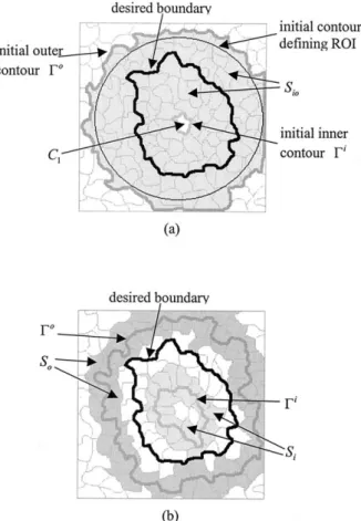
As illustrated in Fig. 3a, the ROI is delineated by a circle and the minimum covering cells are those cells inside the outermost thick gray contour, which is the initial outer contour ⌫o. The central cell within the ROI is assumed to be C1and the thick gray boundary
of C1 is the initial inner contour ⌫ i
. The gray area marks the set of cells enclosed by⌫oand⌫i, which is
Sio. Figure 3b illustrates the outer contour ⌫oand the
inner contour ⌫i for an intermediate step during de-formation; these are indicated by the outermost and
the innermost gray thick contours, respectively. The outer and the inner gray areas define the cells neigh-boring ⌫o and ⌫i, which are S
o and Si, respectively.
The thick black contours in both Figs. 3 and 4 repre-sent the desired boundary.
The energy function of the proposed dual snake (CBDS) model, denoted as ECBDS, is defined as ECBDS⫽
E(⌫i艛 ⌫o)⫽ E(⌫i)⫹ E(⌫o), where E(⌫) stands for the energy of the contour⌫. Both E(⌫i) and E(⌫o) are
com-prised of four energy terms as defined in eqn (3).
E共⌫兲 ⫽␣Elen共⌫兲 ⫹E共⌫兲 ⫹␥Eⵜ共⌫兲
⫹␦EArea共⌫兲 (3)
and Fig. 2. Illustration for the flooding step of the immersion
method for that example given in Fig. 1. The resulting labels and watersheds are shown while the elevation level increases from 1 to 5. As a result, one watershed, “w,” separating two catchment basins, “1” and “2,” respectively, are constructed.
Fig. 3. (a) The ROI is delineated by a circle and the minimum covering cells are those cells inside the outermost thick gray contour, which is the initial outer contour. The boundary of the cell C1 is the initial inner contour. (thick black contour) the
desired boundary; (gray area) Sio. (b) The outermost and the
innermost thick gray contours are the outer contour⌫o
and the inner contour⌫i
for an intermediate step during deformation, respectively. The outer and the inner gray areas indicate Soand
Elen共⌫兲 ⫽
冘
j⫽1 N 兩⌫共 j兲兩 (4) E共⌫兲 ⫽冘
j⫽1 N 共⬔⌫共 j兲兲 (5) Eⵜ共⌫兲 ⫽冘
j⫽1 N 兩ⵜI共j兲兩 (6) EArea共⌫兲 ⫽冘
j⫽1 N Area共Sio兲 (7)where 僆 {i, o}, Ndenotes the numbers of snake ele-ments in⌫, andj⫽ (xj, yj) represents the position of the
jth snake element of⌫. It should be noted that all snake elements in both of the inner and the outer contours partic-ipate in deformation in the proposed dual snake model and, thereby, are involved in computing E(⌫).
The first energy Elenis the length of the two
con-tours, which is the sum of the distance of every two consecutive snake elements. The distance between two consecutive snake elements is denoted by兩⌫(j)兩 in eqn (3). Minimizing this energy would force the inner snake into expanding outward and the outer snake into con-tracting inward, which is achieved by setting␣iand␣oto
a negative and a positive number, respectively. The sec-ond energy, E, is the total sum of the turning angles evaluated at all snake elements. The turning angle of the
jth snake element, which is used to approximate the
curvature, is defined as:
⬔⌫共 j兲 ⫽ cos⫺1
冉
uជj䡠ជj兩uជj兩兩ជj兩
冊
(8)
where 0 ⱕ ⬔⌫共j兲 ⬍ , uជj ⫽ 3j⫺3jandជj ⫽ 3jj⫹3. This
energy is to control the smoothness of the derived bound-ary. If a highly winding contour is expected for the desired boundary, the weighting factors,iando, should be kept
small. The third energy, Eⵜ, is the image energy serving as the major force to latch the snakes at the desired boundary. The image energy used in this study is the intensity of the gradient map, which is denoted as兩ⵜI(j)兩 in eqn (3). Note
that␥should be set to a negative number for the energy minimization purpose. The last energy, EArea, is the area
covered by the cells in Sio. Minimization of this energy
provides the attraction force to pull the inner and the outer snakes to each other. Because these four energies have different dynamic ranges to prevent any energy term from dominating the energy minimization process, the target function to be minimized is the normalized energy variation
⌬ECBDS rather than the ECBDS in each iteration.
Corre-sponding to the four energies defined in the ECBDS, the
⌬ECBDSconsists of four normalized energy variation terms,
as defined in eqn (9).
⌬ECBDS共⌫兲 ⫽␣⌬Elen共⌫兲 ⫹⌬E共⌫兲 ⫹␥⌬Eⵜ共⌫兲
⫹␦⌬EArea共⌫兲 (9) and ⌬E共⌫兲 ⫽关E共⌫new i 兲 ⫹ E共⌫new o 兲兴 ⫺ 关E共⌫current i 兲 ⫹ E共⌫current o 兲兴 关E共⌫current i 兲 ⫹ E 共⌫current o 兲兴 (10) Fig. 4. (a) An illustration of cell-erosion operation using the
inner contour as an example, in which the union of the outer and the inner gray areas illustrates ((Si艛 So)艚 Sio). (b) An
illustration of cell-dilation using the outer contour as an exam-ple, in which the union of the outer and the inner gray areas
where the subscript 僆 {len, , ⵜ, Area}, and the subscripts “current” and “new” stand for the current contour and the new contour, respectively.
Two kernel operators are involved in the cell-based deformation with respect to Sio. One is the cell-erosion
operator, CE(Sio, Cp), which is defined as Sio⫺ {Cp},
where the cell Cp僆 ((Si艛 So)艚 Sio) (i.e., the set of cells
enclosed by and neighboring⌫iand⌫o). Figure 4a illus-trates the cell-erosion operation using the inner contour as an example. The gray areas indicate the set of cells ((Si
艛 So) 艚 Sio) before erosion. During erosion, the inner
contour⌫iincludes the boundary of the cell Cp僆 ((Si艛
So)艚 Sio) and eliminates the contour segment (marked
by two black short sticks) that was previously shared by
⌫i
and the boundary of Cp.
The other kernel operator is the cell-dilation oper-ator, CD(Sio, Cq), which is defined as Sio艛 {Cq}, where
the cell Cq僆 ((Si艛 So)\Sio) and (Si艛 So)\Siois the set
of cells neighboring ⌫i and⌫o, and outside Sio. Taking
the outer contour as an example, the cell-dilation opera-tion is demonstrated in Fig. 4b. The gray areas mark the set of cells (Si艛 So)\Siobefore dilation. During dilation,
the outer contour ⌫oconcatenates the boundary of the cell Cq僆 ((Si 艛 So)\Sio) and removes the contour
seg-ment (marked by seven black short sticks) that was previously shared by⌫oand the boundary of Cq.
The cell-based deformation is a series of greedy cell-erosion and cell-dilation operations to minimize
⌬ECBDS. The deformation starts with the initial inner and
outer contours and continues until Siobecomes an empty
set (i.e., when both⌫i and⌫omeet each other). In each iteration, both cell-erosion and cell-dilation operations will be evaluated, but only the one rendering the minimal
⌬ECBDSwill be carried out. The cell-based deformation
algorithm may be sketched as follows: 1. Initialization
Given the minimum covering cells, C1, C2, . . . ,Ck,
that contain the ROI R and assuming that the center of the ROI is in C1. Sio⫽ 艛j⫽2 k 兵C j其, ⌫ i⫽ ⌿共S io兲, ⌫ o⫽ ⌽共S io兲 (11) 2. While Sio ⫽ Ce⫽ arg min Cj⑀共共Si艛So兲艚Sio兲 兵⌬E共⌿共CE共Sio,Cj兲兲 艛 ⌽共CE共Sio,Cj兲兲兲其 (12) Cd⫽ arg min Cj⑀共共Si艛So兲\艚Sio兲 兵⌬E共⌿共CD共Sio,Cj兲兲 艛 ⌽共CD共Sio,Cj兲兲兲其 (13)
⌬Eerode⫽ ⌬E共⌿共CE共Sio, Ce兲兲 艛 ⌽共CE共Sio, Ce兲兲兲 (14)
⌬Edilate⫽ ⌬E共⌿共CD共Sio, Cd兲兲
艛 ⌽共CD共Sio, Cd兲兲兲 (15)
If ⌬Eerode ⱕ ⌬Edilate, then Sio ⫽ CE(Sio, Ce).
Else Sio⫽ CD(Sio, Cd)
⌫i⫽ ⌿共S
io兲, ⌫o⫽ ⌽共Sio兲 (16)
Contour smoothing
Contour smoothing is an optional process to smooth the boundary derived by the cell-based deformation. Because of the speckle and the tissue-related textures, this boundary usually has a zigzag nature. Two possible approaches may be employed for contour smoothing. One approach is using a conventional deformable model (e.g., the Kass’s snake model). It is feasible because the derived boundary has been very close to the desired boundary. The other approach is using the spline inter-polation. When the boundary of the object of interest has a reasonably strong edge, the conventional deformable model is preferred to the spline interpolation. The reason is that the spline interpolation incorporates no notion of the boundary definition, whereas the conventional de-formable model may take advantage of the gradient to catch the boundary more accurately. On the contrary, if some portions of the desired boundary have weak edges, using a conventional deformable model may make the final derived boundary seriously deviate from the desired boundary, especially when these portions have high cur-vatures. Taking into account the high-curvature feature of the malignant lesions in the US images used for performance evaluation, in this paper, we present the contour smoothing results derived by using the spline interpolation. One may refer to Huang (2001) for the results derived by using the conventional deformable model for contour smoothing.
Images for performance analysis
To evaluate the performance of the proposed cell-based dual snake model quantitatively, synthetic images with simulated speckle and undesirable structures are used in this study. Because the desired boundary of the synthetic image is known in advance, the quantitative comparison between the desired boundary and the de-rived boundary of the synthetic image serves as the exact performance evaluation. The raw synthetic image with sporadic undesirables used in this study is given in Fig. 5a, in which the central circular disk is the object of interest. The size of the raw synthetic image is 256⫻ 256 and the radius and the center of the disk are 32 and (128, 128), respectively. The desired boundary of the object of interest is shown in Fig. 5b.
To simulate the speckle in a displayed US image, the raw synthetic image is corrupted by the log-com-pressed fully developed speckle generated by using the speckle-simulation method reported in Li and O’Donnell (1994). The specifications of the simulated scanner are listed below:
1. Scanner type: 128-element linear array, 2. Interelement space: 0.25 mm,
3. Central frequency/bandwidth: 3 MHz/1 MHz. It is assumed that the shape of the envelope of the axial response is Gaussian and the point spread function of the scanner is spatially invariant. The lateral response is the Fourier transform of the aperture function. As an example, Fig. 6a demonstrates a synthetic image with simulated speckle, the contrast-to-noise ratio (CNR) of which is about 2. The CNR is defined as:
CNR⫽ 兩gf⫺ gb兩
max共f,b兲
, (17)
fandbare the SD of the speckle within and outside the
disk, excluding the undesirables, and gf and gbare the
grey levels of the disk and the background.
In addition to the synthetic images, the performance of the proposed cell-based dual snake model is also evaluated on the clinical US images, which offer the realistic complex image condition for performance eval-uation. Unlike the synthetic images for which the desired boundaries are predefined, the desired boundaries for clinical US images are manually demarcated by experi-enced medical doctors. Because the delineated boundary may be different for different medical doctors, or even for the same medical doctor at different times, the anal-ysis results on the clinical US images are better regarded as a reference rather than as an exact evaluation.
A total of 16 US images, including 6 liver and 10 breast US images, were used in this study, each of which contained a lesion. All these 16 images were captured
from the RGB outputs of a Toshiba SSA-380A clinical US imaging system by using a frame-grabber card. The frame-grabber card, Meteor-II card, is made by the Ma-trox Electronic System Ltd., (Dorval, Quebec, Canada). The operating frequency of the scanner was 3 MHz. The image format was Windows BMP format with 8-bit resolution for each color channel. These 16 images were carefully selected to account for the winding property of the boundary, the undesirable structures, the hyperechoic and hypoechoic natures of the lesions. For example, two hepatic tumors are shown in Fig. 7a and b, and two breast lesions are given in Fig. 7c and d. The boundaries of Fig. 5. (a) The raw synthetic image, including the object of
interest (i.e., the circular disk and sporadic undesirables); (b) the desired boundary of the object of interest.
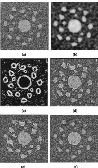
Fig. 6. (a) A synthetic image with simulated speckle, the CNR of which is about 3; (b) despeckled image derived by using 10-level Gaussian filters; (c) gradient map obtained by applying the Sobel edge detector to the despeckled image; (d) cells generated by two-pass watershed transform; (e) initial contour, indicated by the big white circle, and the cells covering the ROI enclosed by the initial contour; (f) the boundary derived by using the cell-based
these four lesions are marked by the white contours. The hepatic tumor in Fig. 7a is hyperechoic and the other three lesions in Fig. 7b and c are hypoechoic. Undesir-ables can be generally found in the vicinity of these four lesions. The breast lesion in Fig. 7c has a highly winding contour and that in Fig. 7d has weak edges around the upper-right corner of the lesion.
Let⌫CBDSand⌫* denote the derived boundary and the
desired boundary, respectively. The derived boundary is evaluated in terms of the mean, the SD, and the maximum of the minimal distances from the derived boundary points to the desired boundary. The procedure to compute these three parameters is described as follows.
1. For each pi ⑀ ⌫CBDS, find p*i ⑀ ⌫* so that p*i ⫽ arg
min@p*
j僆⌫* 储pi ⫺ p*j储, where 储a ⫺ b储 means the
Eu-clidean distance between pixels a and b.
2. For all (pi, p*i), compute the Euclidean distance, derror i
⫽ 储pi ⫺ p*i储.
3. Find the mean, SD and maximum of {derror
i 兩 @p
i 僆
⌫CBDS}.
IMPLEMENTATION RESULTS AND DISCUSSION
The exact performance evaluation of the proposed cell-based dual snake model was carried out by using the
synthetic images with 10 different CNRs, which include
CNR⫽ {0.5, 1, 2, 3, 4, 5, 6, 7, 8, 9}. The same initial
contour has been used for these 10 synthetic images to ensure the same initial condition. For those synthetic images with CNR ⱖ 5, the number of levels for the multiscale Gaussian filtering is set to 5. When CNR⬍ 5, the number of levels is set to 10 to provide a larger-scale smoothing effect. The SD for the ith-level Gaussian filter is set to i, where i⫽ {1, 2, . . . , 10}, and the size of the Gaussian filter is 13⫻ 13.
Take the synthetic image with CNR ⫽ 3 as an example, which is shown in Fig. 6a. Figure 6b shows the speckle-reduced image by using the 10-level Gaussian filtering. Figure 6c presents the gradient map attained by using the Sobel edge detector. Although the multiscale Gaussian filtering has significantly reduced the speckle, the false edges caused by the remaining noise and unsirable structures may still prevent the conventional de-formable models from having a distant initial contour.
Figure 6d demonstrates the cells derived by using the two-pass watershed transform. One may see that the object of interest is well-covered by a number of cells, which forms the basis of the cell-based defor-mation. Note that the entire image itself is considered to be a giant cell. The initial contour defining the ROI for the cell-based deformation is given in Fig. 6e as a big white circle. The cells shown in Fig. 6e, which are delineated with the white contours, cover the ROI enclosed by the initial contour. Figure 6f shows the boundary derived by the cell-based deformation. As expected, the derived boundary is zigzag and requires further smoothing. The final boundary derived after contour smoothing by using the spline interpolation is given in Fig. 8b, which is clearly smoother than the boundary shown in Fig. 6f.
The overall performance of the proposed cell-based dual snake model for the 10 synthetic images is summa-rized in Fig. 9, in which the labels “Mean,” “Max” and “Std” stand for the mean, the maximum, and the SD of the minimal distances from the derived boundary points to the desired boundary, respectively. The performance plot clearly indicates that the proposed cell-based dual snake model is robust in the sense that, as CNRⱖ 1, the mean minimal distance is less than 1. Moreover, most derived boundary points are within 1.8 pixels (“Mean”⫹ “Std”) from the desired boundary points and the maximal discrepancy between the derived boundary and the de-sired boundary seems to be stabilized as CNRⱖ 3.
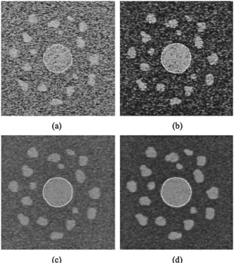
To visually evaluate the final results attained by the proposed cell-based dual snake model, Fig. 8a– d pro-vides the final boundaries for the cases of CNR⫽ {1, 3, 5, 7}. Even though distant initial contours have been used for all cases, the derived boundaries coincide with the desired boundaries reasonably well, in general, tak-Fig. 7. (a) A hyperechoic hepatic tumor; (b) hypoechoic hepatic
tumor; (c) hypoechoic breast lesion with a highly winding contour; and (d) hypoechoic breast lesion with weak edges. The boundaries of these four lesions are marked manually by the
ing into account the various CNRs. The mean minimal distances for these four cases (i.e., CNR⫽ {1, 3, 5, 7} are 1.0, 0.8, 0.7 and 0.7 pixels, respectively. The discrepancy between the derived boundary and the desired boundary may be mainly ascribed to the despeck-ling process, which inevitably distorts the edge of the object of interest. This phenomenon becomes more evi-dent as CNR gets smaller. It is expected that the
perfor-mance of the cell-based dual snake model may be further improved if a better speckle-reduction algorithm is em-ployed.
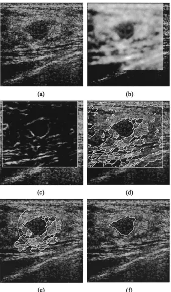
Promising results have also been obtained for clinical US images. The initial contour defining the ROI for each US image is given as a circle containing the object of interest. Suppose the radius of the circle is r. Then, all computations involved in the proposed cell-based dual snake model have been confined within the 2r⫻ 2r square centered at the center of the circular ROI. As an example, Fig. 10 presents the intermediate results of the proposed cell-based dual snake model for one of the 16 tested US images. Figure 10a is a clip of a breast sonography with a benign lesion. The manually delineated boundary of this lesion is given in Fig. 7d. Figure 10b shows the despeckled image by using the 10-level Gaussian fil-tering. The circular ROI with a radius of r is illustrated in Fig. 10e, which is marked as a white circle. Note that only the 2r⫻ 2r square centered at the center of the circular ROI has been despeckled. Figure 10c gives the gradient map computed by using the Sobel edge detector. It can be seen that, even after the speckle has been largely removed, the lesion is still surrounded by the significant edge of the undesirable structures, which result in the cells in the vicinity of the lesion as shown in Fig. 10d. Figure 10e displays the cells covering the ROI, the boundary of which is indicated by the white circle. The lesion boundaries derived at the end of the cell-based deformation and the contour smoothing stages are provided in Figs. 10f and 11d, respectively.
As a reference, the performances of the proposed cell-based dual snake model on these 16 US images are plotted in Fig. 12, which reports the same three statistics (i.e., “Mean,” “Max” and “Std,” as defined in Fig. 9). Generally speaking, the proposed algorithm has achieved reasonably good performances for clinical US images. Most derived boundary points are within three pixels from the desired boundary points. Furthermore, as for the synthetic images, the proposed algorithm exhibits reli-able performance for clinical US images in that the mean and the SD of the minimal distances between the derived and the desired boundaries are similar for all tested cases. Figure 11 presents the boundaries derived after contour smoothing for the four clinical US images shown in Fig. 7. The mean minimal distances for these four clinical US images (i.e., Fig. 11a– d, are 1.2, 1.0, 0.9 and 1.7 pixels, respectively). One can see that the derived boundaries are visually acceptable and have reasonably delineated the object of interest. Based on Figs. 11 and 12, we may conclude that the proposed cell-based dual snake model has successfully penetrated the interference of the speckle and the undesirable structures and, thus, allows a Fig. 8. The final boundaries derived after contour smoothing for
the synthetic images with (a) CNR⫽ 1; (b) CNR ⫽ 3; (c) CNR ⫽ 5; (d) CNR ⫽ 7.
Fig. 9. The overall performance of the proposed cell-based dual snake model for the 10 synthetic images, in which the labels “Mean,” “Max” and “Std” stand for the mean, the maximum, and the SD of the minimal distances from the derived boundary
distant initial contour. Figure 11c further suggests that the proposed algorithm is capable of capturing the highly winding contour, which is not easily achieved by most conventional deformable models.
The discrepancy between the derived and the de-sired boundaries may be imputed to three factors. As observed for the synthetic images, the first factor is the distortion effect caused by the speckle-reduction pro-cess on the edge definition of the object of interest. This distortion effect may be more serious on a clin-ical US image than on a synthetic image, for the former usually has a lower CNR than the latter. The
second factor is that the boundary defined by a medical doctor may be somewhat different from that defined by the gradient. Moreover, boundary delineation is quite a subjective process, so that diverse boundary definitions may be given by different medical doctors, due to different medical knowledge and experience. The third factor is the weak edges or missing edges frequently found in the boundaries of the object of
Fig. 10. (a) A clip of breast US image with a benign lesion; (b) despeckled image obtained by using 10-level Gaussian filters; (c) gradient map attained by using the Sobel edge detector; (d) cells produced by the two-pass watershed transform; (e) initial contour marked by the big white circle and the cells covering the ROI; (f) boundary derived by using the cell-based
defor-mation, which is marked by the white contour.
Fig. 11. The final boundaries derived after contour smoothing for the four US images given in Fig. 7.
Fig. 12. The overall performance of the proposed cell-based dual snake model for the 16 clinical US images, in which the first 10 images are the breast US images and the last 6 images are the liver US images. The labels “Mean,” “Max” and “Std” denote the mean, the maximum and the SD of the minimal distances from the derived boundary points to the desired
interest, which may lead to quite different boundary definitions given by the medical doctors and the im-age-processing techniques. For example, the contour around the upper-right corner of the lesion boundary in Fig. 11d is different from that delineated by the medical doctor, as shown in Fig. 7d. Although there does exist a cell in the upper-right corner of the lesion boundary, as shown in Fig. 10d, the cell edge is too weak to be adopted in the final derived boundary.
CONCLUSIONS
A new deformable model for sonographic bound-ary detection, namely, the cell-based dual snake model, is proposed in this paper. The proposed de-formable model aims to allow a distant initial contour and to capture the highly winding contours of the objects of interest in the US images. The principal idea of the proposed cell-based dual snake model is to guide two snakes, one inside and the other outside of the object of interest, toward each other in the cell-based deformation manner. The dual-snake model pro-vides an effective mechanism to allow a distant initial contour, whereas the cell-based deformation makes it possible to catch the winding characteristics of the desired boundary. The discrete concept inherent in the cell-based deformation promises that the derived boundary is right on the edge points defined by the watersheds, which are determined by the watershed transform with the immersion method.
The performance of the proposed cell-based dual snake model has been evaluated on two types of images. One is the synthetic image with simulated speckle and undesirable structures, and the other is the clinical US image. All initial contours have been set to be reasonably far away from the desired boundaries. The experimental results show that the proposed cell-based dual snake model is robust, in the sense that the mean and the SD of the minimal mean distance from the derived boundary points to the desired boundary points are similar for most tested cases in each type of image. Moreover, most derived boundary points are within 1.8 pixels and 3.0 pixels from the desired boundary points for the synthetic and the clinical US images, respectively.
REFERENCES
Akgul YS, Kambhamettu C, Stone M. Automatic extraction and track-ing of the tongue contours. IEEE Trans Med Imagtrack-ing 1999;18: 1035–1045.
Boukerroui D, Basset O, Guerin N, Baskurt A. Multiresolution texture based adaptive clustering algorithm for breast lesion segmentation. Eur J Ultrasound 1998;8:135–144.
Chalana V, Linker DT, Haynor DR, Kim Y. A multiple active contour model for cardiac boundary detection on echocardiographic se-quences. IEEE Trans Med Imaging 1996;15:290–298.
Chen CM, Lu HHS, Lin YC. An early vision based snake model for ultrasound image segmentation. Ultrasound Med Biol 2000;26(2): 273–285.
Cohen LD, Cohen I. Finite-element methods for active contour models and balloons for 2-D and 3-D images. IEEE Trans Pattern Anal Machine Intel 1993;15:1131–1147.
Fan L, Braden GA, Herrington DM. Nonlinear wavelet filter for intra-coronary ultrasound images. Proceedings of the 1996 23rd Annual Meeting on Computers in Cardiology, 1996:41– 44.
Gauch JM. Image segmentation and analysis via multiscale gradient watershed hierarchies. IEEE Trans Image Processing 1999;8(1):69– 79.
Giraldi GA, Goncalves LM, Oliveira AAF. Dual topologically adapt-able snakes. Proceedings of the 5th Joint Conference on Informa-tion Science. 2000;2:103–106.
Gunn SR, Nixon MS. A robust snake implementation: A dual active contour. IEEE Trans PAMI 1997;19:63–68.
Haas C, Ermert H, Holt S, et al. Segmentation of 3-D intravascular ultrasonic images based on a random field model. Ultrasound Med Biol 2000;26:297–306.
Hafner E, Schuchter K, Van Leeuwen M, et al. Three-dimensional sonographic volumetry of the placenta and the fetus between weeks 15 and 17 of gestation. Ultrasound Obstet Gynecol 2001;18:116– 120.
Hamdan HM, Youssef AB, Rasmy ME. The potential of mathematical morphology for contour extraction from ultrasound images. Pro-ceedings of the 18th Annual International Conference of the IEEE EMBS 1996;881– 882.
Haris K, Efstratiadis SN, Maglaveras N, Katsaggelos AK. Hybrid image segmentation using watersheds and fast region merging. IEEE Trans Image Processing 1998;7(12):1684–1699.
Heckman T. Searching for contours. Proc SPIE 1996;2666:223–232. Huang YH. A cell-based dual snake model for lesion boundary
detec-tion in ultrasound images. MA thesis. Nadetec-tional Chiao-Tung Uni-versity, Hsin-Chu, Taiwan, 2001.
Iwase M. 3-D Echocardiography and semi-automatic border detection to assess left ventricle volume and function: Comparison with MRI. Circulation 1994;90:1337.
Kass M, Witkin A, Terzoulos D. Snake: Actour contour models. Int J Comput Vision 1987;1:321–331.
Kerschner M. Homologous twin snakes integrated in a bundle block adjustment. Proceedings of Symposium on Object Recognition and Scene Classification from Multispectral and Multisensor Pixels, 1998 (http://www.ipf.tuwien.ac.at/veroeffentlichungen/mk_p_isprs98/ paper3.htm).
Kotropoulos C. Nonlinear ultrasonic image processing based on signal-adaptive filters and self-organizing neural networks. IEEE Trans Image Processing 1994;3:65–77.
Lefebvre F, Berger G, Laugier P. Automatic detection of the boundary of the calcaneous from ultrasound parametric images using an active contour model: Clinical assessment. IEEE Trans Med Imag-ing 1998;17:45–52.
Li PC, O’Donnell M. Improved detectability with blocked element compensation. Ultrason Imaging 1994;16:1–18.
Mikic I, Krucinski S, Thomas JD. Segmentation and tracking in echo-cardiographic sequences: Active contours guided by optical flow estimates. IEEE Trans Med Imaging 1998;17:274–284.
Pathak SD, Chalana V, Kim Y. Interactive automatic fetal head mea-surements from ultrasound images using multimedia computer technology. Ultrasound Med Biol 1997;23:665–673.
Sarty GE, Liang W, Sonka M, Pierson RA. Semiautomated segmenta-tion of ovarian follicular ultrasound images using a knowledge-based algorithm. Ultrasound Med Biol 1998;24:27–42.
Shekhar R, Cothren RM, Vince DG, et al. Three-dimensional segmen-tation of luminal and adventitial borders in serial intravascular ultrasound images. Comput Med Imaging Graphics 1999;23:299– 309.
Skaane P, Engedal K. Analysis of sonographic features in the differ-entiation of fibroadenoma and invasive ductal carcinoma. AJR 1998;170:109–114.
Solaiman B, Roux C, Rangayyan RM, Pipelier F, Hillion A. Fuzzy edge evaluation in ultrasound endosonographic images. Proceed-ings of the 1996 Canadian Conference on Electrical and Computer Engineering, 1996:335–338.
Stavros AT, Thickman D, Rapp CL, et al. Solid breast nodules: Use of sonography to distinguish between benign and malignant lesions. Radiology 1995;196:123–134.
Terzopoulos D, Witkin A, Kass M. Constraints on deformable models: Recovering 3D shape and nonrigid motion. Artif Intell 1988;36: 91–123.
Thomas JG, Peters RA, Jeanty P. Automatic segmentation of ultra-sound images using morphological operators. IEEE Trans Med Imaging 1991;10:180–186.
Vincent L, Soille P. Watershed in digital spaces: An efficient algorithm based on immersion simulations. IEEE Trans PAMI 1991;13(6): 583–597.
Wang D. A multiscale gradient algorithm for image segmentation using watersheds. Pattern Recognition 1997;30(12):2043–2052. Xu C, Prince JL. Snakes, shapes, and gradient vector flow. IEEE Trans
Image Processing 1998;7:359–369.
Zimmer Y, Tepper R, Akselrod S. A two-dimensional extension of minimum cross entropy thresholding for the segmentation of ultra-sound images. Ultraultra-sound Med Biol 1996;22:1183–1190.