Abstract—This paper argues that increased uncertainty, in certain situations, may actually encourage investment. Since earlier studies mostly base their arguments on the assumption of geometric Brownian motion, the study extends the assumption to alternative stochastic processes, such as mixed diffusion-jump, mean-reverting process, and jump amplitude process. A general approach of Monte Carlo simulation is developed to derive optimal investment trigger for the situation that the closed-form solution could not be readily obtained under the assumption of alternative process. The main finding is that the overall effect of uncertainty on investment is interpreted by the probability of investing, and the relationship appears to be an invested U-shaped curve between uncertainty and investment. The implication is that uncertainty does not always discourage investment even under several sources of uncertainty. Furthermore, high-risk projects are not always dominated by low-risk projects because the high-risk projects may have a positive realization effect on encouraging investment.
Keywords—real options, geometric Brownian motion, mixed diffusion-jump process, mean- reverting process, jump amplitude process
I. INTRODUCTION
HE relationship between uncertainty and investment has
fascinated financial economists for a long time. Early literature on real options theory argues that increased uncertainty causes a decrease in the current level of investment by raising the value of option of waiting. For example, Cukierman [3] presents a Bayesian framework to address the idea that an investment opportunity can be more valuable by waiting longer for more information arrivals. Pindyck [12, 13] and Dixit [4, 5] also find that a higher level of uncertainty not only increases option value, but also brings about a higher optimal investment trigger to such an extent that uncertainty may in effect discourage investment.
Some studies based on real options theory suggest that the relationship between uncertainty and investment is non-monotonic. [6] Abel and Eberly [1] further contend that the uncertainty-investment relationship is positive for a lower of uncertainty while the relationship is negative for a high level of uncertainty, suggesting an inverted U-shaped relationship.
Extending standard real options theory, Sarkar [15] and Rhys, Song, and Jindrichovska [14] explore the relationship between uncertainty and investment by asking the question how much the likelihood is that a project value, V, would reach optimal investment trigger, V*, given that the project value evolves as a geometric Brownian motion (GBM). Both studies
apply a similar probability function, and find that the uncertainty-investment relationship is not always negative. They show that increased uncertainty under a GBM, in certain situations, may encourage investment due to a higher probability of investing or an earlier time of first passage.
Recent studies on investment theory suggest that the relationship between uncertainty and investment mostly is nonlinear. Lensink and Murinde [7] empirically examine the data of UK firms and propose the inverted-U hypothesis for the effect of uncertainty on investment. In addition, Wong [18] analyzes optimal investment timing in a real options model and argues that optimal investment trigger exhibits a U-shaped pattern against project volatility.
This paper aims to investigate the uncertainty-investment relationship by relaxing the assumption of state variable to various stochastic processes by applying the technique of Monte Carlo simulation. The stochastic of interest are GBM, mixed diffusion-jump (MX), mean-reverting process (MR), and jump amplitude process (JA). Earlier studies, such as Sarkar [15] and Rhys et al. [14], apply a probability function to measure the probability of reaching a critical value under a GBM, yet their models fail to address the relationship between uncertainty and investment under an alternative stochastic process. In contrast, Monte Carlo simulation is relatively flexible and advantageous when the underlying variable follows an alternative process in a finite time horizon.
The rest of the paper is organized as follows: Section 2 introduces the specifications of alternative stochastic processes both in continuous time and in discrete time, serving as a foundation for the subsequent sections. Section 3 proposes the approach of Monte Carlo simulation for deriving optimal investment trigger in a more general setting. Section 4 examines the relationship between uncertainty and investment by decomposing the overall effect into the effect of uncertainty and the effect of realization. The probability of investing is then suggested to measure the overall effect of uncertainty on investment. Section 5 gives concluding remarks.
II. OPTIMAL INVESTMENT TRIGGER
Since volatility component in stochastic process is regarded as major source of uncertainty in evaluating capital investments, in this section a variety of stochastic processes are introduced as well as the derivation of optimal investment triggers.A framework of Monte Carlo simulation for deriving optimal investment is also proposed for alternative stochastic models that could not be readily solved for a closed form solution.
George Yungchih Wang
National Kaohsiung University of Applied Science, Taiwan
A Framework of Monte Carlo Simulation for
Examining the Uncertainty-Investment
Relationship
T
A. Geometric Brownian Motion
In traditional real options literature, the GBM assumption is widely assumed to address for the uncertainty of random walk. The main property of GBM is that the rate of return is assumed to be normally distributed, implying a lognormal distribution of the project value. A GBM in continuous time is expressed as follows:
dV=αVdt+σVdz (1) where α , σ , and dz denote drift rate, instantaneous volatility, and an increment of a standard Wiener process, respectively.
A GBM process in discrete time could be changed into the following form:
lnV v t σ tε
Δ = Δ + Δ (2) where
Δ
t
andε
represent a small interval of time and a random drawing from a standard normal distribution, respectively, and v=α -σ 2/2.Suppose a firm is presented with an investment opportunity that pays an irreversible investment cost, I, in return for an uncertain project value, V. This is a standard problem of optimal investment timing in real options literature. V is considered to be the major source of uncertainty and is normally assumed to follow a GBM as in Equation (1) due to the ease of deriving a tractable solution. The value of an investment opportunity is determined by an optimal investment policy that maximizes the option value. Let F(V) denote the value of the investment opportunity and the superscript * denote optimality. McDonald and Siegel [8], Pindyck [13], and Dixit and Pindyck [6] have demonstrated that the optimal investment trigger is given by
1 1 1 GBM b V I b ∗ = ⎜⎛ ⎞ ⎟ − ⎝ ⎠ (3) where VGBM
∗ and I denote the optimal GBM trigger and the
investment cost, respectively, and
2 1 2 2 2 1 1 2 2 2 r r r b δ δ σ σ σ − − ⎛ ⎞ ⎛ ⎞ =⎜ − ⎟+ ⎜ − ⎟ + ⎝ ⎠ ⎝ ⎠ (4)
where δ represents convenience yield of holding a project, which also implies the opportunity cost of deferring a project. B. Mixed Diffusion-Jump Process
While the preceding GBM could describe the incremental changes of random walk, the process fails to capture the significant impact of random informational arrival. A mixed diffusion-jump process thus is proposed to combine a Poisson jump process into a GBM, expressed as follows:
( ) 1
dV= α λ− k Vdt+σVdz Vdq+ (5)
where dq1 is an increment of a Poisson jump process with a mean arrival rate
λ
such that1 with a probability of 0 with a probability of 1-dt dq dt ϕ λ λ ⎧ = ⎨ ⎩ (6)
where φ ~N(k, σφ) denotes a proportional jump relative to V
if a jump occurs.
Note that the Poisson jump term dq1 is assumed to be independent of dz such that E(dq1dz)=0. Equation (6) also reveals that the actual growth rate of such a mixed diffusion-jump process is not α but instead (α -λ k) in order to adjust the influence of a Poisson event. For the simulation purpose, the discrete-time version of the mixed diffusion-jump process is given as follows:
1
lnV v t σ tε D
Δ = Δ + Δ + (7) where D1 denotes an increment of a Poisson jump in discrete time with a mean arrival rate λ such that
1 with a probability of 0 with a probability of 1-t D t ϕ λ λ Δ ⎧ = ⎨ Δ ⎩ (8)
It is worth noting that McDonald and Siegel (1986) and Dixit and Pindyck (1994) also propose a mixed diffusion-jump process with the sign of the jump term changed into negative to describe the situation in that the project becomes suddenly worthless when a major competitor of the same product enters the market.
For an investment opportunity whose value follows a mixed diffusion-jump process, McDonald and Siegel [8] and Dixit and Pindyck [6] show that when the value of the project may be appropriated by competitive arrivals such that the project becomes suddenly worthless, the solution of optimal trigger under such a mixed diffusion-jump process, V*
MX, has the same form as Equation (3) with b1 substituted by b2 as follows:
2 2 2 2 2 1 1 2( ) 2 2 r r r b δ δ λ σ σ σ − − + ⎛ ⎞ ⎛ ⎞ =⎜ − ⎟+ ⎜ − ⎟ + ⎝ ⎠ ⎝ ⎠ (9)
where λ denotes the jump intensity of competitive arrivals. C. Mean-Reverting Process
Another class of commonly used stochastic process is a mean-reverting process which is often proposed to describe the price behavior of commodity and natural resources. The most prominent property of a mean-reverting process is that its growth rate is not a constant but instead a function of a difference between current value and long-run mean, suggesting that growth rate in effect responds to disequilibrium. Dixit and Pindyck [6] examine the value of an investment opportunity whose value follows a mean-reverting process. The specification of this commonly used mean-reverting process is given below:
(
)
dV=η V−V Vdt+σVdz (10) where η denotes a speed of mean reversion and V is a
long-run mean.
As there are many ways to specify a mean-reverting process, Dixit and Pindyck’s specification is somewhat arbitrary but convenient to find a “quasi-analytical” solution for the value of the project. Equation (10) can be alternatively expressed into the following equation in discrete time:
(
)
1 2 ln 2 V ⎡η V V σ ⎤ t σ tε Δ =⎢ − − ⎥Δ + Δ ⎣ ⎦ (11)Under the assumption of a mean-reverting process, Dixit and Pindyck [6] provide the solutions of an investment opportunity and optimal investment trigger, respectively, as follows: ( ) ( ) ; , F V =BV G xθ θ g (12)
( )
MR MR V∗ =F V∗ +I (13) where 2 2 2 2 1 1 2 2 2 V V r η η θ σ σ σ ⎡ ⎤ = − + ⎢ − ⎥ + ⎣ ⎦ , 2 2 x ηV σ = , 2 2 2 V g θ η σ = + , and ( ; , ) 1 ( 1) 2 ( 1)( 2) 3 ( 1) 2! ( 1)( 2) 3! x x G x g x g g g g g g θ θ θ θ θ θ θ = + + + + + + + + + + L.Note that G(x, θ ,g) stands for an infinite confluent hypergeometric function, and thus the value of the investment opportunity cannot be readily solved. Both Equation (12) and (13) must be solved numerically from an iterative procedure to obtain V* and F(V*).
D. Jump Amplitude Process
To capture the major impact of technological breakthrough and informational arrivals in an R&D project, Pennings and Lint [11] suggest a jump amplitude process to evaluate such an investment opportunity. The jump amplitude process differs from other types of jump process in a sense that it allows for a random jump direction and a stochastic jump size in order to characterize the nature of R&D investments. A jump amplitude process can be mathematically expressed as follows:
2
dV=αVdt Vdq+ (14) where dq2 an increment of a stochastic jump process. The jump term, dq2, is characterized by a parameter of jump intensity λ such that 2 with a probability of 0 with a probability of 1-dt dq dt ϕ λ λ ⎧ = ⎨ ⎩ (15)
where φ denotes a proportional jump relative to V.
By definition, φ =XΓ where X=1 or -1, P(X=1)=p, and Γ
|X~Wei(γ X,2). The jump amplitude process in discrete time is modeled as follows:
2
lnV v t D
Δ = Δ + (16) where D2 denotes an increment of a stochastic jump component in discrete time with a mean arrival rate λ , and D2 is expressed by 2 with a probability of 0 with a probability of 1-t D t ϕ λ λ Δ ⎧ = ⎨ Δ ⎩ (17)
Since there is no closed-form solution for an investment opportunity whose uncertainty evolves as a jump amplitude process. Numerical techniques must be applied to solve both F(V*) and V*.
III. THE FRAMEWORK OF MONTE CARLO SIMULATION
A. The Basic Approach
Since irreversibility complicates capital investments in that closed-form expressions for optimal investment triggers seldom exist under an alternative process, in this section an investment framework for deriving optimal trigger under an alternative process in a finite time horizon is proposed. As it is known that a firm can either defer the project in the unfavorable market condition or launch the project in the favorable market condition, an investment opportunity is equivalent to a call option. Suppose that the investment opportunity will disappear at a finite future time T, if the firm does not take any actions. Therefore, the value of an investment opportunity at time T, given the information set ψT, is expressed as follows:
( ) max( , 0)
T T T T
F V = V −I φ (18) According to Equation (18), the value of investment opportunity at time t can be given by
(T t) max( , 0)
P
t T
F=E ⎡⎣e− − ρ V −I ⎤⎦ (19) where EP denotes an expectation operator in a risk-adjusted world, P a risk-adjusted probability measure, and ρ a risk-adjusted discount rate.
In the risk-neutral world, Ft can be derived from
(T t r) max( , 0) Q t T F=E ⎡⎣e− − V −I ⎤⎦ (20) or (T t r) Q max( ,0) t T F=e− − E ⎡⎣ V −I ⎤⎦ (21) where r denotes a risk-free rate and Q a risk-neutral probability measure.
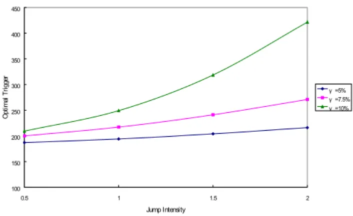
100 150 200 250 300 350 400 450 0.5 1 1.5 2 Jump Intensity Op tim al T rig ge r γ =5% γ =7.5% γ =10% Note: 0 100, 8%, 4%, 1/ 52, 5, 10, 000 V = =I r= δ= Δ =t T= Number of Trials= Fig. 8. The Jump Effect under a Jump Amplitude Process
5% 8% 10%Lambda=0.5 1 1.5 2 0.00% 1.00% 2.00% 3.00% Probability of Investing Jump Size (γ) Jump Intensity (λ) Note: 0 100, 8%, 1/ 52, 4%, 5, 10, 000 V = =I r= Δ =t δ= T= Number of Trials= Fig. 9. The Probability of Investing under a Jump Amplitude Process
as a Function of Jump Intensity (λ) and Jump Size (γ)
As both jump size and jump intensity increase, the jump effect on raising V*
JA becomes more obvious due to an increase in option value, hence leading to a convex, increasing function of both jump intensity and jump size.
To further examine the realization effect, Monte Carlo simulation is conducted to evaluate the probability of investing. Figure 9 presents the sensitivity of the probability of investing to the changes in jump intensity for three different levels of jump size. As seen from Figure 9, the probability of investing appears to be a invested U-shaped curve as jump intensity increases. The probability of investing indicates an increasing function of jump intensity at a lower level of jump intensity, but after a certain point of jump intensity, the probability of investing becomes a decreasing function of jump intensity.
Figure 9 also shows that the curve of the probability of investing climbs up as jump size increases. Since jump size indicates another form of uncertainty, this means that increased uncertainty may increase the probability of investing. As a result, the overall effect of combining jump size and jump intensity does not necessarily discourage investment under a JA process.
V. CONCLUDING REMARKS
Conventional belief in a negative relationship between uncertainty and investment has dominated investment theory for a long time. This paper postulates an argument that increased uncertainty, in certain situations, may actually encourage investment. Since earlier studies mostly base their arguments on the GBM assumption, the study extends the assumption to alternative stochastic processes, e.g., MX, MR, and JA processes, and finds that increased uncertainty in terms of different sources may encourage investment. The overall effect of uncertainty on investment is interpreted by the probability of investing, and found to be an invested U-shaped relationship between uncertainty and investment. This finding is consistent with the conclusion in Lensink and Murinde [7], in which the UK evidence is examined.
The study proposes the technique of Monte Carlo simulation to derive optimal investment trigger and the probability of investing. The overall effect of uncertainty on investment is analyzed by decomposing the overall effect into the variance effect and the realization effect. The former describes the effect that increased uncertainty raises optimal investment trigger, thus discouraging investment; while the latter states that increased uncertainty may in reality increase the probability of investing, thus encouraging investment. For other stochastic processes, additional source of uncertainty is also explored as it may complicate the overall effect on investment. There are several additional effects under alternative processes. First, it is demonstrated that the jump effect under a MX process may lower optimal investment trigger, thus leading to a positive impact on investment. Second, the effect of mean reversion under a MR process may lower optimal investment trigger, thus leading to a positive impact on investment. Third, the effect of stochastic jumps under a JA process are complicated by jump intensity and jump size, both of which raise optimal investment trigger, thus resulting in an inverse impact on investment. As a result, uncertainty which consists of several sources of risk profiles may complicate the overall effect on investment.
The implication of the main finding is that uncertainty does not always discourage investment even in the presence of various risk sources. Furthermore, it is obvious that high-risk projects are not always dominated by low-risk projects because high-risk projects may have a positive realization effect due to a higher probability of exceeding optimal investment trigger, leading to a positive impact on investment. Management may improve firm value by choosing the right type of projects under the consideration of market conditions. Since this study considers an investment project at the individual firm level, future study could direct to analyze how increased uncertainty impacts on aggregate investment.
REFERENCES
[1] Abel, A. B. and J. C. Eberly (1999). “The Effects of Irreversibility and Uncertainty on Capital Accumulation,” Journal of Monetary Economics, 44, 339–377.
[2] Barone-Adesi, Giovanni and Robert E. Whaley (1987). “Efficient Analytic Approximation of American Option Values,” Journal of Finance 42, 301-320.
[3] Cukierman, Alex. “The Effect of Uncertainty on Investment under Risk Neutrality with Endogenous Information.” Journal of Political Economy 88 (1980), 462-475.
[4] Dixit, Avinash (1989). “Entry and Exit Decisions under Uncertainty.” Journal of Political Economy 97, 620-638.
[5] Dixit, Avinash (1992). “Investment and Hysteresis.” Journal of Economic Perspectives 6, 107-132.
[6] Dixit, Avinash K. and Pindyck, Robert S. (1994). Investment under Uncertainty. Princeton University Press, New Jersey, USA.
[7] Lensink, Robert and Victor Murinde (2006). “The Inverted-U Hypothesis for the Effect of Uncertainty on Investment: Evidence from UK Firms,” European Journal of Finance 12, 2, 95–105.
[8] McDonald, Robert and Daniel Siegel (1986). “The Value of Waiting to Invest.” Quarterly Journal of Economics 101, 707-728.
[9] Merton, Robert C. (1976). “Option Pricing When Underlying Stock Returns are Discontinuous.” Journal of Financial Economics 3, 125-144. [10] Metcalf, Gilbert E. and Kevin A. Hassett (1995). “Investment under Alternative Return Assumptions: Comparing Random Walks and Mean Reversion.” Journal of Economic Dynamics and Control 19, 8, 1471-1488.
[11] Pennings, Enrico and Ono Lint (1997). “The Option Value of Advanced R&D.” European Journal of Operational Research 103, 1, 83-94. [12] Pindyck, Robert S. “Irreversible Investment, Capacity Choice, and the
Value of the Firm.” American Economic Review 78, 5 (1988), 969-985. [13] Pindyck, Robert S. (1991). “Irreversibility, Uncertainty, and Investment.”
Journal of Economic Literature 29, 1110-1148.
[14] Rhys, Huw, Jihe Song, and Irena Jindrichovska (2002). “The Timing of Real Option Exercise: Some Recent Development.” Engineering Economist 47, 4, 436-450.
[15] Sarkar, Sudipto. “On the Investment-Uncertainty Relationship in a Real Options Model.” Journal of Economics Dynamics and Control 24 (2000), 219-225.
[16] Sarkar, Sudipto (2003). “The Effect of Mean Reversion on Investment under Uncertainty.” Journal of Economics Dynamics and Control 28, 377-396.
[17] Trigeorgis, Lenos (1990). “Valuing the Impact of the Uncertain Competitive Arrivals on Deferrable Real Investment Opportunities.” Working Paper, Boston University.
[18] Wong, Kit Pong (2007). “The Effect of Uncertainty on Investment Timing in a Real Options Model,” Journal of Economic Dynamics & Control 31, 2152–2167.Trigeorgis, Lenos, and Mason S. P. “Valuing Managerial Flexibility.” Midland Corporate Finance Journal 5 (1987), 14-21.
Dr. George Yungchih Wang received his PhD in Finance and Economics from Imperial College, University of London, UK, and his MBA from University of Connecticut, USA. He is currently an assistant professor at National Kaohsiung University of Applied Sciences, Taiwan, and is also a visiting professor at University of Wisconsin, La Crosse, USA. His major research area is in corporate finance, investment appraisal, and corporate governance.
e-mail:[email protected]