Intelligent Evolutionary Algorithms for Large
Parameter Optimization Problems
Shinn-Ying Ho, Member, IEEE, Li-Sun Shu, Student Member, IEEE, and Jian-Hung Chen, Student Member, IEEE
Abstract—This paper proposes two intelligent evolutionary
algorithms IEA and IMOEA using a novel intelligent gene col-lector (IGC) to solve single and multiobjective large parameter optimization problems, respectively. IGC is the main phase in an intelligent recombination operator of IEA and IMOEA. Based on orthogonal experimental design, IGC uses a divide-and-conquer approach, which consists of adaptively dividing two individuals of parents into pairs of gene segments, economically identifying the potentially better one of two gene segments of each pair, and systematically obtaining a potentially good approximation to the best one of all combinations using at most2 fitness evaluations. IMOEA utilizes a novel generalized Pareto-based scale-indepen-dent fitness function for efficiently finding a set of Pareto-optimal solutions to a multiobjective optimization problem. The advan-tages of IEA and IMOEA are their simplicity, efficiency, and flexibility. It is shown empirically that IEA and IMOEA have high performance in solving benchmark functions comprising many parameters, as compared with some existing EAs.
Index Terms—Evolutionary algorithm (EA), genetic algorithm
(GA), intelligent gene collector (IGC), multiobjective optimization, orthogonal experimental design.
I. INTRODUCTION
T
HE GREAT success for evolutionary computation tech-niques, including evolutionary programming (EP), evolu-tionary strategy (ES), and genetic algorithms (GAs), came in the 1980s when extremely complex optimization problems from various disciplines were solved, thus facilitating the undeni-able breakthrough of evolutionary computation as a problem-solving methodology [1]. Inspired from the mechanisms of nat-ural evolution, evolutionary algorithms (EAs) utilize a collec-tive learning process of a population of individuals. Descen-dants of individuals are generated using randomized operations such as mutation and recombination. Mutation corresponds to an erroneous self-replication of individuals, while recombina-tion exchanges informarecombina-tion between two or more existing in-dividuals. According to a fitness measure, the selection process favors better individuals to reproduce more often than those that are relatively worse [1].Manuscript received January 6, 2002; revised June 2, 2003 and January 21, 2004. This work was supported in part by the National Science Council of R.O.C. under Contract NSC 91-2213-E-035-016.
S.-Y. Ho is with the Department of Biological Science and Technology, Institute of Bioinformatics, National Chiao Tung University, Hsin-Chu, Taiwan 300, R.O.C. (e-mail: syho@mail.nctu.edu.tw).
L.-S. Shu and J.-H. Chen are with the Department of Information Engineering and Computer Science, Feng Chia University, Taichung, Taiwan 407, R.O.C.
Digital Object Identifier 10.1109/TEVC.2004.835176
EAs have been shown to be effective for solving NP-hard problems and exploring complex nonlinear search spaces as efficient optimizers. To solve many intractable engineering optimization problems comprising lots of parameters using EAs, these parameters are encoded into individuals where each individual represents a search point in the space of potential solutions. A large number of parameters would result in a large search space. Based on schema theorem, KrishnaKumar et al. [2] indicated that GAs need an enormously large population size and, hence, a large number of function evaluations for effectively solving a large parameter optimization problem (LPOP). Thierens et al. [3] derive time complexities for the boundary case which is obtained with an exponentially scaled problem (BinInt) having building blocks (BBs) and show that this domino convergence time complexity is linear for constant intensity selection (such as tournament selection and truncation selection) and exponential for proportionate selection. Nowadays, it is difficult for conventional EAs to effectively solve LPOPs.
In this paper, we propose two intelligent evolutionary algo-rithms IEA and IMOEA using a novel intelligent gene collector (IGC) to solve single- and multiobjective LPOPs, respectively. IGC is the main phase in an intelligent recombination operator of IEA and IMOEA. Based on orthogonal experimental design [4]–[7], IGC uses a divide-and-conquer approach, which con-sists of adaptively dividing two individuals of parents into pairs of gene segments, economically identifying the better one of two gene segments of each pair, and systematically obtaining a potentially good approximation to the best one of all combi-nations using at most fitness evaluations. IMOEA utilizes a novel generalized Pareto-based scale-independent fitness func-tion for efficiently finding a set of Pareto-optimal solufunc-tions to a multiobjective optimization problem. The advantages of IEA and IMOEA are their simplicity, efficiency, and flexibility. It will be shown empirically that IEA and IMOEA have high per-formance in solving benchmark functions comprising many pa-rameters, as compared with some existing EAs.
The remainder of this paper is organized as follows. Section II presents the used orthogonal experimental design (OED) for IGC and the merits of the proposed OED-based EAs. Section III gives the proposed intelligent gene collector IGC. Section IV describes the IGC-based IEA and IMOEA. In Section V, we compare IEA with some existing EAs using benchmark func-tions comprising various numbers of parameters. In Section VI, we compare IMOEA with some existing multiobjective EAs by applying them to solving multiobjective 0/1 knapsack problems and benchmark functions. Section VII concludes this paper. 1089-778X/04$20.00 © 2004 IEEE
II. ORTHOGONALEXPERIMENTALDESIGN(OED)
A. Used OED
Experiments are carried out by engineers in all fields to com-pare the effects of several conditions or to discover something new. If an experiment is to be performed efficiently, a scientific approach to planning it must be considered. The statistical de-sign of experiments is the process of planning experiments so that appropriate data will be collected, a minimum number of experiments will be performed to acquire necessary technical information, and suitable statistic methods will be used to ana-lyze the collected data [4].
An efficient way to study the effect of several factors si-multaneously is to use OED with both orthogonal array (OA) and factor analysis. The factors are the variables (parameters), which affect response variables, and a setting (or a discrimi-native value) of a factor is regarded as a level of the factor. A “complete factorial” experiment would make measurements at each of all possible level combinations. However, the number of level combinations is often so large that this is impractical, and a subset of level combinations must be judiciously selected to be used, resulting in a “fractional factorial” experiment [6], [7]. OED utilizes properties of fractional factorial experiments to efficiently determine the best combination of factor levels to use in design problems.
An illustrative example of OED using an objective function is given as follows:
maximize
and (1)
This maximization problem can be regarded as an experimental design problem of three factors, with two levels each. Let fac-tors 1, 2, and 3 be parameters , , and , respectively. Let the smaller (larger) value of each parameter be the level 1 (level 2) of each factor. The objective function is the re-sponse variable. A complete factorial experiment would eval-uate 2 level combinations, and then the best combination
with can be obtained. The
factorial array and results of the complete factorial experiment are shown in Table I. A fractional factorial experiment uses a well-balanced subset of level combinations, such as the first, fourth, sixth, and seventh combinations. The best one of the four
combinations is with . Using
OED, we can reason the best combination (2, 3, 5) from ana-lyzing the results of the four specific combinations, described below.
OA is a fractional factorial array, which assures a balanced comparison of levels of any factor. OA is an array of numbers arranged in rows and columns, where each row represents the levels of factors in each combination, and each column repre-sents a specific factor that can be changed from each combina-tion. The term “main effect” designates the effect on response variables that one can trace to a design parameter [5]. The array is called orthogonal because all columns can be evaluated inde-pendently of one another, and the main effect of one factor does not bother the estimation of the main effect of another factor [6], [7].
TABLE I
EXAMPLE OF ACOMPLETEFACTORIALEXPERIMENT
Let there be factors, with two levels each, used in IGC. The total number of level combinations is for a complete facto-rial experiment. To use an OA of factors, we obtain an integer , where the bracket represents a ceiling oper-ation, build a two-level OA with rows and columns, use the first columns, and ignore the other
columns. For example, if , then and
is used. The numbers 1 and 2 in each column indicate the levels of the factors. Each column has an equal number of 1s and 2s. The four combinations of factor levels, (1,1), (1,2), (2,1), and (2,2), appear the same number of times in any two columns. The “L” stands for Latin, since most of these designs are based on classical Latin Square layouts, appropriately pruned for effi-ciency [5]. For example, an is as follows:
Note that the OA is the above-mentioned well-bal-anced subset of the complete factorial experiment in Table I. OA can reduce the number of combinations for factor analysis. The number of OA combinations required to analyze all indi-vidual factors is only , where . An algorithm for generating a two-level OA for factors is given as follows.
Algorithm Generate_OA( , ) { ; for to do for to do ; ; ; while do if and then ; ; ; ; } // returns the
th least significant bit of , where
For IGC, levels 1 and 2 of a factor represent selected genes from parents 1 and 2, respectively. After evaluation of the combinations, the summarized data are analyzed using factor analysis. Factor analysis can evaluate the effects of individual factors on the objective (or fitness) function, rank the most effective factors, and determine the better level for each factor such that the function is optimized. Let denote a function value of the combination , where . Define the main effect of factor with level as , where
and , 2
(2)
where if the level of factor of combination is ; otherwise, . Considering the case that the optimization function is to be maximized, the level 1 of factor makes a better contribution to the function than level 2 of factor does when . If , level 2 is better. On the contrary, if the function is to be minimized, level 2 (level 1) is better when . If , levels 1 and 2 have the same contribution. The main effect reveals the individual effect of a factor. The most effective factor has the largest main effect difference . Note that the main effect holds only when no or weak interaction exists, and that makes the OED-based IGC efficient.
After the better one of two levels of each factor is deter-mined, a reasoned combination consisting of factors with better levels can be easily derived. The reasoned combination is a potentially good approximation to the best one of the combinations. OED uses well-planned procedures in which cer-tain factors are systematically set and modified, and then main effects of factors on the response variables can be observed. Therefore, OED using OA and factor analysis is regarded as a systematic reasoning method.
A concise example of OED for solving the optimization problem with (1) is described as follows (see Table II). First, use an , set levels for all factors as above mentioned, and evaluate the response variable of the combination , where . Second, compute the main effect where ,
2, 3, and , 2. For example, . Third,
determine the better level of each factor based on the main effect. For example, the better level of factor 1 is level 2 since . Therefore, select . Finally, the best combina-tion (Comb1) can be obtained, which is
with .1The most effective factor is with the largest
. It can be verified from (1). The second best
combination (Comb2) is , which can be
derived from the best one by replacing level 1 with level 2 of (the factor with the smallest ). If only OA combinations without factor analysis are used, as did in the orthogonal GA with quantization (OGA/Q) [8], the best combination Comb1 cannot be obtained.
1The reasoned combination is not guaranteed to be the best one in general
cases.
TABLE II
CONCISEEXAMPLE OFOED USING ANL (2 )
B. Merits of the Proposed OED-Based EAs
The OED-based methods have been recognized as a more efficient alternative to the traditional approach, such as one-factor-at-a-time method and acceptance sampling [4]–[7]. OED ensures an unbiased estimation of the effects of various factors on response variables and also plays an important role in de-signing an experiment of the Taguchi method [5], [9]. The merits of IEA and IMOEA are that they can simultaneously tackle the following four issues of the investigated LPOP by incorpo-rating the advantages of OED into EAs. However, most existing studies on robust design using OED have addressed only part of the four issues, described below.
1) Full-Range Process of Continuous Parameters: If data
type of parameters is continuous, it is hard for engineers to de-cide the number of factor levels and determine the best level settings, especially considering many parameters. Therefore, an iterative method is suggested to approximate the level settings with a small number of levels and then determine the most ap-propriate level settings by a nonlinear programming method [10]. Kunjur and Krishnamurty [11] proposed an iterative pro-cedure to identify the feasible domains of parameters and then narrow the domains for tuning of a full-range process. Leung and Wang [8] proposed a single-objective GA using OAs for global numerical optimization that each continuous parameter is quantized into a finite number of values.
2) Multiple Objectives and Constraints: As to
multiobjec-tive optimization problems with constraints, the overall aggre-gating objective function using a penalty strategy is often used by the Taguchi method. However, the optimization of multiple objectives by using an aggregating function would possibly lead to erroneous results and fail to find a proper Pareto front, be-cause of the difficulty involved in making the tradeoff deci-sions to arrive at this single expression [11]–[13]. OED-based approaches using the response surface methodology for opti-mization of multiple objectives vary from overlaying contours and surface plots of each objective function to the derivation of
complex functions [5]. These available optimization approaches using the response surface methodology do not enable the si-multaneous optimization of multiple objectives [12], [13].
3) Large Number of Parameters: In traditional OED-based
approaches, most of them dealt with few factors. It is not easy to design OED when the numbers of factors and levels increase, and the requirement of avoiding confounding effects due to interaction effects are imposed [5], [7], [10]. Some ad hoc methods such as multiple plots, engineering heuristics, and prior knowledge are used in OED-based approaches to opti-mizing multiple objectives [10]. Antony [13] uses Taguchi’s quality loss function and principal component analysis for transforming a set of correlated responses into a small number of uncorrelated principal components to achieve an overall aggregating function. Elsayed and Chen [14] proposed an approach for product parameter setting that lists all possible values of the responses in a table and directly selects optimal levels of the factors. A major disadvantage of these ad hoc OED-based approaches is that the factors are often with un-equal numbers of levels, so that some special design techniques must be performed by the experimenter, such as multilevel arrangements, dummy treatment, combination design, and idle column method, etc., [4], [7], [10].
4) Enumeration of Nondominated Solutions: A major
draw-back of the traditional OED-based approaches is that it is dif-ficult to enumerate a set of nondomination solutions, because these approaches are designed for producing a single solution per single run. Song et al. [15] extended the Taguchi method and developed a discrete multiobjective optimization algorithm that incorporates the methods of dominated approximations and ref-erence points to obtain nondominated solutions. The proposed discrete algorithm is shown to be more efficient for complex design problems involving many factors and multiple objec-tives. However, this approach is unable to effectively enumerate nondominated solutions to the large multiobjective optimization problems.
IEA and IMOEA take advantage of the reasoning ability of OED in selecting the potentially best combination of better levels of factors to efficiently identify good genes of parents and then generate good children. The divide-and-conquer mecha-nism of IGC based on OED can cope with the problem of many parameters. The evolution ability of EA will be used to tune the levels in the full-range process of continuous parameters. Furthermore, the evolution ability of IEA and IMOEA can com-pensate OED excluding the study of interactions existed in the generalized single- and multiobjective optimization problems with constraints. In addition, IMOEA can economically find satisfactory nondominated solutions without further interactive process or specified reference point [16] from decision makers to guide evolution to Pareto-optimal solutions.
III. INTELLIGENTGENECOLLECTOR(IGC)
It is well recognized that divide-and-conquer is an efficient approach to solving large-scale problems. Divide-and-conquer mechanism breaks a large-scale problem into several subprob-lems that are similar to the original one but smaller in size,
solves the subproblems concurrently, and then combines these solutions to create a solution to the original problem. IGC is the main phase in an intelligent recombination operator of IEA and IMOEA. It uses a divide-and-conquer approach, which con-sists of three phases: 1) division phase: divide large chromo-somes into an adaptive number of gene segments; 2) conquest phase: identify potentially good gene segments such that each gene segment can possibly be one part of an optimal solution; and 3) combination phase: combine the potentially better gene segments of their parents to produce a potentially good approx-imation to the best one of all combinations of gene segments.
A. Division Phase
Before the IGC operation, we ignore the parameters having identical values in two parents such that the chromosomes can be temporally shortened resulting in using small OAs. Let be the size of chromosomes represented by using bit string, bit matrix, integer, or real number, etc. Using the same division scheme with/without prior knowledge, divide two chromosomes of nonidentical parents into pairs of gene segments
with sizes , , such that
and (3)
and the alleles of gene segments in the same pair are not identical. If the maximal value of equals one, the IGC oper-ation is not necessarily applied. One IGC operoper-ation can explore the search space of combinations by reasoning to obtain a good child using at most fitness evaluations. If there exists no or weak interactions among gene segments, a larger value of can make IGC more efficient. Generally, a larger value of can make the estimated main effects of gene segments more accurate. Considering the tradeoff, the best values of and depend on the interaction degree of problem’s encoding param-eters in a genotype. An efficient bi-objective division criterion is to minimize the degree of epistasis, which is taken as a mea-sure of the amount of interactions in a chromosome [17], while maximizing the value of . If the epistasis is low, the commonly
used value of is , where the bracket
rep-resents a floor operation and, thus, the used OA is , where is the number of parameters participated in the divi-sion phase. This value of is a maximal one which can make efficient use of all columns of OA. The cut points are randomly specified from the candidate cut points which separate individual parameters. Since gene segment is the unit of exchange between parents in the IGC operation, the feasi-bility maintenance is often considered in the division phase such that all combinations of gene segments are feasible. If feasibility maintenance is considered or the epistasis is high, the best value of is problem-dependent.
A simple example of using an OED-based EA for solving a polygonal approximation problem (PAP) is given to illustrate the efficient division of chromosomes [18]. The statement of PAP is as follows: for a given number of approximating ver-tices which are a subset of the original with points, the ob-jective is to minimize the error between the digital contour of a 2-D shape and the approximating polygon. The optimization
problem is NP-hard having a search space of instances, i.e., the number of ways of choosing vertices out of points. The feasible solution is encoded using a binary string that the numbers of 1’s and 0’s are and , respectively. The bit has value 1 when the corresponding point is selected. Since the neighboring points have larger interactions than distant ones, two neighboring points are encoded as two neighboring bits in genotypes.
The criterion of chromosome division is to determine a max-imal number of pairs of gene segments such that the num-bers of 1’s in every pair of gene segments of parents are equal and these alleles of two gene segments are not identical. If no such cut points exist, the recombination operation will not be ap-plied before performing mutation operations. For instance, let and . Two feasible parents and can be
divided using as follows: and
. Consequently, an is used, where one gene segment is treated as a factor. This division criterion guarantees that all possible combinations of gene segments al-ways remain feasible.
It is shown that the necessity of maintaining feasibility can make the OED-based recombination more efficient than the penalty approach [18]. If it is difficult to divide the chromo-somes such that all possible combinations of gene segments always remain feasible, an additional repair operation on individual gene segments before the recombination can be advantageously used [19]. For a 0/1 optimization problem with no constraints and low epistasis, 1 bit can be treated as a gene segment [20].
B. Conquest Phase
IGC seeks the best combination consisting of a set of good gene segments. The aim of the conquest phase is to identify good gene segments according to the main effect of factors (gene seg-ments). It is desirable to evolve these good gene segments based on the evolution ability of EA such that a set of optimal gene segments can exist in a population. Consequently, all these op-timal gene segments can be collected to form an opop-timal solu-tion through the combinasolu-tion phase. The following aspects may be helpful in obtaining optimal gene segments.
1) Initial Population: In general, an initial population is
ran-domly generated. OED has been proven optimal for additive and quadratic models, and the selected combinations are good rep-resentatives for all of the possible combinations [21]. Since OA specifies a small number of representative combinations that are uniformly distributed over the whole space of all possible com-binations, IEA and IMOEA can generate these representative combinations and select a number of combinations having the best fitness performance as the initial population, as similarly did in OGA/Q [8]. Generally, this OA-based initial population is helpful for optimizing functions with high epistasis. For LPOP, the OA-based initial population often takes a large number of fit-ness evaluations because this method is effective when the res-olution of quantization is relatively high. For a set of real-world intractable engineering problems, only a small number of sam-ples are available or a fitness evaluation takes many costs. In such cases, this approach to generating an initial population is not practical.
2) Increasing Diversity: Since gene segment is the unit of
inheritance from parents for each IGC operation, it is important to increase the diversity of gene segments in the evolutionary process. Besides the above-mentioned initial population, it is a useful strategy to use variable division configurations and dy-namic values of and . Generally, cut points/lines can be ran-domly specified provided that the meaningful gene segments be-having as tightly linked BBs are not easily destroyed if possible. The values of and may vary in each recombination step for various purposes, such as maintaining feasibility of recombi-nation [18], using a coarse-to-fine approach where the sizes of gene segments are gradually decreased [19], and speeding up the evolution process by ignoring the genes having the same al-leles in two parents to temporally shorten chromosomes [20].
C. Combination Phase
The combination phase aims to efficiently combine good gene segments from two parents and to breed two good chil-dren and using IGC at a time. How to perform an IGC operation with the combination phase is described as follows.
Step 1) Ignore the parameters having identical values in two parents such that the chromosomes can be tempo-rally shortened resulting in using small OAs. Step 2) Adaptively divide parent chromosomes into
pairs of gene segments, where one gene segment is treated as a factor.
Step 3) Use the first columns of an , where .
Step 4) Let levels 1 and 2 of factor represent the th gene segments of chromosomes coming from parents and , respectively.
Step 5) Compute the fitness value of the combination ,
where .
Step 6) Compute the main effect , where
and , 2.
Step 7) Determine the better one of two levels of each factor based on main effect.
Step 8) The chromosome of is formed using the combi-nation of the better gene segments from the derived corresponding parents.
Step 9) The chromosome of is formed similarly as , except that the factor with the smallest adopts the other level.
In Step 1), the number of parameters participating in the IGC operation would be gradually decreased, while the evolution proceeds with a decreasing number of nondeterminate parame-ters. This behavior can reduce the number of fitness evaluations for one IGC operation and, thus, can helpfully solve LPOPs. Note that and are only different in one factor. In some applications of LPOPs, one factor may represent one parameter. In other words, if and are almost the same, it may be not necessary to generate as a child using Step 9). Various vari-ants of generating can be adaptively used depending on evo-lutionary computation techniques and parameter specifications of EA.
An additional step [Step 10)] can be appended to the IGC procedure for the elitist strategy of IEA as follows.
Step 10) Select the best two individuals from the generated combinations, , , and as the final children. Note that is the combination 1 in Step 5). Step 10) can pro-vide valuable information for determining an effective value of . If and are often superior to the conducted combina-tions, it means the used value of is appropriate. Otherwise, it means the main effect is inaccurate resulting from high epistasis such that the value of can be further decreased.
IV. PROPOSEDALGORITHMSIEAANDIMOEA The main power of IEA and IMOEA arises mainly from IGC. The merit of IGC is that the reasoning ability of OED is incorporated in IGC to economically identify potentially better gene segments of parents and intelligently combine these better gene segments to generate descendants of individuals. The su-periority of IGC over conventional recombinations for solving LPOPs arises from that IGC replaces the generate-and-test search for descendants with a reasoning search method and applies a divide-and-conquer strategy to cope with large-scale problems.
A. Chromosome Encoding
A suitable way of encoding and dividing the chromo-some into gene segments plays an important role in efficiently using IGC. The modifying genetic operator strategy invents problem-specific representation and specialized genetic operators to maintain the feasibility of chromosomes. Michalewicz et al. have pointed out that often such systems are much more reliable than any other GAs based on penalty approaches [22]. An experienced engineer of using IGC tries to use appropriate parameter transformation to reduce interactions among parameters and confine genetic search within feasible regions.
Arguably, one way to achieve an improved EA is to find out a set of BBs in genotypes that are responsible for the properties of interest using statistical analysis. Afterwards, the EA attempts to produce the next population of the organizm using genotypes that contain more useful BBs utilizing various types of intervention in the crossover operator [23]. The im-proper encoding of chromosomes may result in loose BBs with high order. Estimation of distribution algorithms (EDAs) may consider interactions among high-order BBs to facilitate EAs in efficiently mixing the BBs [24]. Statistic methods used by EDAs for extracting information need lots of samples and, con-sequently, cost much computation time, especially in solving LPOPs. Since it is difficult to detect the loose linkage groups and inherit the high-order BBs, it is desirable to incorporate the linkage group existent in the underlying structure of the problem in encoding chromosomes.
The behavior of gene segments is to be expected as that of tightly linked BBs with low order. If epistasis is too high, the performance of EAs will be very poor [17]. To accurately esti-mate the main effect of OED, chromosome should be encoded so as to reduce the degree of epistasis and maintain feasibility of all conducted combinations. A proper encoding scheme of chro-mosomes that the parameters with strong interactions (if prior knowledge is available) are encoded together would enhance the
Fig. 1. Fitness values of 12 participant individuals in the objective space of a bi-objective minimization problem. The fitness value of the dominated individualA using GPSIFF is 3 0 2 + 12 = 13.
effectiveness of chromosome division. An illustrative example using an effective parameter transformation in encoding chro-mosomes to reduce the degree of epistasis and confine genetic search within feasible regions for designing genetic-fuzzy sys-tems can be referred in [25]. IEA and IMOEA can work well without using linkage identification in solving LPOPs.
B. Fitness Function GPSIFF
Many multiobjective EAs differ mainly in the fitness assign-ment strategy which is known as an important issue in solving multiobjective optimization problems (MOOPs) [26]–[29]. IMOEA uses a generalized Pareto-based scale-independent fitness function (GPSIFF) considering the quantitative fitness performances in the objective space for both dominated and nondominated individuals. GPSIFF makes the best use of Pareto dominance relationship to evaluate individuals using a single measure of performance. Let the fitness value of an individual be a tournament-like score obtained from all participant individuals by the following function:
(4) where is the number of individuals which can be dominated by , and is the number of individuals which can dominate in the objective space. Generally, a constant can be optionally added in the fitness function to make fitness values positive. In this paper, is the number of all participant individuals.
GPSIFF uses a pure Pareto-ranking fitness assignment strategy, which differs from the traditional Pareto-ranking methods, such as nondominated sorting [23] and Zitzler and Thiele’s method [27]. GPSIFF can assign discriminative fitness values to not only nondominated individuals but also dominated ones. IGC can take advantage of this assignment strategy to accurately estimate the main effect of factors and, consequently, can achieve an efficient recombination using IGC. It is less efficient for IGC to use Zitzler and Thiele’s method where the fitness values of dominated individuals in a cluster are always identical. Fig. 1 shows an example for illustrating the fitness
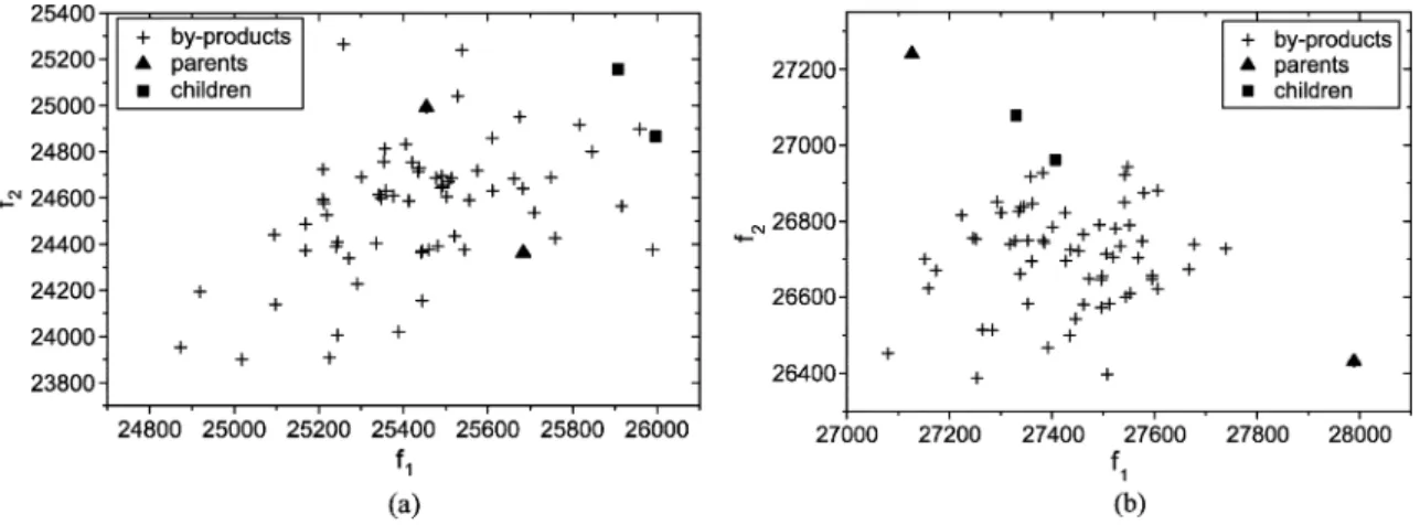
Fig. 2. Examples of an IGC operation in solving a bi-objective maximization problem. (a) Good children can be efficiently generated by the multiobjective IGC. (b) IGC can obtain a well-distributed Pareto front by generating nondominated individuals in the gap between two parents.
value using GPSIFF for a bi-objective minimization problem. For example, three individuals are dominated by and two individuals dominate . Therefore, the fitness value of is . It can be found that one individual has a larger fitness value if it dominates more individuals. On the contrary, one individual has a smaller fitness value if more individuals dominate it.
C. IEA
IEA with IGC is designed toward being an efficient general-purpose optimization algorithm for solving LPOPs. Of course, domain knowledge, heuristics, and auxiliary genetic operations, which can enhance the conventional EAs can also improve the performance of IEA. The simple IEA can be written as follows. Step 1) Initialization: Randomly generate an initial
popula-tion of individuals.
Step 2) Evaluation: Compute fitness values of all individuals.
Step 3) Selection: Perform a conventional selection opera-tion. For example, truncation selection is used: the best individuals are selected to form a new population, where is a selection probability. Let be the best individual in the population. Step 4) Recombination: Randomly select parents
including for IGC, where is a recombina-tion probability. Perform the IGC operarecombina-tions for all selected pairs of parents.
Step 5) Mutation: Apply a conventional mutation operation (e.g., bit-inverse mutation) with a mutation proba-bility to the population. To prevent the best fit-ness value from deteriorating, mutation is not ap-plied to the best individual.
Step 6) Termination test: If a stopping condition is satisfied, stop the algorithm. Otherwise, go to Step 2).
D. IMOEA
Since it has been recognized that the incorporation of elitism may be useful in maintaining diversity and improving the per-formance of multiobjective EAs [26]–[29], IMOEA uses an elite set with capacity to maintain the best nondominated
individuals generated so far. The simple IMOEA can be written as follows.
Step 1) Initialization: Randomly generate an initial popula-tion of individuals and create an empty elite set and an empty temporary elite set . Step 2) Evaluation: Compute all objective function values
of each individual in the population. Assign each individual a fitness value by using GPSIFF. Step 3) Update elite sets: Add the nondominated
individ-uals in both the population and to , and empty . Considering all individuals in , remove the dominated ones. If the number of nondomi-nated individuals in is larger than , ran-domly discard excess individuals.
Step 4) Selection: Select individuals from the population using binary tournament selection and randomly select individuals from to form a
new population, where . If
, let .
Step 5) Recombination: Perform the IGC operations for selected parents. For each IGC opera-tion, add nondominated individuals derived from by-products OA combinations (by-products) and two children to .
Step 6) Mutation: Apply a conventional mutation operation with to the population.
Step 7) Termination test: If a stopping condition is satisfied, stop the algorithm. Otherwise, go to Step 2). If many nondominated solutions are needed, especially in solving large MOOPs with many objectives, one may use an additional external set to store all the nondominated individuals found so far.
Fig. 2 illustrates two typical examples gleaned from the IGC operation using an with in solving a bi-ob-jective 0/1 knapsack problem, described in Section VI. Fig. 2 reveals the following.
1) For one IGC operation, the two children are more promising to be new nondominated individuals, as shown in Fig. 2(a). The individuals corresponding to OA combinations are called by-products of IGC. Because the by-products are well planned and systematically
TABLE III
PERFORMANCE OFVARIOUSEAS FORSOLVING ANLPOP WITH AGLOBALOPTIMUM121.598
TABLE IV BENCHMARKFUNCTIONS
sampled within the hypercube formed by parents, some of them are promising to be nondominated individ-uals. For example, there are three and four by-products being nondominated individuals in Fig. 2(a) and (b), respectively.
2) If the final Pareto front obtained has a gap without sufficient solutions, two nondominated individuals com-prising the gap can be chosen as parents of IGC to fill the gap, as shown in Fig. 2(b). For one IGC operation, the number of nondominated individuals is increased
from two to eight, including two parents, two children, and four by-products.
V. PERFORMANCECOMPARISONS OFIEA
We use three experiments to evaluate the performance of IEA by comparing with some existing EAs without heuristics using benchmark functions consisting of various numbers of
TABLE V
MEANFITNESSVALUES ANDRANKS FORFUNCTIONSWITHD = 10. THEMINIMAL ANDMAXIMALFITNESS
VALUES OFSOLUTIONS IN30 RUNSARESHOWN INBRACKETS
and . Let be the number of parameters
partici-pated in the division phase and . How
to effectively formulate and solve real-world applications of LPOP using IEA with various variants of IGC can be referred in [18]–[20], and[25].
A. Performance Comparisons on LPOPs
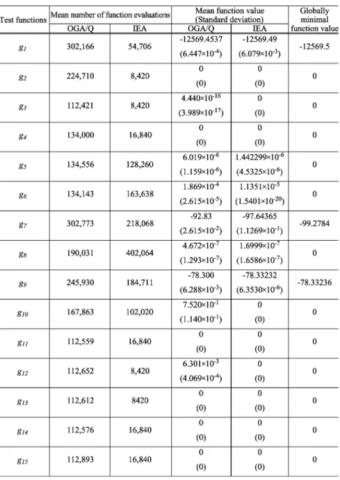
KrishnaKumar et al. [2] proposed three approaches, sto-chastic GA, sensitivity GA, and GA-local search, and provided reasonable success on LPOPs using a multimodal function with no interaction among parameters
(5)
where parameters [3, 13]. The performances of the above-mentioned three methods and a simple genetic algorithm (SGA) are obtained from [2], as shown in Table III. IEA addition-ally compares with the following EAs: BOA [24], a simple GA with elitist strategy using one-point crossover (OEGA), simu-lated annealing GA (SAGA) [30], GA with adaptive probabil-ities of crossover and mutation (AGA) [31], and OGA/Q [8]. Let be the number of fitness evaluations. To directly com-pare with the best one of the three proposed GAs in [2], i.e., the stochastic GA, we specify , chromosome length 500, and the stopping condition using for the compared EAs, except BOA and OGA/Q. For obtaining high performance by using the suggested moderate population size,
BOA uses [24] and OGA/Q uses [8].
The average performances of all compared EAs using ten inde-pendent runs are shown in Table III.
TABLE VI
MEANFITNESSVALUES ANDRANKS FORFUNCTIONSWITHD = 100. THEMINIMAL ANDMAXIMALFITNESS
VALUES OFSOLUTIONS IN30 RUNSARESHOWN INBRACKETS
For BOA, a commonly used constraint restricts the networks to have at most ( in this test) incoming edges into each node. The truncation selection with % is used. The solu-tion of BOA is only superior to those of SGA, OEGA, AGA, and SAGA. BOA averagely takes about 1,115.95 s for a single run, while the other EAs only take less than 1 s using the CPU AMD 800 MHz. It reveals that BOA is hard to solve LPOPs within a limited amount of computation time.
OGA/Q applies the orthogonal design to generate an initial population of points that are scattered uniformly over the fea-sible solution space, so that the algorithm can evenly scan the search space once to locate good points for further exploration in subsequent iterations [8]. OGA/Q divides the feasible solu-tion space along one of all dimensions into subspaces, and
then employs an of Q levels with rows and
columns to generate points in each subspace. In this
test, and . OGA/Q generates
individ-uals and selects combinations having the best fit-ness performance as the initial population. Therefore, OGA/Q
takes to generate an initial
popula-tion. The best solution among the initial population is 110.715. OGA/Q uses an orthogonal crossover with quantization which acts on two parents. The crossover operator quantizes the so-lution space defined by these parents into a finite number of points, and then applies orthogonal design to select a small, but representative sample of points as the potential offspring. For obtaining the optimum 121.598, OGA/Q using 1000 iterations has a mean fitness value 121.594. OGA/Q can obtain an accurate solution but a large number of fitness evaluations are needed.
IEA obtains the best mean solution 120.890, compared with all EAs. For evaluating the ability to obtain an optimal or near-optimal solution, the chromosome length is increased to 1400. Using the stopping condition that the global optimal solution
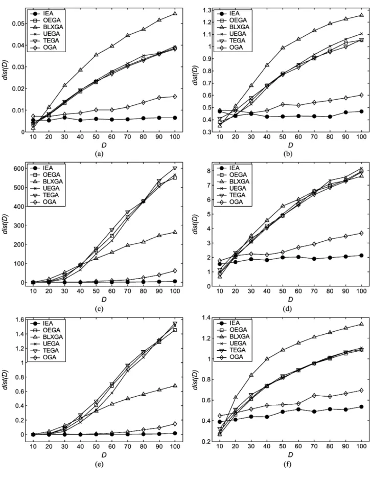
Fig. 3. Comparisons of various GAs usingdist(D) curves for functions f ; f ; . . ., and f in (a), (b), . . ., and (l), respectively.
121.598 is obtained, IEA averagely spends 58 156 fitness eval-uations. The experiment shows that IEA can efficiently search for a very good solution to the LPOP with low epistasis.
B. Test Functions With Various Dimensions
To evaluate the efficiency of IGC for solving optimization problems with various dimensions, 12 benchmark functions
Fig. 3. (Continued.) Comparisons of various GAs usingdist(D) curves for functions f ; f ; . . ., and f in (a), (b), . . ., and (l), respectively.
gleaned from literature, including unimodal, and multimodal functions, as well as continuous and discontinuous functions, are tested in the experimental study. The test function, pa-rameter domain, and global optimum for each function are listed in Table IV. Each parameter is encoded using 10 bits for all test functions except that functions and use
24 bits. The dimensions of the twelve test functions vary on in the experiments. For all compared
EAs, , , , and . The
stopping condition uses .
To compare IGC with commonly used crossover operators without heuristics, one-point, two-point, uniform,
BLX-TABLE VII
PERFORMANCECOMPARISONS OFOGA/QANDIEA
[32], and orthogonal [33] crossover operators are used. Due to the long computation time, BOA is tested on the twelve test functions with only. The compared EAs with elitist strategy and the associated crossover are denoted as (IEA, IGC), (OEGA, one-point), (TEGA, two-point), (UEGA, uniform), (BLXGA, BLX- ), and (OGA, orthogonal).
OGA divides each parent string into parts, sample these parts from parents based on the combinations in an
to produce binary strings, and then select of them to be the offspring. In this experiment, we use the OA and . The comparisons of average performance using 30 indepen-dent runs for and are listed in Tables V and VI, respectively. To illustrate the performance comparisons on var-ious numbers of parameters, we use a distance function
for describing the mean distance between the optimal solution
and the obtained best solution for one param-eter as follows:
(6) The results of average performance for all test functions with
are shown in Fig. 3.
Table V reveals that BOA and OEGA have the best perfor-mances with final ranks 1 and 2, respectively. However, BOA is only slightly superior to OEGA according to the averaged rank, but the computation time of BOA is much longer than that of OEGA. On the other hand, IEA and OGA have the worst perfor-mances with final ranks 6 and 7, respectively. The two OA-based algorithms take more fitness evaluations for one recombination operation than conventional EAs but cannot effectively take ad-vantage of OA experiments in solving the small-scale
optimiza-Fig. 4. Box plots based on the cover metric for multiobjective 0/1 knapsacks problems. The box plot relates to {(2, 250), (3, 250), (4, 250), (2, 500), (3, 500), (4, 500), (2, 750), (3, 750), (4, 750)} (knapsack, item) problems from left to right. Each rectangle refers to algorithmA associated with the corresponding row and algorithmB associated with the corresponding column and gives nine box plots representing the distribution of the cover metric C(A; B). The scale is 0 at the bottom and 1 at the top per rectangle.
tion problems with . Note that IEA is superior to OGA for most test functions. From the simulation results, it can be found that SGA with elitist strategy using one-point crossover (OEGA) performs well in solving small parameter optimization problems.
Table VI reveals that IEA and OGA having the averaged ranks 1.00 and 2.00, respectively, outperform all other EAs. In fact, it can be found from Fig. 3 that IEA and OGA have averaged ranks 1.00 and 2.00 not only for , but also for
. These simulation results reveal the following. 1) The OA-based recombination operations of IEA and
OGA using sampling representative candidate solutions perform well in solving optimization problems with a large number of parameters.
2) IGC performs better than the orthogonal crossover of OGA. It reveals that the reasoned combination using factor analysis is effective in IGC.
3) The mean distance value of IEA slightly in-creases, while increases from 10 to 100, compared with other EAs. IEA can effectively solve LPOPs in a reasonable among of computation time.
4) Fig. 3 reveals that the curves of OEGA, TEGA, and UEGA form a group and the value obviously in-creases, while increases. The performance of BLXGA is similar to those of the three SGAs. It means that the conventional SGA is impractical for solving LPOPs.
Fig. 5. Pareto fronts of the problem with two knapsacks and 750 items.
C. Comparisons With OGA/Q
In Section V-B, it has been shown that IEA is superior to OGA with a randomly generated initial population. In this sec-tion, IEA is compared with OGA/Q by examining the effective-ness of IGC with an OA-based initial population. For compar-ison with OGA/Q, the test functions are the same as those in [8]. The OA-based initial population of IEA is similar to that of OGA/Q, described as follows. After generating points in each subspace like the method of OGA/Q, we further use
factor analysis of OED to estimate main effects of all param-eters with levels and generate an additional point as an in-dividual for each subspace using a reasoned combination of all parameters with the best level. Therefore, IEA use
fitness evaluations in generating an initial population. IEA uses
, where for , , , , , and
for the others according to the domain size as those of OGA/Q. A parameter is encoded using 14 bits. The stopping condition is that when the given optimal value is reached or the best solution cannot be effectively improved in successive 30 iterations. The performance comparisons of IEA and OGA/Q using 50 independent runs are given in Table VII, where the re-ported results of OGA/Q are obtained from [8].
Let and be the initial populations generated using the methods of OGA/Q and IEA, respectively. Let be an individual with an optimal solution. All test functions can be categorized into four classes by carefully examining the simu-lation results as follows:
1) Functions , , , , , : exists in both
and . Therefore, IEA and OGA/Q can ob-tain the optimal solution with a zero standard deviation.
2) Functions , , : exists in but not in
. This means that IGC using factor analysis can efficiently collect optimal values of individual parame-ters, which are distributed in the population, to generate
an .
3) Functions , , : does not exist in either or , and there exists no interaction among parameters. IEA performs better than OGA/Q in terms of both solution quality and computation cost.
4) Functions , , : does not exist in either or , and there exists interactions among parameters. IEA performs better than OGA/Q. For reducing the degree of epistasis of , IEA replaces the square operation with an absolute one using the following fitness function such that IEA can easily obtain the optimal solution to , where ,
, and :
(7)
VI. PERFORMANCECOMPARISONS OFIMOEA The performance of IMOEA is evaluated by the multiob-jective 0/1 knapsack problems and test functions. There are several state-of-the-art methods in the MOEA literature [27], [34]–[45]; we compared against the following subset of these: SPEA [27], SPEA2 [34], NSGA [35], NSGA2 [36], NPGA [37], and VEGA [38]. The cover metric of two nondominated solution sets obtained by two algorithms and is used for performance comparison [27]
the number of individuals in weakly dominated by the number of individuals in (8)
The value means that all individuals in are weakly dominated by . On the contrary, de-notes that none of individuals in is weakly dominated by . Because the cover metric considers weak dominance relation-ship between two sets of algorithms and , is not
necessarily equal to .
A. Multiobjective 0/1 Knapsack Problems
The multiobjective 0/1 knapsack problems have been fully described in [27], and the comparison results demonstrated that SPEA outperforms NSGA, VEGA, NPGA, HLGA [44], and FFGA [45]. Generally, each investigated problem consists of knapsacks, a set of items, weight and profit associated with each item, and an upper bound for the capacity of each knap-sack. The task of the multiobjective 0/1 knapsack problem is to find a subset of items, which can maximize the profits of knapsacks.
The multiobjective 0/1 knapsack problems are formulated as follows. Given a set of knapsacks and a set of items, with the following:
profit of item according to knapsack ; weight of item according to knapsack ; capacity of knapsack ;
find a vector , that
(9)
where and are random integers in the interval [10, 100],
and .
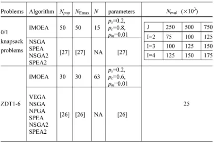
The test data sets are available from the authors [27]. The pa-rameter settings of NSGA2 and SPEA2 are the same as those in [27]. The parameter settings of IMOEA are listed in Table VIII. The chromosomes of IMOEA are encoded uses a binary string of bits, which are divided into gene segments. A greedy repair method adopted in [27] is applied that the re-pair algorithm removes items from the infeasible solutions step by step until all capacity constraints are fulfilled. The order in which the items are deleted is determined by the maximum profit/weight ratio per item. Thirty independent runs of IMOEA are performed per test problem using the same number as that of SPEA. The test problems and reported results of SPEA are directly gleaned from the authors’ website.
The direct comparisons of each independent run between IMOEA and all compared EAs based on the cover metric from 30 runs are depicted using box plots, as shown in Fig. 4. A box plot provides an excellent visual result of a distribution. The box stretches from the lower hinge (defined as the 25th per-centile) to the upper hinge (the 75th perper-centile) and, therefore, contains the middle half of the scores in the distribution. The median is shown as a line across the box. For a typical example, Pareto fronts of the problem with two knapsacks and 750 items merged from 30 runs for IMOEA, SPEA, SPEA2, and NSGA2
TABLE VIII
PARAMETERSETTINGS OFMULTIOBJECTIVEEAS. FOR THEDETAILPARAMETERSETTINGS OF THECOMPAREDEAS, PLEASEREFER TO[26]AND[27]
are shown in Fig. 5. Figs. 4 and 5 reveal the superiority of IMOEA over the compared EAs in terms of robustness and nondominated solution quality. The experimental results reveal that IMOEA outperforms SPEA, SPEA2, and NSGA2, espe-cially for problems with a large number of items (parameters). IMOEA also performs well for various numbers of knapsacks (objectives).
B. Test Functions With Various Problem Features
Deb [46] has identified several problem features that may cause difficulties for multiobjective algorithms in converging to the Pareto-optimal front and maintaining population diversity in the current Pareto front. These features are multimodality, de-ception, isolated optima and collateral noise, which also cause difficulties in single-objective EAs. Following the guidelines, Zitzler et al. [26] constructed six test problems involving these features, and investigated the performance of various popular multiobjective EAs. The empirical results demonstrated that SPEA outperforms NSGA, VEGA, NPGA, HLGA, and FFGA in small-scale problems.
Each of the test problems is structured in the same manner and consists of three functions , , [41]
minimize s.t.
where (10) where is a function consisted of the first decision variable only, is a function of the remaining parameters, and the two parameters of the function are the function values of and . Six test problems can be retrieved from [41].
There are parameters in each test problem. Each parameter in chromosomes is represented by 30 bits, except the parameters
are represented by 5 bits for the deceptive problem .
The experiments in Zitzler’s study indicate that the test problems , , and cause difficulties to evolve a well-distributed Pareto-optimal front. In their experiments, the reports are absent about the test problems with a large number of parameters. As a result, the extended test problems with a large number of parameters are further tested in order to compare the performance of various algorithms in solving large MOOPs. Thirty independent runs were performed using the same stopping criterion as that of SPEA, where . The parameter settings of various algorithms are listed in Table VIII. VEGA, NPGA, NSGA, SPEA, NSGA2, and SPEA2 are the same as those in [26], summarized as
fol-lows: , , , , and
. The population size and the external population size of SPEA are 80 and 20, respectively. For the test problem , the sharing factor of NSGA is 34. The parameter
settings of IMOEA are: , , ,
, , and .
The nondominated solutions merged from 30 runs of VEGA, NPGA, NSGA, NSGA2, SPEA, SPEA2, and IMOEA in the ob-jective space are reported, as shown in Figs. 6–11, and the curve in each figure is the Pareto-optimal front of each test problem ex-cept . The direct comparisons of each independent run be-tween IMOEA and all compared EAs based on the cover metric for 30 runs are depicted in Fig. 12.
For test problems , , and , IMOEA,
SPEA2, and NSGA2 can obtain well-distributed Pareto fronts, and the Pareto fronts of IMOEA for and are very close to the Pareto-optimal fronts. For the multimodal test problem , only IMOEA can obtain a better Pareto front which is much closer to the Pareto-optimal front, compared with the other algorithms. The well-distributed nondominated solutions resulted from that IGC has well-distributed by-prod-ucts which are nondominated solutions at that time. For , IMOEA, SPEA2, and NSGA2 obtained widely distributed
Fig. 6. Convex test problemZDT .
Fig. 7. Nonconvex test problemZDT .
Fig. 8. Discrete test problemZDT .
Pareto fronts, while VEGA failed. The comparisons for indicate that IMOEA is the best algorithm; the next ones are SPEA2, NSGA2, NSGA, and NPGA, while SPEA and VEGA are the worst ones. For , IMOEA also obtained a widely distributed front and IMOEA’s solutions dominate all the solutions obtained by the other algorithms. Finally, it can be observed from [26] and our experiments that when the number of parameters increases, difficulties may arise in evolving a
Fig. 9. Multimodal test problemZDT .
Fig. 10. Deceptive test problemZDT .
Fig. 11. Nonuniform test problemZDT .
well-distributed nondominated front. Moreover, it is observed that VEGA obtained some excel solutions in the objective in some runs of , , and , as shown in Fig. 12. This phenomenon agrees with [8] and [47] that VEGA may converge to individual champion solutions only.
As shown in Figs. 6–12, the quality of nondominated solu-tions obtained by IMOEA is superior to those of all compared
Fig. 12. Box plots based on the cover metric for multiobjective parametric problems. The leftmost box plot relates to ZDT1, the rightmost to ZDT6. Each rectangle refers to algorithmA associated with the corresponding row and algorithm B associated with the corresponding column and gives six box plots representing the distribution of the cover metricC(A; B). The scale is 0 at the bottom and 1 at the top per rectangle.
EAs in terms of the number of nondominated solutions, the distance between the obtained Pareto front and Pareto-optimal front, and the distribution of nondominated solutions. Fig. 12 reveals that the nondominated solutions obtained by IMOEA dominate most of the nondominated solutions obtained by all compared EAs. On the other hand, only few nondominated so-lutions of IMOEA are dominated by the nondominated soso-lutions of all compared EAs.
VII. CONCLUSION
In this paper, we have proposed two intelligent evolutionary algorithms IEA and IMOEA using a novel intelligent gene collector IGC to solve large parameter optimization problems (LPOPs) with single and multiobjective functions, respectively. IGC uses a divide-and-conquer mechanism based on orthog-onal experimental design (OED) to solve LPOPs. Since OED is advantageous for the problems with weak interactions among parameters and IEA/IMOEA works without using linkage identification, it is essential to encode parameters into chro-mosomes such that the degree of epistasis can be minimized. Generally, the problem’s domain knowledge is necessarily incorporated to effectively achieve this goal. Furthermore, maintaining feasibility of all candidate solutions corresponding to the conducted and reasoned combinations of OED can en-hance the accuracy of factor analysis for constrained problems. Modifying genetic operator and repairing strategies can be conveniently used for maintaining feasibility. IMOEA works
well for efficiently finding a set of Pareto-optimal solutions to a generalized multiobjective optimization problem with a large number of parameters. IMOEA is powerful based on the abilities of the proposed GPSIFF and IGC. We believe that the auxiliary techniques, which can improve performance of conventional EAs, can also improve performances of IEA and IMOEA. It is shown empirically that IEA and IMOEA have high performance in solving benchmark functions comprising many parameters, as compared with some existing EAs. Due to its simplicity, theoretical elegance, generality, and superi-ority, IEA and IMOEA can be most widely used for solving real-world applications of LPOPs.
ACKNOWLEDGMENT
The authors would like to thank the editor and the anonymous reviewers for their valuable remarks and comments that helped us to improve the contents of this paper.
REFERENCES
[1] T. Bäck, D. B. Fogel, and Z. Michalewicz, Handbook of Evolutionary
Computation. New York: Oxford, 1997.
[2] K. KrishnaKumar, S. Narayanaswamy, and S. Garg, “Solving large pa-rameter optimization problems using a genetic algorithm with stochastic coding,” in Genetic Algorithms in Engineering and Computer Science, G. Winter, J. Périaux, M. Galán, and P. Cuesta, Eds. New York: Wiley, 1995.
[3] D. Thierens, D. E. Goldberg, and Â. G. Pereira, “Domino convergence, drift, and the temporal-salience structure of problems,” in Proc. 1998
[4] S. H. Park, Robust Design and Analysis for Quality
Engi-neering. London, U.K.: Chapman & Hall, 1996.
[5] T. P. Bagchi, Taguchi Methods Explained: Practical Steps to Robust
De-sign. Englewood Cliffs, NJ: Prentice-Hall, 1993.
[6] A. S. Hedayat, N. J. A. Sloane, and J. Stufken, Orthogonal Arrays:
Theory and Applications. New York: Springer-Verlag, 1999. [7] A. Dey, Orthogonal Fractional Factorial Designs. New York: Wiley,
1985.
[8] Y. W. Leung and Y. P. Wang, “An orthogonal genetic algorithm with quantization for global numerical optimization,” IEEE Trans. Evol.
Comput., vol. 5, pp. 41–53, Feb. 2001.
[9] G. Taguchi, Introduction to Quality Engineering: Designing Quality Into
Products and Processes. Tokyo, Japan: Asian Productivity Organiza-tion, 1986.
[10] M. S. Phadke, Quality Engineering Using Robust Design. Englewood Cliffs, NJ: Prentice-Hall, 1989.
[11] A. Kunjur and S. Krishnamurty, “A robust multicriteria optimization ap-proach,” Mech. Mach. Theory, vol. 32, no. 7, pp. 797–810, 1997. [12] D. M. Osborne and R. L. Armacost, “Review of techniques for
op-timizing multiple quality characteristics in product development,”
Comput. Ind. Eng., vol. 31, no. 1–2, pp. 107–110, 1996.
[13] J. Antony, “Multiresponse optimization in industrial experiments using Taguchi’s quality loss function and principal component analysis,” Int.
J. Qual. Reliab. Eng., vol. 16, no. 1, pp. 3–8, 2000.
[14] E. A. Elsayed and A. Chen, “Optimal levels of process parameters for products with multiple characteristics,” Int. J. Prod. Res., vol. 31, no. 5, pp. 1117–1132, 1993.
[15] A. A. Song, A. Mathur, and K. R. Pattipati, “Design of process parame-ters using robust design techniques and multiple criteria optimization,”
IEEE Trans. Syst., Man, Cybern., vol. 25, pp. 1437–1446, Dec. 1995.
[16] A. P. Wierzbicki, “The use of reference objectives in multiobjective op-timization,” in Multiple Criteria Decision Making, Theory and
Appli-cations, A. P. Fandel and A. P. Gal, Eds. New York: Springer-Verlag, 1980.
[17] S. Rochet, “Epistasis in genetic algorithms revisited,” Inform. Sci., vol. 102, pp. 133–155, 1997.
[18] S.-Y. Ho and Y.-C. Chen, “An efficient evolutionary algorithm for ac-curate polygonal approximation,” Pattern Recognit., vol. 34, no. 12, pp. 2305–2317, 2001.
[19] H.-L. Huang and S.-Y. Ho, “Mesh optimization for surface approxima-tion using an efficient coarse-to-fine evoluapproxima-tionary algorithm,” Pattern
Recognit., vol. 36, no. 5, pp. 1065–1081, 2003.
[20] S.-Y. Ho, C.-C. Liu, and S. Liu, “Design of an optimal nearest neighbor classifier using an intelligent genetic algorithm,” Pattern Recognit. Lett., vol. 23, no. 13, pp. 1495–1503, Nov. 2002.
[21] Q. Wu, “On the optimality of orthogonal experimental design,” Acta
Math. Appl. Sinica, vol. 1, no. 4, pp. 283–299, 1978.
[22] Z. Michalewicz, D. Dasgupta, R. G. Le Riche, and M. Schoenauer, “Evo-lutionary algorithms for constrained engineering problems,” Comput.
Ind. Eng., vol. 30, no. 4, pp. 851–870, Sept. 1996.
[23] D. E. Goldberg, Genetic Algorithms in Search, Optimization and
Ma-chine Learning. Reading, MA: Addison-Wesley, 1989.
[24] M. Pelikan, D. E. Goldberg, and E. Cantu-Paz, “BOA: The Bayesian optimization algorithm,” in Proc. 1st Conf. GECCO-99, 1999, pp. 525–532.
[25] S.-Y. Ho, H.-M. Chen, S.-J. Ho, and T.-K. Chen, “Design of accurate classifiers with a compact fuzzy-rule base using an evolutionary scatter partition of feature space,” IEEE Trans. Systems, Man, Cybern. B, vol. 34, pp. 1031–1044, Apr. 2004.
[26] E. Zitzler, K. Deb, and L. Thiele, “Comparison of multiobjecctive evolu-tionary algorithms: Empirical results,” Evol. Comput., vol. 8, no. 2, pp. 173–195, 2000.
[27] E. Zitzler and L. Thiele, “Multiobjective evolutionary algorithms: A comparative case study and the strengthen Pareto approach,” IEEE
Trans. Evol. Comput., vol. 3, pp. 257–271, Nov. 1999.
[28] K. Deb, Multiobjective Optimization Using Evolutionary
Algo-rithms. New York: Wiley, 2001.
[29] D. A. Van Veldhuizen and G. B. Lamont, “Multiobjective evolutionary algorithms: Analyzing the state-of-the-art,” Evolut. Comput., vol. 8, no. 2, pp. 125–147, 2000.
[30] H. Esbensen and P. Mazumder, “SAGA: A unification of the genetic algorithm with simulated annealing and its application to macro-cell placement,” in Proc. IEEE Int. Conf. VLSI Design, 1994, pp. 211–214.
[31] M. Srinivas and L. M. Patnaik, “Adaptive probabilities of crossover and mutation in genetic algorithms,” IEEE Trans. Systems, Man, Cybern., vol. 24, pp. 656–667, Apr. 1994.
[32] L. J. Eshelman and J. D. Schaffer, Real-Coded Genetic Algorithms and
Interval Schemata. Foundation of Genetic Algorithm-2, L. D. Whitley,
Ed. San Mateo, CA: Morgan Kaufmann, 1993.
[33] Q. Zhang and Y. W. Leung, “An orthogonal genetic algorithm for multi-media multicast routine,” IEEE Trans. Evol. Comput., vol. 3, pp. 53–62, Apr. 1999.
[34] E. Zitzler, M. Laumanns, and L. Thiele et al., “SPEA2: Improving the strength Pareto evolutionary algorithm,” in Proc. EUROGEN
2001—Evolutionary Methods for Design, Optimization and Control With Applications to Industrial Problems, K. C. Giannakoglou et al.,
Eds., 2001, pp. 95–100.
[35] N. Srinivas and K. Deb, “Multiobjective optimization using nondomi-nated sorting in genetic algorithms,” Evol. Comput., vol. 2, no. 3, pp. 221–248, 1994.
[36] K. Deb, A. Pratap, S. Agarwal, and T. Meyarivan, “A fast and elitist mul-tiobjective genetic algorithm: NSGA-II,” IEEE Trans. Evol. Comput., vol. 6, pp. 182–197, Apr. 2002.
[37] J. Horn, N. Nafplotis, and D. E. Goldberg, “A niched Pareto genetic al-gorithm for multiobjective optimization,” in Proc. IEEE Int. Conf.
Evo-lutionary Computation, 1994, pp. 82–87.
[38] J. D. Schaffer, “Multiobjective optimization with vector evaluated genetic algorithms,” in Proc. 1st Int. Conf. Genetic Algorithms, J. J. Grefenstette, Ed., Hillsdale, NJ, 1985, pp. 93–100.
[39] H. Ishibuchi and T. Murata, “A multiobjective genetic local search algo-rithm and its application to flowshop scheduling,” IEEE Trans. Systems,
Man, and Cybern. C: Applications Reviews, vol. 28, pp. 392–403, Aug.
1998.
[40] A. Jaszkiewicz, “Genetic local search for multiple objective combinato-rial optimization,” Inst. Comput. Sci., Poznan Univ. Technol., Poznan, Poland, Res. Rep., RA-014/98, Dec. 1998.
[41] D. W. Corne, J. D. Knowles, and M. J. Oates, “The Pareto-envelope based selection algorithm for multiobjective optimization,” in Proc. 6th
Int. Conf. Parallel Problem Solving From Nature (PPSN VI), 1998, pp.
839–848.
[42] J. D. Knowles and D. W. Corne, “Approximating the nondominated front using Pareto archived evolution strategy,” Evol. Comput., vol. 8, no. 2, pp. 149–172, 2000.
[43] , “M-PAES: A memetic algorithm for multiobjective optimization,” in Proc. Congr. Evolutionary Computation, San Diego, CA, July 16–19, 2000, pp. 325–332.
[44] P. Hajela and C.-Y. Lin, “Genetic search strategies in multicriterion op-timal design,” Struct. Opt., no. 4, pp. 99–107, 1992.
[45] C. M. Fonseca and P. J. Fleming, “Genetic algorithms for multiobjective optimization: Formulation, discussion and generalization,” in Proc. 5th
Int. Conf. Genetic Algorithms, S. Forrest, Ed., San Mateo, CA, 1993, pp.
416–423.
[46] K. Deb, “Multiobjective genetic algorithms: Problem difficulties and construction of test problems,” Evol. Comput., vol. 7, no. 3, pp. 205–230, 1999.
[47] C. A. C. Coello, “A comprehensive survey of evolutionary-based mul-tiobjective optimization techniques,” Int. J. Knowl. Inform. Syst., vol. 1, no. 3, pp. 269–308, 1999.
Shinn-Ying Ho (M’00) was born in Taiwan,
R.O.C., in 1962. He received the B.S., M.S., and Ph.D. degrees in computer science and information engineering from the National Chiao Tung Univer-sity, Hsinchu, Taiwan, in 1984, 1986, and 1992, respectively.
From 1992 to 2004, he was a Professor in the De-partment of Information Engineering and Computer Science, Feng Chia University, Taichung, Taiwan, R.O.C. He is currently a Professor in the Department of Biological Science and Technology, Institute of Bioinformatics, National Chiao Tung University, Hsinchu, Taiwan, R.O.C. His research interests include evolutionary algorithms, image processing, pattern recognition, bioinformatics, data mining, virtual reality applications of computer vision, fuzzy classifier, large parameter optimization problems, and system optimization.
Li-Sun Shu (S’04) was born in Taiwan, R.O.C., in
1972. He received the B.A. degree in mathematics from Chung Yuan University, Taoyuan, Taiwan, in 1995 and the M.S. and Ph.D. degrees in information engineering and computer science from Feng Chia University, Taichung, Taiwan, R.O.C., in 1997 and 2004, respectively.
He is a Lecturer at the Overseas Chinese Institute of Technology, Taichung, Taiwan, R.O.C. His re-search interests include evolutionary computation, large parameter optimization problems, fuzzy sys-tems, and system optimization.
Jian-Hung Chen (S’00) was born in Chai-Yi,
Taiwan, R.O.C., in 1974. He received the B.A. degree in surveying engineering from National Cheng Kung University, Tainan, Taiwan, in 1997 and the Ph.D. degree in information engineering and computer science from Feng Chia University, Taichung, Taiwan, R.O.C., in 2004.
From 2001 to 2002, he was with the Illinois Genetic Algorithms Laboratory, University of Illi-nois, Urbana–Champaign. His research interests include evolutionary computation, multiobjective optimization, pattern recognition, data mining, flexible manufacturing systems, resources planning, experimental design, and system optimization.
Dr. Chen was the recipient of the Taiwan Government Visiting Scholar Fel-lowship in 2000. He was the recipient of the IEEE Neural Networks Society Walter Karplus Research Grant (2003).