EXPLOITATIVE COMPETITION OF MICROORGANISMS FOR 2 COMPLEMENTARY NUTRIENTS IN CONTINUOUS CULTURES

EXPLOITATIVE COMPETITION OF

MICROORGANISMS

FOR TWO

COMPLEMENTARY NUTRIENTS IN

CONTINUOUS

CULTURES*

SZE-BI HSUt, KUO-SHUNG CHENG AND S. P. HUBBELL:I:

Abstract. Thispaper concernstheexploitative competition oftwomicroorganisms for two

complemen-tarynutrients inthecontinuous culture.Consumptionofthe limiting resourcesfollows theHollingType II

functionalresponse or, equivalently,Michaelis-Menten kinetics, generalized to the two-resource situation.

The predicted biologicalconditions whichshould giverise toeachof the possible competitive outcomes are

presentedin detailand analyzedglobally.Amajor conclusion is thateachof thefouroutcomes of classical

Lotka-Volterratwo-species competition theory hasmultiple mechanisticorigins in terms of

consumer-resourceinteractions.Itisalsoshownthat allfourclassical outcomes, including thecasein whichwinning

dependsonthe initialabundancesof thecompetitors, can arise for thispurelyexploitativecompetition.

Moreover,the outcomes of thisexploitativecompetition can bepredicted,inadvanceof actualcompetition, frommeasurementsmadeoneachspeciesgrownbyitselfonthe resources.

1. Introduction. The classical theory of ecological competition between twoor more species, attributed to Lotka

[18]

and Volterra

[36],

is an extension of the basic

logistic model of single-species growththatdatesfrom Verhulst

[35].

The dynamical equationsfor thistheoryfor twocompetitors, 1 and 2, areoften written as

dN

{1-(N+aN2)}

dN2

(1.1)

d---

rlN1

KI

dt 1

(/3N,

+

N)

}

r2N2

K2

where

Ni

isthe numberofthe ithcompeting species,ri and

K

aretheintrinsicrate of increase andthe carrying capacityoftheithcompetitor, respectively, anda

and/3

are

the interaction of "competition" coefficients, expressing the per capita competitive

effect of species 2 on 1, and 1 on 2, respectively. In the absence of competition

(c =/ 0),each populationgrowstoitsrespectivecarrying capacity. Inthe presence

ofcompetition,one orthe otherrivalmaysurvive while itscompetitordiesout,orelse therivalsmaycoexist.These three biologicaloutcomes result from thefour mathemati-cal casesthatcan occurprovided that populations of both speciesarepresentinitially. Competitive stability (coexistence) occurs when a

< K/K2 and/3 <

KE/K1;

competi-tive instability (initial numbers of the competitors determine the eventual winner)

occurswhentheseinequalitiesarebothreversed; and competitivedominance

(one

or

the other specieswinsregardless of initialnumbers) occurswhenone but not both of

these inequalities arereversed.

Theclassical theorycanperhaps be called a"phenomenological" theory insofar

asitseeksto describehow the numbers of competing species change, and topredict the eventual outcome of such competition, without ever being specific about which

limiting resources are the focus of competition, nor about how effectively the rival

species forage for, and exploit, these resources. This classical theory has had an immenseand lastingappeal because ofitsgenerality andsimplicity, andithas been the

subject ofaverylarge numberof theoretical studies(cf.Wangersky’sreview

[38]).

By

thesametoken, however,thisgenerality has also madeit difficultforexperimentalists

to interpret and measure the theory’s critical parameters. It has proven especially *Received bythe editorsMarch 31, 1980, and in revised form December 1, 1980.Thiswork was partiallysupported by theNational Science Council of theRepublicof China.

tDepartment of Applied Mathematics, National Chiao-Tung University, Hsin-Chu, Taiwan 300,

Republicof China.

$DepartmentofZoology, University ofIowa, IowaCity,Iowa52240. 422

difficulttoestimatethe competitioncoefficientsindependently of actually growing the potential competitors together, and to determine theirvalues under fieldconditions, althoughconsiderable attentionhas beendevotedtotheseproblems.Usually,

competi-tion coefficients have.been estimated in laboratory competition studies by fitting the dynamical equations

(1.1)

to the growth curves of the species in competition (e.g.,

Vandermeer

[34]).

The attempts to estimate competition coefficients have usually focused on various measures of overlap in resource utilization (Schoener

[28]),

although information about whether the resources are limiting is usually lacking. Unfortunately, whenever these coefficients canonlybe estimatedfromthe dynamics of populations alreadyincompetition, thevalue ofthe theoryforpredictionisthereby diminished. Thus, the classical theory has been attackedas atautological exercise in

curvefittingatbest

(Peters

[23]).

Atworstthefitof

(1.1)

todataispoor (Wilbur

[39],

Neill

[22],

Richmond et al.

[26])

because of avariety of nonlinearities inper capita

ratesofgrowthas afunctionof competitordensities.

Overthe past 25 years the elementsof a moremechanistic, resource-based theory of ecological competition have been under experimental andtheoreticaldevelopment byadiverse field

ot

workers.

A

list

ot

all significant contributionsto thiseffortwould

bequite long, butsome

ot

themilestoneshave been papers by Herbertetal.

[6],

Powell

[24],

Holling

[7], [8],

[9],

Miller

[21],

Dugdale

[2],

Eppley and Coatsworth

[3],

Epply and Thomas

[4],

Kilham

[14],

MacArthur

[19],

Stewart and Levin

[30], Droop [1],

Koch

[15],

Leonand

Tumpson [17],

Smithetal.

[29],

Taylorand Williams

[31],

Tilman

andKilham

[32],

Tilman

[33],

Real

[25],

andHsuetal.

[10l,

[12].

Thistheoryconsiders

the dynamics of theresourcesexplicitlyin addition tothe population dynamicsofthe competing species.

Moreover,

itpaysparticular attention to thefunctionalresponses

ofthe competitors tochanges inresourcedensity.

Incomparisonwiththeclassicalapproachto competition, some thingsaregained andsome arelostby adoptingthisapproach.The disadvantages are that resource-based competitiontheoryisusuallylessgeneral,butalsomoredifficulttoanalyze

mathemati-cally, thanclassicaltheory.

However,

the advantagesarethatthe experimentalist hasa

specificset ofsomewhat more mechanistic questions toask about limiting resources and themannerin whichthe consumersrespond functionally and numericallytothese

resources.Thus,resource-basedtheory directsmoreexplicitattention toresourcesand consumer-resource interactions thanLotka-Volterra theory which, classicallyatleast, focused primarily if notexclusively onthe phenomenological changes in competitor numbers.

We

believe that this approach will spur renewed interest in experimental

studies of competition, and we also hope that it hastens the development of more predictivetheory.

In

thispaperwepresentaresource-based competition modelwhichdescribes how

twomicroorganisms compete exploitatively for two complementary resources in the chemostat.

A

chemostat isalaboratoryapparatus used for production and physiological studyofmicroorganisms.

In

the chemostat model, the limitingnutrient issuppliedat aconstant rate.The inputflowotmedium containsall other factorsforgrowthin excess.

The output flow equals the input flow, and carries with it cells, waste product and unusednutrient.Themodelalsoapproximatesconditions forplankton growthinlakes,

with the input of complementary limiting nutrients such assilicaand phosphate from

streamsdraining the surrounding watershed.

2. Competitionforone resource. Before consideringtworesources,itisusefulto reviewbriefly whathappensinthe one-resourcecase.

We

assume that the consumption of a single limiting resource follows the Holling

Type II

functional response or,

equivalently, Michaelis-Menten kinetics, which describes the chemical interaction

between enzyme and substrate. When aspecies grows on a single limitingresource, there is some "break-even" concentration of that resource at which birth rate just balances death rate,which we willcall the subsistenceconcentration.Nowsuppose that

this limiting resource is supplied at a constant rate, corresponding to the constant

carrying capacityenvironmentof classicalcompetitiontheory, and thattwospecies

(or

more)

arecompeting exploitatively forthisresource.Then,provided that theresource is not being suppliedata ratebelow the subsistenceconcentrationof all species, only

asingle speciesispredictedtosurvive" that specieswhichhasthe smallestsubsistence concentrationof the resource

(Stewart

andLevin

[30],

Taylor and Williams

[31],

Hsu

et al.

[10]).

Recently Hansen and Hubbell

[5]

conducted a rigorous test of this

prediction. Thisnicelyintuitiveresultturnsout,however, tobedependentonhaving

a constantresource input. If theresourcehasaperiodic input, for example,seasonally

(Stewart

and Levin

[30], Hsu [13]),

or if the resource is a prey species capable of self-reproduction (Koch

[15],

Hsu et al.

[12]),

then there are conditions when the species

can

coexistinadynamic, periodicfashion on asingle resource

(McGehee

and

Armstrong [20]).

Fortheremainder of thispaper,we willbeconcernedwiththe case

ofaconstantcarrying capacity environment, correspondingtoLotka-Volterratheory,

butin resource terms.

Thesubsistenceresourceconcentrationis animportant competition criterion,not

onlyinone-resource situations, butinthetwo-resourcetheorydiscussed in thispaper

aswell.Foreach species and limiting resource, thereissuchaconcentration, potentially

different in each case.Itwillbe symbolized by

J,

following Rosenzweig

[27].

In

ourprevious workon thissubject

10],

11

],

wehave usedA for this parameter, but henceforth wewill use J to avoid confusion withthe finite rateof increase.The

subsistence concentrationcan be calculated from three parameters that are measured

oneach species grown by itself onthe particular resource. Thus, forresources Sand speciesi,

Jsi

canbe found from"

(a)

thehalf-saturation constant forresource uptake, Ksi;

(b)

theintrinsic rateof increase,ri; and

(c)

thedeath rate,

Di.

Thehalf-saturation

constant

Ki

corresponds to K, in Michaelis-Menten theory, and represents that

concentration of resourceat whichconsumption occursathalfthemaximalrate. The

subsistence concentration forspecies growth-limitedby resource Sistheproductof the half-saturation constant and the ratio of the death rate to the intrinsic rate of

increase"

\_rsi/

The units of

Ji

arein resource concentration, since theunitsof

_Di

and rsicancel. The parameter ri isequivalentto

rmax

for theithspecies, rsi (msi-Di), wheremsi isthe

maximalper capitabirthrate onresource S.

For

the detailed biological meaning ofJsi

wereferto

[10].

The equations for single-resource competitionamongn species for resourceSare

d__S (sO)_

S)D

Y. ms--2

S N, dt i= yi

Ksi

+

S

(2.2)

dNi

m,i$"

Ni

DIN/, i=l,2,...,n. dt

Ksi

-t-S

Sisthe concentration ofresource, S)istheconstantinput concentration ofresource,

D

isthe constant rate atwhichnew nutrient is imported, as well as therate at which

nutrientat currentconcentrationisexported.

For

theithorganism,

Ni

isthe population density,

Ysi

isthe yield of the ith organism produced perunitofresourceS consumed,

and

Ks,

m, and

D

areasdefinedabove.Itwillbe recognized that

(2.2)

isthe system of equations for any continuous culture ofseveral species, growth-limited byasingle nutrientbut supplied with all otherrequirednutrients innonlimitingamounts(Taylor

andWilliams

[31], Hsu

et al.

[10],

Hsu

[11]).

This is tobeexpected,sincecontinuous cultures were specifically developed as idealized environments having a constant

carryingcapacity. Thus,itshould be noted that a constantcarrying capacity doesnot

result from a fixed quantity of limiting resource, as in batch culture, but from a

steady-stateresourceinput-outputsituation.

In

(2.2),ifnoorganismsarepresent, then the resource equilibratesat

S

()atthe point when resource input and outputrates are

balanced.

The one-resource situation can be summed up as follows. With no loss of generality, number the competing

species

such thattheir

J’s

areordered, with

_{Js1 <}

Js2

<’

<

_Jsn.

All species dieoutif theinputconcentrationislessthan thesubsistence concentration for every species, i.e., if

S()<Jsl.

In

this case, limt_ooS(t)= S() and

limt_,oo

N(t)-

O,i-1,...,n.

On

the otherhand, if

S()>

Ji for any i,then species 1

survivesand outcompetes all rival species.

In

thiscase,limt_,oo

S(t)

J,

limt_,o

N(t)

y,x(S()-Js)

andlimt_,oo

N(t)=

O, 2,...,n.

3. Competition[or_{two resources.}

In

situationsinvolvingtwo or moreresources,

itbecomes necessary for the firsttime to considerhow the resources,onceconsumed,

interact topromotegrowth.

Leon

and

Tumpson [17]

have distinguishedtwoimportant classes ofresources: complementary andsubstitutable. Complementary resources are

sources of differentessentialsubstanceswhich aremetabolically independent

require-mentsfor growth, suchas a carbon source andanitrogen sourcefor a bacterium,or

silica and phosphorus for a diatom. On the other hand, substitutable resources represent alternate sources of the same essential substance, and are metabolically interdependent requirements for growth, such as two carbon sources or two sources forphosphorous.

In

thispaperwe considerjust thecase ofcomplementaryresources.

Nowconsider twocomplementary resources,

R

andS.

For

eachconsumerspecies thereare twoJ’s,onefor eachresource.TheseJ’sarethesubsistence concentration of

each resource when the species is growth-limited by that one resource alone. For

species i, call theseconcentrations

_Jr

and

J

of resourcesR and

S,

respectively. These

J

valuesdetermine the position of the zero-growthisocline for species on the S-R

resource plane.

Thezero isoclinefor complementaryresources is a pairof half-lines meeting at

rightanglesatthe point

(J,

.]rri)in the

S-R

plane (Fig.

1).

Thelines areperpendicular because ofthe independence of the requirements for

R

and$.

In

thiscase, growthis

limitedatany giventimeeitherby

R

orby

S,

butnotby both

R

andSsimultaneously exceptatthe

corner).

The curving dashedlinepassingthroughthe cornerintheisocline

represents the equation, miS/(Ki

+

.9)

mrR/(K,.

+

R),

where the parametersareas

previouslydefinedbut subscripted for the appropriate resource. Above the dashedline inthetheS-R plane, species isS-limited, whereas below the dashed line, species is R-limited (Fig.

1).

Thus, for example, when species is S-limited, no increase in

resource

R

inthe region above the dashedcurve willhave any effectonincreasing the growth rate of species i; only an increase in resource $ will have this effect. The converse istrue inthe region below the dashedcurve.

Before presenting the competition modelsfor twospecieson twocomplementary resources, we should discuss how the functional responses of the consumer species

Jri

/

i-th predoor isocline

=0

/ msiS mriR

/

/ _{Ks +S Kri+R}

FIG.

have been generalized from one to two resources. In the one-resourcecase, the per capita consumption rate, according to the

Type II

functional response, is given by

(mri/yri)(R/(Kri+R)) if the resource is

R,

or is given by (rnsi/ys)(S/Ks+S))if the resource is $. Now we generalize the functional response to two complementary

resources.

In

this case, the per capita consumption rate of whichever resource is

currentlylimitinggrowthis identical tothe one-resource per capita consumption rate, as given above for the appropriate resource. The question thenarises. Atwhatrate is

the nonlimitingresourceconsumed?Thisquestioncanbeansweredwhenweconsider the yield ofconsumerproducedperunitof resourceconsumed. When the yieldfactors,

Yri and Ys are constants, then it follows that there must be a fixed ratio of the growth-essential substances provided by resources

R

and S in a unit of consumer.

Moreover,

this also implies that the per capita consumption rate of the nonlimiting resource must be proportional to the per capita consumption rate of the limiting resource. Ifit were not, then theratioofessentialgrowth substancesintheconsumer

would be changing, and the yield factors wouldnolongerbeconstant.The proportion-alityconstant is the ratio ofthe yield constants for the two resources. For example, suppose species is S-limited. Then the per capita consumptionrate of

S,

callit

f(S),

is

msi S

(3.1)

_f

(S)

ys, Ks,

+

S’

whereas the concurrentper capita consumptionrate of the nonlimiting resourceR is

given by

(3.2)

Ys--2/’

_f

l(S)

ms____

S

Y

,.

Yr

Ks

+

S

Note that the expression in

(3.2)

does not contain the concentration of the nonlimitingresource

R.

Thus, itshould be noted that:

For

complementary resources

R

and

S,

whena species isS-limited, itspercapitaconsumptionrate

_of

Risindependent

_of

theconcentration

_of

R,

whereas, when thespecies isR-limited,itspercapita consumption rate

_of

S isindependent

_of

theconcentration

_of

$. The keyto this statementis: "When

is aspeciesS-limited?".The speciesisonlyS-limitedabove a certain concentration of

resource

R (above

the dashedline inFig.

1).

Belowthis concentration of

R,

the per capita consumption rate of

R

does depend on the concentration of

R;

but this

dependence is because the species is now R-limited and no longer S-limited. The

converseargumentapplies when the speciesisR-limited.

4.

Statement

of the model. Given the precedingdevelopment of the biological

basisforthe functional response of species exploiting pairsofcomplementary

resour-ces, it is astraightforward matter tostate the two-resource, two-species competition model in the continuous culture.

Forcomplementary resources,

R

and

S,

and species 1 and 2 competing exploita-tively forthem,the system of equationsis

dS 1 1 .-7

S

S)D

g(S, R

)N

g2(S,

R

[a _{Ysl Ys2}

(4.1)

dR 1 1

d---

(R

0

R )D

gl

(S,

R

)NI

g2(S,

R

)N2,

Yrl Yr2

dNa

dNz

=[g(S,R)-D]N, =[g2(S,R)-D]N, dt dt

S(O) >

O,

R (0) >

O,

N(O) >

O,

N2(O) >

O,

where

rnsiS

mrtR

)

g

S, R

min

K-

-

-S

Kr

+

R

(

ms S

mr _R_

g2(S, R

min

I-2--S

Kn

+

R

I"

As

noted previously,this model assumes constantcarrying capacities (fixedrate

of nutrient input), constant yield factors (unit of consumer produced per unit of resourceconsumed),and

Type II

functionalresponses, generalizedto two complemen-tary resources.

In

addition,wehaveassumed

Type II

numericalresponsesinpercapita

birthrates, with a directdependenceonthe external supplyofresources. Finally,we

have assumed the same dilution rate

D

for

S,

R, N, N2.

The parameters in

(4.11)

have all been previously defined atvarious pointsin the text, but itiscon-venient to relist them here in oneplace for ease of reference"

S

,

R

=

input concentrations of resourceS and

R,

respectively.

D

input flow rate of medium containing

S,

R and also the output flow rate mediumcontaining unused

S, R

and cells N1,

N2.

ms, tnr maximalpercapitabirthrateof species onresourceS or

R

alone.

Ysi,Yri yield of species perunitof resourceSorR consumed.

K,

_Kr

half-saturation constantfor species onresource S orR.

We analyze the behavior of solutions of this system of ordinary differential

equations in ordertoanswer the biological question, under whatconditions willneither, one,orboth species surviveordieout?

We

alsoseekto determine thelimiting behavior of the surviving species and the resources.

5.

Statement

ofresults.

In

this section westatethe principal results of thepaper.

The proofs and certain technical lemmas are deferred to 6. The first lemma is a statementthat the system given by

(4.1)

is as "well-behaved" as oneintuits from the

biological problem. Theproof of the lemma is similar tothat in

[10],

and we omitit.

LEMMA5.1. Solutions

o[ (4.1)

are positive and bounded.Furthermore, wehave

(5.1)

S(t)

S() Ng(t)

+o(1)

ast-,

i= _Ysi

(5.2)

R(t)=R(o)_

Ng(t)+o(1)

ast-->eo.

)]ri

The next lemma providesconditions under which the organismscannot survive

given thefixed dilutionrate and thefixedinputrates ofthe nutrients.Beforewestate

the lemma,wenotethe followingtwopairsofequivalentstatements, namely,

msiS

() KsiD

_s(O)

Ksi-Jr-S(0)

<

D ifandonlyif msi<--Dor

msi

D

>

mriR

(o)

KriD

(o)

Kri

-1-

R

(o)

<

D ifand onlyif mri

<=

Dor

mri

D

>

R

LEMMA5.2.

(5.3)

then limt_,oNi(t) O.

msiS

()

mriR

(o)

Ks

q-

s(O)

<

D or

_Kri

-[-R(o)

< D,

Lemma5.2statesthe necessaryconditions forspecies

Ni

tosurvive, i.e.,

KgD

s(O)

K,.D

0<< and

0<<R().

msi D mri D

Since nutrients S and R are complementarily essential to the growth of speciesNi,

there are minimum input concentrations S() and R() both for S and

R

in order to

support the speciesNi.

COROLLARY5.3.

_If

(5.3) holds

_for

1,2, then limt_ooS(t) S

(),

limt_,R (t) R(o)

andlimt_,o_{Ni (t)} O, 1, 2.

We state the principal result in the case of inadequate input concentration of nutrientsin four parts.We areable to determine theglobally asymptoticbehavior of

the solutions in Theorem 5.4. The theorem may be summarized by noting that the unsuccessful competitor doesnot affectthe eventual behaviorof thesurvivor andits

resources.

Beforewestate Theorem 5.4,weintroducethe following important parameters"

Jsi Jri 1,2, msi D mri D

Ci

yi

Ti

R (0) Jri ..,(o) 1 2. Jsi Yri

THEOREM 5.4(i), (ii). Let

(5.3) hold]or

=2 and

O<Jsl

<S

(0),

O<Jrl

<R

().

(i)

_If

T1

<

C1, then the trajectory

of

(4.1)

approaches theequilibrium

(Es

1)

as -->

oe,

where

Nsl*

(Esl)

(JI,

R*

sl,Nsl,*

0),

Nsl

* ysl(S

-Jsl)

R*

R ()

sl (o)

Yrl

(ii)

_If

T1 <

C1, thenthetrajectory

of

(4’1)

approaches theequilibrium(Erl)as

where

(Erl)

(Sr*,

Jrl,

N’r1,

0),

N*

,1

Y,I(R()-

Jl),

THEOREM 5.4(iii), (iv). Let

(5.3)

hold

]’or

i=1 and O(Js2(S

(0),

_O<Jr2<R

().

(iii)

_If

T2

>

C2,thenthe tra]ectory

_of

(4.1)

approaches theequilibrium

(Es2)

as

where

(Es2)

(Js2,

R*

s2,O, N*

s2)

N

*

s2 ys2(S -Js2), R R

(1

,

(o)

Ns2

s2

Yr2

(iv)

_If

T2

< C.,

thenthetrajectory

o

(4.1)

approachesthe equilibrium

(Er2)

as

o,

where

(Er2)

(Sr2,

Jr2,O, N

r*2

N*

r2

Yr2(R

--Jr2),

Sr2

(0)

,

=s(O)Nr*2

Ys2

Theorem 5.4 statesthat whenlimt_,ooNi(t)=0 the equation

(4.1)

isreduced to a

system of three ordinary differential equations.

In

order to present the biological meaningofparameters

T,

Ci, weassume limt_,oo

N2(t)=

0.

We

mayrewrite T1,

C1

as

(R()-Jrl)D

1/yrl

T1

(s(O)_jsl)

D

C1-

1/ysl

When only species 1 is present,

T1

represents the ratio of the steady-state nutrient

regenerationrates atequilibrium under consumption by 1.

Jr1

and

Jsl

arethe

equilib-rium concentrationsofresourcesR and

S,

respectively, understeady-state

consump-tionby species 1. The parameter

C1

represents thefixedyieldratiofor species 1 growing

on resources

R

and S. The units of (1/yrl) are (units

R consumed/unit

species 1

produced); thus

C1

is the ratio, (units R

consumed/units

S

consumed)

per unit of

species 1produced.

By

comparing

T1

with C1, we can determine whether species 1 is S-limited or R-limited. This is because

C1

represents the invariant ratio in which the essential

nutrients

R

andSareconsumed by species1,whereas

T1

represents theratioin which

thesesame resourcesare beingexternallyregeneratedundersteady-stateconsumption

pressurefrom species 1.Therefore,if

T1 >

C1,thegrowthrate ofspecies 1is S-limited

because S is regenerating at a steady-state rate slower than

R

with respect to the required consumptionratiofor species 1. Similarly,if

T1

<

C1,the growthrateof species 1 willbe R-limited. The aboveconsiderationsalsoapplytospecies 2forappropriate values of

_T2

and

C2.

DEFINITION. If

T1

>

C1

(or T1 < C1),

we say that species

N1

is S-limited

(or

R-limited). Similarly, if

T2

>

C2

(or

T2

<

C2), wesay that species

N2

is S-limited

(or

R-limited).

Remark.

We

mayjustify the concept ofR-limited orS-limited.Consider system

(4.1) withN2--0. Suppose N1

isR-limited, thenatequilibrium

(S*rl,

Jr

1,

Nr*l

wehave

D

(mrlJrl)/(Krl

+

Jrl)

<

(mslS*

)/(Ks

+

Srl

*

and henceS

*

>

_Js

Then

mrlJrl

N*rl

yrl(R()-

Jr1

Krl+Jrl

D

YSl(S

(0)

S

_rl

<

Ys

(s(0)

Js

1)

andso

_T1

<

C1.

Similarly, if

N1

is S-limitedthen

C1

<

T.

In order to discuss the interior equilibrium point, we may assume as a basic

hypothesis

(H1)

S() >

Jx,

Js2 >

0,

R()>Jrx,

Jr2>O.

Under the assumption (HI), the equations of

(4.1)

maybe relabeled without loss of

generality,so thatwemay assume either

(H2)

Jl

<Jr2,

Jl

<J2

or

(H3)

J

< Jr,

J2<J.

We

note that most of the conditions on parameters for the various cases in

Theorems,5.5, 5.6canalso beestablishedby thelinearizationmethod.

Beforewestateour mainresults,Theorems5.5and5.6,weintroducethe following parameters"

T*-R()-Jr2

_N*c

ysl(S()-Jsl)(C2-

T*)

Nc

Ys2(S()-JI)(T*-C1)

S(0)

Ys

C1

C1

C2

C1

THEORZM 5.5.

Assume (H1)

and

(H2)

hold

(see

Figs. 2a, 2b). Let

C1

C2.

Then

thestatementsin Theorem 5.4(i) (ii) hold.

R R

Ir2

Jr1

(Esl) GS GS: Globally Stable

.Tr2’

.Trl (Erl) I, =-S I,

JSl

-Ts2

Jsl

Js2

a. N1isS-limited. b. _NisR-limited. FIG.2

Theorem 5.5statesthat,if onespecies has the lowerJ’sfor bothnutrients

S

and

R,

then that specieswill surviveandits rival will not.

Now we consider the situation when each species has the lower subsistence

concentration on one oftheresources, say,

Jr1 <

Jr2,

J2 <

J

1.Then theparameters

T*,

C1

and

C2

become importantinthe competitionoutcomes.

First westate thefollowing results describing howonespeciescanoutcompetethe other.

THEOREM 5.6(i).

Assume (H1)

and

(H3)

hold. Let

C1

C2.

If

T* <

C1, C2, then thestatements in Theorem 5.4(i), (ii) hold

(see

Figs. 3a,

3b).

THEOREM 5.6(ii). Under the assumptions

of

part (i),

if

T*>

C1, C2, then the

statements in Theorem 5.4(iii), (iv) hold

(see

Figs.4a,

4b).

J’r2

Jr1

U: Unstable (Er2) (Es) U

Js2

-Ts

R Jr2 .Trl FIG.3 (Er2)

(E-r1)

Js2 b S GS U

I(Esl)

.Ir2 .Irl GS

(Er2)

Js2

Is1 Is2 a FIG. 4 (Esl)

In

order to explain the biological meaning of Theorem 5.6(i), (ii), we rewrite

T*

(R

(o)

Jra)D/(S

()

Js

1)D,

whichrepresents theratio ofthe steady-state

regener-ationrateof

R

when

N.

isalone and that ofSwhen

Nt

is alone.

We

notethatunder the assumption

(H3)

wehave

T* <

T1

and

T*

>

_Ta.

First weconsider Theorem5.6(i).

The assumption

T* < C,

Ca

implies

Ta

< Ca;

i.e., species

Na

isalwaysR-limited.

But,

since species

N

has the lower subsistenceconcentration for resource

R,

species

Nt

alwayswins.

Note,

however,thatatthe one-species equilibrium, species

N

may again beeither S-limited or R-limited. Similarily,we canexplain Theorem 5.6(ii).Species

N2

outcompetes species

N1

forthereasonthat species

N

is S-limitedand

N2

has the lower subsistence concentration for resourceS.

Secondly,wedescribe howtwospeciescancoexist.

THEOREM 5.6(iii). Under the assumptions

of

part (i).

_ff

C1 < T* <

C2, then the "positive" equilibrium

(E)=

(J,Jr2,

N,

N)

exists and is globally asymptotically stablein the

_first

orthant

(see

Fig.

5).

In

this case, we note that

C

< T,

and

T2

<

C2; i.e.,

N1

is S-limited and

N2

is

R-limited.

But,

species N1,

N2

has lower subsistence concentration for

R

and S

respectively. Coexistence occursbecause eachspecies has the lower subsistence con-centration forthatresourcewhich,atthetwo-speciesequilibriummixtureofresources,

most limitsthegrowthof itsrival.

Jr2

Jr1

U (Es) GS

(E)

Js2 sl (Er2) FIG.5

Finally,westatearesult describing theoutcomeof competition dependsoninitial

populations. Thereare two cases. Thefirstone

((a), (d))

isthecase when both species

are limitedby thesameresource.The secondone((b),

(d))

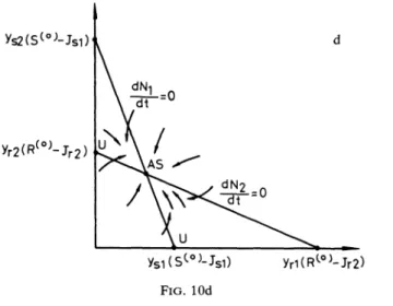
isthecasewhenthe species arelimitedbydifferentresources.

THEOREM 5.6(iv). Under the assumptions

of

part

(i),//C2 < T*<

C1, then

(Ec)

existsandunstable.Furthermore, wehave

_four

possibleoutcomes:

(a)

_If

NI

is S-limitedand

N2

isS-limited, then

(Es)

and

(Es2)

areasymptotically

stable.

(see

Fig.

6a).

]’r2

J’rl

AS (Es2)

U AS

AS: Asymptotically Stable

(Ec) (Esl)

Is2

Isl

Jr2

Jr1 AS, Js2 ,(Es2) (Ec) b (Erl)

;s

.lr2 Jr1 (Er2) (Ec)

u

(Esl) AS

Js2

]sl C FIG. 6 Jr2

Jr1

Er2) (Ec)

A=S U"

/s2

]sl (Erl)

(b)

_If

N1

isR-limitedand

_N2

isS-limited, then

(Erl)

and

(Es2)

are asymptotically stable (see Fig.6b).

(c)

_If

N1

isS-limitedand

N2

isR-limited, then (Esl) and

(Er2)

areasymptotically stable (see Fig.

6c).

(d)

_If

Nx

isR-limitedand

N2

isR-limited, then

(Erx)

and

(Er2)

areasymptotically

stable

(see

Fig.6d).

This case arises because eachspecies has thelower subsistence concentration for

that resource which, atthe two-species equilibrium mixture of resources, leastlimits

the growth ofitsrival.Thismakes the two-species equilibrium unstable. Theoutcomes

dependonwhether species

Nx

and species

N2

areindividually S-limited or R-limited atthe one-species equilibrium.

6. The

Proof of

Lemma 5.2. From

(4.1),

itfollows that

Lete

>

0 be chosen such that

[

m,(S+

e)

min

\K-Z (--o5 )

D,

rnri

(R

(o

+

e)

_D O,

K

+

(Ro

+

andfrom(5.1),

(5.2)

chooseto

>

0such thatS(t)<-S

+

e,R

(t)

<-R

+

e, >-_to.Then, foranappropriateconstant

C,

itfollowsthat

Ni(t)

<=

CNi(O)exp

{[min

\Ki

+

(S(

+

e)

mri(g()+e)

-O)] .(t-t0)}.

-D,

Kr

+

(R

o

+

e)

Hencelimt_,Ni(t) 0. Q.E.D.

Beforeweprove Theorem5.4(i),(ii), (iii), (iv),Theorem5.5andTheorem5.6,we

present the followingidea which reduces the problem of thefour-dimensionalsystem ofdifferentialequations

(4.1)

toaproblemof a two-dimensionalsystem ofdifferential

equations.

Considerthe

Lyapunov

function

i=1Ysi i=1 _Yri

for

(4.1).

Itfollows that

+

N

s(O)

N

(o)

+

R

+

-R _-<0.

i=1Ysi i=1Yri

Hence

E

{(S, R, N, N2)"

fr

0}

{

(S,

R, N, N2)"

S) =$+

N

Ysi

R(=R+

_{,S>-_O,R>-O,N>-O,i=I, 2} i=1_Yri

Then the to-limit set f of thetrajectoryof

(4.1)

lies in E

[16],

and it is sufficient to

study thebehavior ofsolutions ofthe followingtwo-dimensionalsystem:

(6.1)

where

dN1

dN2

NaGI(Nx, Nz), N2G2(N1,

N2),

dt dt

NI(0)

=>

0,

N2(0)

=>

0,

i=1)gsi i=1

i=1,2.

Proof

of

Theorem. 5.4. First we prove (i) and (ii). Since

(5.3)

holds for i=2,

from Lemma 5.2 we have limt_,N2(t)=0. Then the trajectory of

(4.1)

approaches

E f3

{(S, R,

N1,N2):

N2

0},

and it suffices to consider the equation

dN1/dt

N1G

(N1, 0),

NI(0)

->_{0, or, equivalently,}

(6.2)

dt

__=Nl[min

{(msl-D)(S()-Jsl-N1/ysl)

_{[ -i}

_Z-

7y--1

(mrl-D)(R()-Jrl-N1/Yrl))]

;-[

+

R(o)_

N1/)2r1

NI(0)

=>

0.

If

T1

>

C1, i.e.,(R()-

Jrl)Yrl >

(S()-Jsl)ysl,

then

N1

0and

N1

(S()-Jsl)ysl

arethe

(S()

only two possible equilibria of

(6.2).

And limt_,ooNl(t)=

_Ns*x

ysl -Jx), pro-vided

NI(0) >

0 in

(6.2).

Since

_0<Jx

<S

(),

O<Jrl

<R

(),

from the third equationof

(4.1)

it is impossible that limt_,oNl(t)=O. Then there exists (S,R,N1,

0)s

with

N1 >

0. Thenpart (i)follows directly fromthe invariancepropertyof to-limit setand thefact

(EI)

isasymptotically stable.

If

_TI

<

Ca,thenusing theabovearguments yields theproofof (ii).The prooffor

part (iii), (iv)respectivelyis similar to that ofpart (i)and (ii). Q.E.D.

Before weprove Theorem 5.5 andTheorem 5.6,westate a theorem of Markus

[40]

which willbeused repeatedly.

DEFINITION.

LetA"

xi =fi(x,

t)

andAo:xi =fi(x)(i 1.2,.

.,

n)

be a first-order systemofordinarydifferentialequations. The real-valuedfunctionsfi(x,

t)

andfi(x)for continuous in (x,

t)

for x sG, where G is an open subset of

R

n,

and for

>

to" they satisfyalocalLipschitzcondition in x.

A

is said tobe asymptotic toAoo(A

Aoo)

in G

if, for eachcompactsetK

_

Gandforeache

>

0, thereis a T T(K,

e) >

tosuch that

[fi(x, t)-fi(x)l <

e for all 1, 2,.

,

n, allx

K,

all

> T.

DEFINITION. The fl-limitset for

x’=

f(x,

t),

X(to)

Xoisthe set of to-limitpoints y,wherey limn_,oo

x(tn)

forsomesequence

{tn},

t,

c.

THEOREM(Markus).

Let

A-,

_A

_{inGandletPbeanasymptotically stable critical}

point

of

Ao.

Then there isa neighborhoodN

of

P

andtime

T

such thatthe l’l limitset

for

everysolution

x(t)

of

A

whichintersectsNata timelaterthan TisequaltoP.

Next,

weneedto describe the isoclines

dNx/dt

O,

dN/dt

0of

(6.1)

for various

cases. The proofs will be based on these geometric figures. First we note that the

transformation

2

Ni (0) Ni

(6.3)

S S

()-i=1

is 1-1 from the S-R plane intothe

_NI-N2

plane provided

Ca

#

Cz.

The equations in

(6.1)

canberewritten as

dN1

dt

(6.4)

dN2

N2

dt

(ms2_D)(S(O)_jsz

N

zz)

(mra_D)(R(O)_Jr2

Nx

rZZ)

in ysl Yrl

Ks2 +

S

(0) Ni

Nz

K,z

+

R

<o)

Na

N2

Ysl Ys2 Yrx

Nx(0)_>-0,

N2(O)O

Theisocline

dN/dt

0, 1, 2, in the

Na-Nz

plane can be classified intofour cases bymappingtheisoclinein the $-R plane

(see

Fig.

1)

under thetransformation

(6.3).

Case 1.

_Ti

>=

Ca, Cz,i=1,2

(see

Fig.

7a).

Case 2.

_T

<-Ca, Cz, 1,2

(see

Fig.7b). Case 3.

Ca

--<

T,.

_-<C2, 1, 2 (seeFig. 7c).

Case

4.

C2

--<

Ti

-<_Ca, 1, 2(see Fig.7d).

We

note that theisoclinesof

(6.1)

or

(6.4)

aresimilartothose in the Lotka-Volterra competition model

(1.1),

and hencewe canstudythebehaviorof solutions of

(6.1)

by isocline analysisor by pushing trajectory.

Proofof

Theorem 5.5.

Assume

Tx

>

_Ca.

Since

_Ca

#C2,the nonsingular

transforma-tion

(6.3)

mapstwodisjointisoclinesof

(4.1)

inFig. 2aor2bintotwo disjointisoclines

of

(6.1)

in the

Na-N2

plane.

Combining thetwoisoclines

dNa/dt

O,

dN2/dt

0 of

(6.1)

yields seven various figures. The isocline

dNa/dt

0of

(6.2)

is ofthe type in Fig. 7aorFig.7c.Onthe other hand, theisocline

dN2/dt

0 has four various forms. These forms are similar inour

discussion, and we only need to pick one of themin this proof. For example, Fig. 8

isthecombinationof Fig.7a,Fig.7drespectively forisoclines

dNa/dt

O,

dN2/dt

0

N2

Yr2(R(OLJri

\ \ \ S:Jsi \

Ys2(StO)_

Jsi dN \ \ _Yrl( (o) -J’ri Ysl

(S(OL.Tsi’.

R=J’ri \ FIG. 7a

N₂ Yr2(R()- Jri Yr(L* N₂ Ys2 S()-J’si Yr2(R(J-Jri) Yr2 R

(.o)_.lr

Ys2

(S()-.Tsi)

%.

dNi

,

-d’i" o dN

0

,,

Ys1(S(’L.1"si)

’Yrl

R(

)-.Tri

N2

N \ \ \

dNi

_{< 0} dl

dNidt

>0 Yrl(R(’_LJri FIG. 7b-d

YsI(S( L.1"si

N₂ Yr2

(R()-Jrl)

I dN U -aT- <0 Yr2(S )-_.It2)

dN2

Ys(R

_()-Js2)

ys (S(.)-Jsl) F]o.8 N

(see Fig. 8). If NI(0)>0, N2(0)=>0 then, from isocline analysis, the trajectory

of

(6.2)

approaches

(ysl(S(-Jsx),

0).

Consider the trajectory (S(t), R(t), N(t),

N2(t))

of

(4.1).

First we claim limt_,oN(t)# O.

Suppose

limt_,oo

N(t)=

0; then from

(HI)

and Lemma 5.1 we have

limt_,N2(t)#0.Hence there exists a point (S,

R,

0, N2)elfor some $

=>

_0,

_{R >}

_0,

N2

>0 where l’l is the o-limit set of the trajectory (S(t), R(t), N(t),

N2(t)).

By the

invariance property of theo-limit set, we have

(Es2)e

I) _(if

_T2

_{> C2)}

or

(Er2)

I1 (if

T2

< C2). Compare

the followingtwosystemsof differentialequations"

(6.5) dS

(s(O)

S)D

1 gl(S,

R)N1

1

d--;

_Ys--x

y

s--

g2

S, R N2

dR 1 1

d---

(R(o)_R

)D

gl(S, R)Nx g2(S, R)N2, YrX Yr2

dN2

dt

[g2(S, R)

D

]N2;

(6.6)

dS

(s(o)

S)D

1

d--

ys--z

g(S, R)N2,

dR

_(R

(o)_

_R)D

_g2(S,R)N2, dt yr2

dN2

[g2(S, R) D

]Nz.

dt

Obviously, under the assumptionlimt_,ooNx(t)=0we havethat

(6.5)

isasymptoticto

(6.6).

Since

(Esz)

11 (if

Tz

> Cz)

or(Ez) I1 (if

_Tz

<

Cz)and

(’2)

or

(’z)

is asymp-totically stablefor system

(6.6),

where

(/r2)--(Sr2,

.Jr2, N

_r*2

),

(/s2)-"

(Js2,

R*s2,

Ns2:

),

Markus’ theorem yields that limt_,oS(t)

S*2,

lim_,oR

(t)

J2, lim_.oNE(t)

N*

r2 orlimt_,

S(t)

Js2,limt_,

R (t)

R*

2,limt_,oo

NE(t)

Nz.

* Either caseimpliesthe

unboundedness of

Nx(t). (see

Fig.2a,Fig.2b).This isthedesired contradiction.Hence

lim,_,oo

N(t)

#O.

Since limt_,oo

_Na(t)

O,

itfollows thatthere exists a point

(,,/,/Qa,/Qu)

e D,with

,

=>

0,/ =>

0,/Qa

>

0,

N2

0. The trajectory

(Na(t),

N2(t))

with initialvalues

Na(0)

1,

N2(0)=

2

approaches

(Ns*,

0).

This and the invariance property of the o-limit

set, fe

E,

imply(Esl)efLBut

(Ea)

isasymptotically stable.Hencelim,_.oo(S(t),

R (t),

Na(t),

N2(t))=

(E,a).

Forthe case

Ta

<

C2,similararguments yield that

(Era)

isglobally asymptotically stable. Q.E.D.

Proof

of

Theorem 5.6(i), (ii).Firstweprovepart(i).The proofofpart(ii)is similar tothat of part (i)andwe omit it. Since

_Jr

<

Jr2,

J2

< J,

1, itfollows that

T*

R()-Jn

_{s(O)_js}

<

_Ta

R()-Jrl

T*

R()-Jr2

s(O)_Jsl

S(Jsl

>

T2

S()-Js2

From the assumption

T* <

C1, C2, we have

Tz

< Ca,

C2.

Applying the assumptions

(H3)

and

T*< Ca,

C2

yields four possible cases for the forms of the isoclines

dNa/dt

O, dN2/dt

0of

(6.2).

Case

1.

_{Ta >=}

Ca,

_Cz

(see

Fig. 9awhichcorrespondstoFig.

3a).

Case 2.

_Ta

<-

Ca,

_C

(see

Fig. 9bwhichcorresponds toFig. 3b).

Case

3.

_Ca

<-

_Ta

<-

_C2

(see

Fig. 9cwhichcorrespondstoFig. 3a).

Case4.

Cz

<-

_TI

_<-Ca

(see Fig. 9d which corresponds to Fig. 3b). Using the

argument of Theorem5.5 yields the proofofpart(i). Q.E.D.

N2

Ys2 s(

L

Jsl

Yr2(R(oL_.Tr2 AS

Yr1(R()--.Tr2

Ys1(S

(L.sl)

Yr2(R

(,)-.Tr

Yr2

(R()-]r2)

dN1

n Yr1(R()-Jr2) Yr1(RtLJrl) FIG.9a-b

Yr2 (RCL.l"rl)

Yr2

(R(OL]r2)

=0 Yrl( R(o

)-Jr2)

Ys2 R(o)__]sl

Yr2(R()-.Tr2

Yrl(.R(OL.Tr2) Yrl(R(O)-.lrl

FIG.9c-d

Proof of

Theorem 5.6 (iii). We note that under assumption

(H3)

we have

T*<

Ta, T*>

_Tz.

Since

Ca

<

T*< C2

wehave four possible cases whichall corespond to

Fig. 5"

Case 1.

_Ca

<-

_Ta

_<=

Cz,

C1

<-_

_Tz

<-

_Cz

(see

Fig. 10a). Case 2.

Ca

<-

_Tz

<-Cz,

_Ta

>-_

Ca,

Cz

(see

Fig. 10b). Case 3.

Ca

<-

_Ta

_<=

_Cz,

_Tz

_<=

Ca, C/(seeFig. 10c). Case 4.

_T2

_<=

C1, C2,

_Ta

_>=

Ca,

C2

(see

Fig. 10d).

First wenote that from linear stability analysis

(Ec)

isasymptotically stable. Using the similar arguments in the proof of Theorem 5.5 yields that limt_,ooNa(t)0,

limt_,oo

N2(t)

O. Bythesamearguments as inthe proof of Theorem 5.5 it suffices to

show that there .exists a point (S,

R,

Na,

N2)

fl with N

>

0,

N2 >

0. We have the following three possible cases.

Case a.

Na(t)

>-N’c

for all -_>

_to

forsome to.Since limt_,o

Nz(t)

0,there exists a

point

(S-,/,/a,/2)

’

with/a

->

N’,/2

E for somee

>

0.

Case b.

Na(t)<-N’

for all

t>-to

for some to.

In

thiscasewe havetwosubcases: Subcase 1. limt_.Na(t)=c >0 forsome c. Since limt_.oo

NE(t)

0, there exists a

point

(S,

R,

c,

N2)

flwith

_NI

c

>

0,

N2

->e forsome e

>

0.

Subcase 2.

limt.o Na(t)

doesnotexist.Then thereexist e

>

0 andasequence

{t,}

with

Na(t,)>

e and

(dNa/dt)(t,)=O. We

may choose a subsequence {t,i} such that

Yr2

(R()-Jrl)

Yr2 (R(.)-Jr2) N₂

l

U’.

ysl(S o_{)_.is1),ysl}

(S(.)_js-

N1

N2

Ys2 S()-.Tsl Yr2 (R()-.Tr2) YsI(S

(0)-sl)

Ys1(S(*)--Ts2 N

Yr2 (R(O)-.]’rl)

Yr2(R(O)-.]’r2) Ysl(S()-Jsl)

Yrl(R(*

L.,Tr2

FIG. 10a-c

/ \ / dN2 ₀

s

S(. _Yrl R,o)__.Ir2)

FIG. lOd

either S(tni)=Jsl for all t,i or R(t,i)=Jrl for all t,. If S(&i)=Jsl for all t,i, then

from

(5.1)

wehave

(6.7)

N2(t.,)

y[

(s(-j,)

N(t_.,)]

+

o(1)

[

+

o(1)=

+

>-- Ys2

(S()--Jsl)--YslJ

Let

tn

oo andchoose anappropriatesubsequenceof tn; thereexists apoint (Jsl,

R,

Q1,

Q2)

efZ

with/Q1

>_e

_and/q2

_>=

_N*2c.

_If

_R

_(t,)

_Jl

_{for all t,, thenfrom}

_(5.2)

_wehave

(6.8)

N2(t,i)

y,2[

(R()

Nx(t")]+o(1)

Yr

[

>--_Yr2

(R()-J’r2)-YrtJ

Hencethere existsapoint

(S-,

Jr1,

1,/Q2)

elwith

Jr

>E and

.r2

_->

N2*c.

Casec.Nl(t)oscillatesaround

N1

N*c,

Then thereexists

{&}

with

(dN1/dt)(&) <

0 and

NI(&)=N*lc.

In

this case we may choose a subsequence

{&i}

such that either

S(&)<-Jsl for all t,i or R(&i)<-Jrl for all t,i. Then from

(5.1)

or

(5.2)

we still have inequalities

(6.7)

and

(6.8).

Hencewecomplete theproofof Theorem5.6(iii). Q.E.D.

Proof

of

Theorem 5.6(iv). Fromthe assumption that

C2 < T* <

C1, the "positive" equilibrium

(E)

exists. That

(E)

is unstable follows directly from the assumption

C2

<

T*

<

C1, and thelinearstability analysis about

(E).

The resultsareobvious from Figs. 6a,6b, 6c, 6d. Q.E.D.

Remark. In describing Theorems 5.5 and 5.6 we take

C1#

C2

as an essential

assumption. What can happen when

C1

C2?

The meaning for

C1

C2

isthat thefixed

yieldratiofor species 1 growingonresources

S

and

R

isequaltothefixedyieldratio

for species 2 growingonresources

S

and

R. In

thiscase, theisoclines in

(6.4)

areparallel linesinthe

N-N2

plane. Sincethe proofs are thesameas or even moresimple than the proofsfor the case

C1

#C2,wemerelystate the results here andomitthe proofs.

Letusdefinefor convenience

Nii=

min

{ysi(S()-Jsi), yri(R()-Jri)},

andwithoutlossofgenerality assume that

J

<

Js_.

(i) If

Jr

< Jra,

then

N

>

N

and lim (S(t), R(t), NI(t),

N.(t))

(S

()

t-++

Ysl

(ii) If

_Jra

<Jr1

and

_Nll>

N2I,then

i,]= 1,2,

lim (S(t), R(t), Nl(t),

Nz(t))

(S

)

t--,+

(iii) If

Jra

< Jr1

and

Nll <

N21, then

_,R(O)

N11

N11,0)

lim

(S,(t),R(t),NI(t),N.(t))=(S

)

Naa

t-,+

Ys2

(iv) If

Jr2

(Jrl and

_Nll

N21,then

,R(O)

Nll

Nll,0

)

___,R(O)

N22

--

0

N22

)

lim (SCt), R(t), Nl(t),

N2Ct))

(Js2,Jr1,

N*,

_N

),

whichdependson initialconditions.

N*

and

N’

satisfy the following equation

N* N*

_$(o)

N

--+--

-Js2

or

--+--=

R()-Jrl.

Ysl Ys2 Yrl Yr2

This means that all points on the line

_{N1/Ysl +N2/Ys2-}

S()-Js2

on the

N1-N2

plane(onthe nonnegativeoctant)areequilibrium points.

7. Discussion.

In

this paper, we have explored the behavior of an exploitative competition model which describeshowtwospecies compete fortwocomplementary

resources.

The analysis has revealedthateachofthe classicaloutcomes oftwo-species

Lotka-Volterra competition theory can arise in two or three different ways when resource dynamics and consumer-resource interactionare explicitlyconsidered.

Leon and

Tumpson [17]

discuss the competition between two species for two

complementaryorsubstitutableresources.Interested readersmayfindthe mathemati-calanalysis and biological discussion forsubstitutableresourcesin apaper ofWaltman,

Hubbell and

Hsu

[37].

The equationsin(4.1)describeshowtwospecies compete fortwocomplementary

nutrients inthechemostat. Tilmanand Kilham

[32]

and Tilman

[33]

have performed interesting competition studies in semicontinuous cultures between two freshwater diatoms, Asterionella

formosa

Hass.,

and Cyclotella meneghiniana

Kutz

forthe

com-plementary resourcesphosphate and silicate.They did otreport any casesin which

theoutcomesweredependenton initialnumbers.

However,

theydid find abroad region

of coexistence over a range of ratios of silicate/phosphate in the influentsupply to semicontinuouscultures of thetwo diatomspecies.

We

havetaken the data providedinTilman

[33]

tosee ifthere isany possibility ofacasein whichtheinitialnumberofAsterionella orCyclotella woulddeterminethe outcome of competition.

Let

_JPA

amd

JSA

be theJcriteria forAsterionella onphosphate

and silicate, respectively, and let

JPc

and

_Jsc

be the corresponding J criteria for

Cyclotella. If we assume thatallcelldeath was duetowashout fromthe culture in the

effluent, then themaximum deathratetheystudiedexperimentally was 0.5/day,i.e.,

D

0.5/day.Then thevaluesof theJcriteriaare

JPA

----0.025/xM

(micromole),

JSA

3.28/zM,

JPc

0.417/zM

and

Jsc

0.90/zM.

Thus

JPA

< JPc,

sothat Asterionella has

alowersubsistenceconcentrationonphosphatethanCyclotellabymorethananorder of magnitude, but

Jcs

<

JAS, SOthat Cyclotella hasalower subsistence concentration onsilicatethan Asterionella.

Next,

it is necessary to compute

T*,

CA,

and

Cc,

where

CA

and

Cc

are the C

criteriaforAsterionella and Cyclotella, respectively,

T*

(p(O_

JPc)

(S(0)--

JSA)

where

p(O

and S( arethe input phosphate andsilicate concentrations, respectively, andthe point(JsA,

JPC)

istheintersectionofthe Asterionella and Cyclotella isoclines onthe silicate-phosphateresourceplane. Of the rangeofvaluesof

p(O

andS(tested by Tilman, we chose p(O=

10/zM.

and S(=100

M.

This gives a value for

T*=

9.9x10

-2.

Finally, it is necessaryto compute the C criteria forthe two diatoms. The yield

constants for Asterionella are reported by Tilman

[33]

to be"

YPA=

2.18X

10

cells//zM

on phosphate,and

YSA--2.51

106

cells//zM

onsilicate.

There-fore,

CA

(1/ypA)/(1/YSA) 1.15 10

-2.

The yieldconstants forCyclotella are

_YPc

2.59107

cells/tzM

on phosphate,

Ysc=4.20106

cells//.tM

on silicate. Thus,

Cc

(1/Ypc)/(1/Ysc) 1.62x 10

-1.

With this information, wecan answer the question ofwhether there canexist a

casein whichthe winningdiatomspecies(AsterionellaorCyclotella)isdeterminedby theinitialcell density of each diatom.

We

note that

_JPA

<

JPc

and

JSA

>

JSA.

Next,

we notethat

CA

<

T* <

Cc.

Thiscorrespondstoa caseof coexistence, Theorem.5.6(iii),

afact that Tilman

[33]

confirmed experimentally.

In

order for there to be a case in

whichtheinitial diatomdensitydeterminestheoutcomeinthiscompetitive systemfor

these

J’s,

itwould be necessary that the inequalitiesamong

CA,

T*,

and

Cc

betotally reversed:

CA

>

T*>

Cc.

This,in turn, would require substantial changesin the yield

constants forphosphate and silicate in thesetwo diatomspecies.Sinceonly thecriterion

variable

T*

involvesparameters under experimentalcontrol, thereis no possiblity of

acase in which initialcelldensitiesaffect the competitiveoutcomebetweenAsterionella and Cyclotella.

We

note thatit ispossiblefor

T* < CA,

Cc

or

T* > CA,

_Cc

such that

T*

is an experimental parameter.

In

either of these cases, onlyone species survives

andcoexistence doesnotresult.

REFERENCES

[1] M. R. DROOP, Thenutrientstatus_ofalgalcellsin continuousculture, J.MarineBiol.Assoc. U.K.,54

(1974),pp. 825-855.

[2] R.C. DUGDALE,Nutrientlimitation in seadynamics:identificationand significance,Limnol.Oceanogr. 12(1974),pp. 685-695.

[3] R. W.EPPLEYANDJ. L. COATSWORTH,UptakeofnitrateandnitritebyPitylumbrightwelliimKinetics

and mechanisms,J.Phycol., 4(1968), pp. 151-158.

[4] R. W.EPPLEYANDW.H. THOMAS,Comparisonof half-saturationconstantsforgrowth andnitrate

uptakeofmarinephytoplankton,J.Phycol., 5(1969),pp. 375-379.

[5] S.R.HANSENANDS.P.HUBBELL,Single-nutrient microbialcompetition: agreementbetween

experi-mental and theoreticallyforecastoutcomes(subm.toScience,1979).

[6] D. HERBERT, R.ELSWORTHANDR. C.TELLIIKIG,Thecontinuouscultureofbacteria: atheoretical

and experimentalstudy,J. Gen.Microbiol.,14(1956),pp. 601-622.

[7] C. S.HOLLING, Thecomponentsofpredationasrevealed byastudyofsmallmammal predationofthe Europeanpinesawfly, Canad. Entomol., 91(1959),pp. 293-320.

[8]

,

Thefunctionalresponse ofpredatorstoprey density and itsrole in mimicryand population

regulation,Mem.Entomol.Soc. Canada,45 (1965),pp. 3-60.

[9]

,

Thefunctionalresponseofinvertebratepredatorstopreydensity,Mem.Entomol.Soc. Canada,

48(1966), pp. 1-86.

[10] S.-B.Hsu,S.P.HUBBELLANDP.WALTMAN, Amathematicaltheory_ofsingle-nutrient competition

incontinuouscultureso[microorganisms, this Journal, 32(1977), pp. 366-383.

[11] S.-B.Hsu,Limiting behavior]:orcompeting species, this Journal, 34(1978), pp. 760-763.

[12] S.-B.Hsu, S. P. HUm3ELLANDP.WALTMAN, A contributiontothe theory_ofcompetingpredators,

Ecological Monographs,48(1978),pp.337-349.

[13] S.-B. Hsu, Acompetitionmodel]’oraseasonally fluctuatingenvironment,J.Math.Biology,toappear.

14] P.KILHAM, Ahypothesisconcerning silicaandthefreshwaterplanktonic diatoms,Limnol.Oceanogr.,

16(1971),pp. 10-18.

[15] A.L. KOCH, Competitive coexistenceo[twopredators utilizing thesamepreyunderconstant

environ-mentalconditions,J.Theoret. Biol.,44(1974),pp.373-386.

[16] J. P.LASALLE, The StabilityofDynamicalSystems,CBMS Regional Conference Series inApplied

Mathematics25, Societyfor Industrial andApplied Mathematics, Philadelphia, 1976.

[17] J.

m.

LEON,AND D. B. TUMPSON, Competition between twospecies]’ortwocomplementaryortwo substitutableresources, J. Theoret.Biol., 50(1975),pp. 185-201.

[18] A. J.LOTKA, Elementso[MathematicalBiology,WilliamsandWilkins,Baltimore,MD,1925.

[19] R. H. MACARTHrOa,GeographicalEcology,HarperandRow, NewYork, 1972.

[20] R. MCGEHEE AND R.

m.

ARMSTRONG, Some mathematical problems concerning the ecological

principleo]’competitiveexclusion, J.DifferentialEquations,23(1977), pp. 30-52.

[21] R. S.MILLEa, Patternandprocess in competition,Adv.Ecol.Res.,4(1976),pp.1-47.

[22] W. E.NEILL, Thecommunity matrixand interdependence_ofthecompetitioncoecients,Amer.Nat., 108(1974),399-408.

[23] R. H. PETERS,Tautologyin evolutionandecology,Amer. Nat.,110(1976),pp.1-12.

[24] E.O.POWELL,Criteria_forgrowthofcontaminants andmutantsincontinuousculture, J. Gen.Microbiol.

18(1958),pp. 259-268.

[25] L. A.REAL, Thekineticsof functionalresponse,Amer. Nat.,111(1977),pp.287-300.

[26] R. C. RCHMOND, M. E. GILPIN, S. PEREZ SALAS AND E. J. AYALA, A search foremergent competitivephenomena: the dynamicsofmultispecies Drosophilasystems,Ecology,56(1975), pp. 709-714.

[27] M.L. ROSENZWEG,Evolutionofthe predator isocline,Evolution,27(1973),pp. 84-94.

[28] T. W. SCHOENER, Somemethods]’orcalculatingcompetitivecoefficients fromresource utilization spectra,

Amer.Nat.,108(1974),pp. 320-340.

[29] O. SMITH, H. H. SHUGART, R. V. O’NEILL, R. S. BOOTH AND D. C. McNAUGHT, Resource

competitionandan analytical modelofzooplankton feedingonphytoplankton,Amer. Nat., 109 (1975),pp.571-591.

[30] F. M. STEWART, AND B. R. LEVIN, Partitioning of resources and the outcome of interspecific

competition:amodel andsomegeneralconsiderations,Amer. Nat.,107(1973),pp. 171-198. [31] P. A. TAYLOR,ANDJ. L.WILLIAMS, Theoreticalstudies onthecoexistence_ofcompeting speciesunder

continuous-flowconditions,Canad. J.Microbiol.21(1975),pp.90-98.

[32] D. TILMAN,ANDS. S. KILHAM, Phosphate andsilicategrowth and uptakekineticsofthe diatoms,

AsterionellaformosaandCyclotella meneghiniana, J. Phycol., 12(1976),pp.375-383.

[33] D.TILMAN, Resourcecompetitionbetween planktonic algae:anexperimental and theoretical approach,

Ecology, 58(1977),pp. 338-348.

[34] J. H. VANDERMEER,Thecompetitive structureofcommunities anexperimental approach withprotozoa,

Ecology,50(1969),pp. 361-371.

[35] P. H.VERHULST,Noticesurlaloi quela populationpursuitdanssonaccroissement,Correspond.Math.

Phys., 10(1838),pp. 113-121.

[36] V. VOLTERRA,Variationsandfluctuationsofthe numberofindividuals_ofanimalspecies livingtogether,

AnimalEcology,R. N.Chapman, ed.,McGraw-Hill,NewYork, 1926.

[37] P. E. WALTMAN, S. P. HUBBELLAND S.-B. HSU, Theoreticalandexperimental investigation of

microbial competition in continuouscultures,Proc.ofConf.onMathematicalModelling,

Carbon-dale,II.,1979.

[38] P. J. WANGERSKY,Lotka-Volterra population models.Ann. Rev.Ecol.Syst.,9(1978),pp. 189-218.

[39] H.WILBER, Competition,predation, and thestructureofthe Ambystoma-Rana Sylvaticacommunity,

Ecology 53 (1972),pp. 3-21.

[40] L. MARKUS, Asymptotically autonomous _differential systems, in Contributions to the Theory of

NonlinearOscillation,vol.3,PrincetonUniversityPress,Princeton,N.J.,1956, pp. 17-29.