On the Array Embeddings and Layout of Quadtrees and Pyramids

全文

(1)On the Array Embeddings and Layout of Quadtrees and Pyramids Gene Eu Jan. Shao-Wei Leu. Cheng-Hung Li. Department of Computer Science. Department of Electrical Engineering. Department of Electrical Engineering. National Taiwan Ocean University. National Taiwan Ocean University. National Taiwan Ocean University. E-mail: B0199@mail.ntou.edu.tw. E-mail: b0119@mail.ntou.edu.tw. E-mail: kristof_lee@ds.ee.ntou.edu.tw. Abstract Quadtree and pyramid architectures have attracted considerable attention in recent years. They are being applied, on an increasing basis, to the fields of digital image and signal processing. Consequently, efficient embedding of these architectures in VLSI arrays has become an important research topic. In this paper, we propose three schemes to embed either quadtrees or pyramids in rectangular-, hexagonal-, or octagonal-connected mesh, using three different cell shapes for VLSI layout. Our analyses show that the best achievable node utilization is 67% when embedding either of these architectures in an octagonal-connected mesh. This result outperforms the best utilization recorded in literature by 25%. Our study also indicates that, among the various cell shapes attempted, the octagonal cell gives the best area utilization and the required routing space. Keywords: Embedding, meshes, VLSI, bottleneck, routing. 1. Introduction The quadtree and pyramid data structure [2,7,10,11] have been used extensively to represent two-dimensional data in applications such as image processing and VLSI embedding. The two-dimensional quadtrees and three- dimensional pyramids are hard to implement for VLSI layout. In this study we propose a novel method to embed a quadtree or pyramid in a two-dimensional mesh with the better node and area utilization. Because it has a simple and regular interconnection structure the tree structure is an attractive choice when using VLSI to an implement multiprocessor. In VLSI technology, computation is cheap but communication is costly. Consequently, by adopting a tree configuration in which every processing element (PE) communicates only with its immediate neighbor, the design costs are substantially reduced. To achieve a space-saving implementation of a tree machine on a VLSI chip, an appropriate placement strategy to map the tree structure on a plane is required. Binary trees have been studied, with many related publications [3,4,5,6,11]. In addition to the H-tree, we can obtain 93% area utility compares to a binary tree embedded in a hexagonal or octagonal plane structure. There is a quadtree embedded in rectangular meshes in Bhattacharya’s [6] scheme but this embedding has a crossing problem and is inefficient to expand. After embedding we obtain 59% utility in. 1.

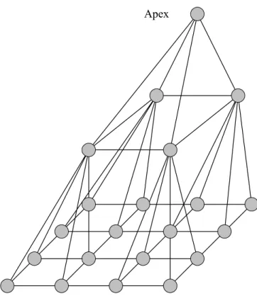
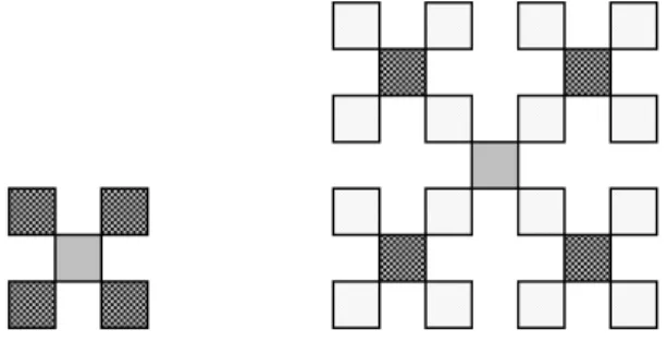
(2) current study. To date there is no proposed permutation method for a two-dimensional mesh in a pyramid structure, so in this paper we being with a Dotted Triangle as introduced by Bhattacharya and then propose a new two-dimensional embedding method to efficient implementation quadtrees and pyramids in rectangular, hexagonal or octagonal plane structures. The rest of this paper is organized as follows. Chapter 2 briefly summarizes some previous work on embedding methods, and shows the analysis and comparison after embedding. Chapter 3 discusses the different cell shapes. This paper is concluded in chapter 4. 2. Embedding Method Placement and routing are very important for efficiency and cost in VLSI layout. If we can reduce crossing and chip area using a mapping method, it will clearly increase efficiency and reduce cost. In addition, when we look for the most efficient use of the area, we must retain enough space between nodes for placement and routing. 2-1 Pyramid Architectures The pyramid is a well-known parallel network in the field of image processing and pattern recognition. Because it an extremely efficient and extensive application of interconnection structure [2,7,10,11]. Figure 2.1 shows a three- levels pyramid network. A pyramid of size n is a machine that can be viewed as a full, rooted, 4-ary tree of height log 4 n , with additional horizontal links so that each horizontal level is a mech. It is often convenient to view the pyramid as a tapering array of meshes. A pyramid of size n has a mesh of size n at its base, and a total of. 4 1 n − processors. A processor at level k is connected via bi-directional 3 3. unit-time communication links to its 9 neighbor (assuming they exist): 4 siblings at level k, 4 children at level k − 1 , and a parent at level k + 1 . The diameter of a k-level pyramid is 2k-2 and its maximum node degree is 9 for k ≥ 4 .. 2.

(3) Apex. Figure 2.1 A three-level pyramid. A pyramid network can be defined recursively, and a single node is a one-node pyramid since the single node doubles as the pyramid’s apex and its 1× 1 base. A k-level pyramid consists of a 2 k × 2 k base mesh, with group of four nodes forming 2 × 2 submeshes on the base, connected to each node of the base of a (k −1) -level pyramid.. A Pk (i, j , k ) pyramid can be viewed as consisting of a hierarchy of two-dimensional. lattices V (i, j ) through V (i ' , j ' ) , as follows [33]: A k-level pyramid Pk is a graph with vertex set. V (i, j , k ) = U {(i ' , j ' , k )(i ' , j ' ) ∈ V (i, j , k )} m. k =0. edge set. E (i, j , k ) = U {((i, j , k ), (i ' , j ' , k )) ((i, j ), (i ' , j ' )) ∈ E (M k )}U m. k =0.    a  b   ' '     ( ) ( ) ( ) ∈ a , b , k , , , k 1 i , j V M −  U k    i   j    k =1          m. 3.

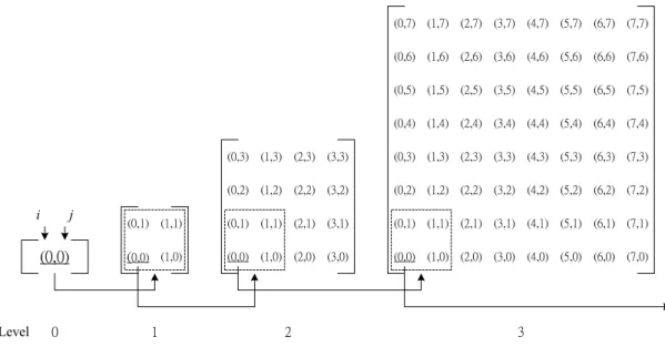
(4) (1,7) (2,7) (3,7). (4,7) (5,7). (6,7) (7,7). (0,6). (1,6) (2,6) (3,6). (4,6) (5,6). (6,6) (7,6). (0,5). (1,5) (2,5) (3,5). (4,5) (5,5). (6,5) (7,5). (0,4). (1,4) (2,4) (3,4). (4,4) (5,4). (6,4) (7,4). (0,3) (1,3). (2,3) (3,3). (0,3) (1,3) (2,3) (3,3). (4,3) (5,3). (6,3) (7,3). (0,2) (1,2). (2,2) (3,2). (0,2). (1,2) (2,2) (3,2). (4,2) (5,2). (6,2) (7,2). (0,1) (1,1). (0,1) (1,1). (2,1) (3,1). (0,1) (1,1) (2,1) (3,1). (4,1) (5,1). (6,1) (7,1). (0,0). (0,0) (1,0). (0,0) (1,0). (2,0) (3,0). (0,0). (1,0) (2,0) (3,0). (4,0) (5,0). (6,0) (7,0). 0. 1. i. Level. (0,7). j. 2. 3. Figure 2.1 A three-level pyramid. Pyramid structure combines the advantages of a two-dimensional mesh and a quadtree. The first advantage of the pyramid over the mesh is that the communication diameter of a pyramid computer of size n is only. Θ(log n) . This is true since any two processors in the pyramid. can exchange information through the apex. If too much data needs to be passed through the apex, then the apex becomes a bottleneck. Secondly, whether the pyramid is upper-lower level (Parent-Children) or on the same level (Neighbor), it have a good transmission efficient that is better than a two-dimensional mesh or a quadtree for the passage of messages. In addition, a. pyramid network has Θ( N 2 ). nodes, Θ(N ) bisection width and Θ(log N ) diameter.. In this paper we demonstrate that a radically different approach can be used to tackle the embedding problem in an array of PE’s. In our approach, a PE can be used both as a node in the graph and as a connecting element between distant nodes. We study the particular problems of the quadtree and the pyramid and show that is possible to utilize 67% of the PE’s as two-dimensional meshes. 2-2 Embedding Method Figure 2.2 shows a two level quadtree and pyramid in a two-dimensional mesh. To reduce crossing, we place the upper level in the center and the lower level surrounding the center to reduce chip area. Figure 2.3 shows a three-level quadtree and pyramid embedding in a two-dimensional mesh. This method can be used to embed more levels, although crossing in the pyramid cannot be avoided but quadtree is no cross. Figure 2.4 shows four-level quadtree structure embedding in a two-dimensional mesh. From the figure we can see there are no connections between the nodes and bring crossing, so combining two links at most we can economize on the layout cost.. 4.

(5) Figure 2.2 Quadtree and pyramid network.. Figure 2.3 A 3-level quadtree and pyramid into 2-dimensional mesh.. Figure 2.4 A four-levels quadtree.. 5.

(6) Figure 2.5 A four-levels pyramid. Figure 2.5 shows a pyramid structure embedded in a two-dimensional mesh, showing that, we can combine at most three links in a node of the same direction. It is very important to know that combining three links is constant. It will can’t increase follow extend of the pyramid. In next section, our proposal is base on three different meshes to implement quadtree and pyramid embedding in a two-dimensional mesh, and we provide an analytical comparison for every embedding and node utility. There are three kinds of meshes in Figure 2.6: rectangular-connected mesh, hexagonal-connected mesh and octagonal-connected mesh.. Figure 2.6 Three kinds meshes 2-3 Analysis and Comparisons In this section we focus on three kinds of different meshes to embed quadtrees and pyramids. 6.

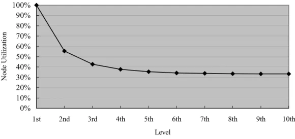
(7) in a two-dimensional mesh, and to analyze and compare utilization of the nodes. 2-3-1. Rectangular-connected mesh. Figure 2.7 Three levels quadtrees and pyramids embedding in rectangular-connected mesh. In the rectangular-connected mesh we will embed a quadtree and a pyramid in our permuted two-dimensional mesh. After the permuted show the after permutation. From the figure we obtain two different kinds of embedding, but they occupy the same nodes. Let N k be the total of number nodes for a quadtree or pyramid, and we can obtain the following general formula:. Nk =. 4k − 1 3. (2.1). Because of number of nodes will increase as the scale of quadtree or pyramid are extended, so the range that is occupied will gradually extend in the meshes. We use M kR to express the capability of a k-level quadtree or pyramid for the total number of nodes in the smallest range of rectangular mesh.. M kR = (2k − 1). 2. (2.2). From (2.1) and (2.2) we can obtain the ratio which the node occupy in a k-level qaudtree or pyramid, as follows:. 4k − 1 N rkR = kR = k 3 2 M k (2 − 1). (2.3). Where R indicates “rectangular meshes” and k indicate “levels”. We use substitution for the number in (2.3). We can obtain a curved line in figure 2.8, which grows after the seventh level as the node utility maintains about 33%. In other words about 67% will be wasted. Thus it can be seen, embedding a quadtree or pyramid base on rectangular meshes will provide a significantly lower ratio of occupied node. We obtain a 59% ratio of node occupation based. 7.

(8) Node Utilization. on Bhattacharya’s [1] scheme for the same embedding, but it is still low. 100% 90% 80% 70% 60% 50% 40% 30% 20% 10% 0% 1st. 2nd. 3rd. 4th. 5th. 6th. 7th. 8th. Level. Figure 2.8 The performance of the rectangular-connected mesh. 2-3-2. Hexagonal-connected mesh. 8. 9th. 10th.

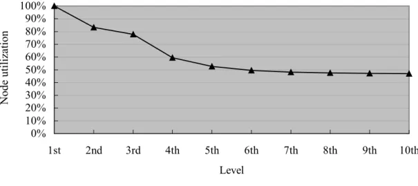
(9) Figure 2.9 No-cross approaches to embed quadtree into hexagonal meshes. In this section we provide further analysis based on hexagonal meshes after embedding to obtain the ratio of node occupation. The first to propose hexagonal meshes was Gordon [3,4] in 1982, who been embedded a binary tree in hexagonal meshes, obtaining 93% ratio of node occupation. In the current study we use a no-cross approach to embed a quadtree in a hexagonal, as in Figure 2.9. From that. figure it can be seen that need (4 × 3) + (5 × 3) nodes to cover the hexagonal meshes in the. third level and (11 × 7 ) + (11 × 6 ) nodes for the fourth level, but after the fifth level we can obtain the following general formula:. M kH = 13 × ∑ 2i−5 + 11(7 × 2i −3 − 1) i =5   k. (2.4). Where H indicates hexagonal meshes and k indicates levels. From (2.1) and (2.4) we can obtain the ratio of node occupation as follows:. 4k − 1 N 3 rkH = kH = k Mk 13 × 2i−5 + 11(7 × 2i−3 − 1)   ∑ i =5  . (2.5). Figure 2.10 is a curved line of node occupation where k ≤ 10 , and the figure maintains 47% ratio of node occupation after the eighth level. Although this approach has no crossing, but the ratio of node occupation is lower. Furthermore, we can also find unsuitable pyramid embedding in hexagonal meshes, which will cause many links to overlap and be unable to. Node utilization. connect on the same level. 100% 90% 80% 70% 60% 50% 40% 30% 20% 10% 0% 1st. 2nd. 3rd. 4th. 5th. 6th. 7th. 8th. Level. Figure 2.10 The performance of the hexagonal-connected meshes 2-3-3. Octagonal-connected mesh. 9. 9th. 10th.

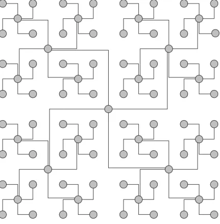
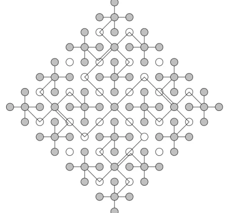
(10) In 1982 Synder [12] proposed octagonal structure, and we use this approach to design a new embedding rule. Figures 2.11 and 2.12 show a four-level quadtree and pyramid respectively embedding in an octagonal mesh graph. After a k-level quadtree and pyramid are embedded in block of octagonal meshes we can obtain the total number of node in the block as follows:. M kO = (2 k −1 ) + (2 k −1 − 1) 2. 2. (2.6). Then, taking advantage of (2.1) and (2.6) we can obtain the ratio of nodes that are occupied as follows:. 4k − 1 N rkO = kO = k −1 2 3 k −1 2 M k (2 ) + (2 − 1). (2.7). Where O indicates octagonal meshes. Figure 2.13 is substitution for the numerical calculation of (2.7). From the curved line we obtain after seven levels, the ratio of occupied nodes is 67%. This is the best ratio of occupied nodes in our proposed three approaches. When n → ∞ , then (2.7) will converge to 0.6 ≅ 0.67 , so regardless of how many levels there are, the ratio of occupied nodes will be lower than 67 percent.. Figure 2.11 A 4-level quadtree embedding in octagonal-connected meshes.. 10.

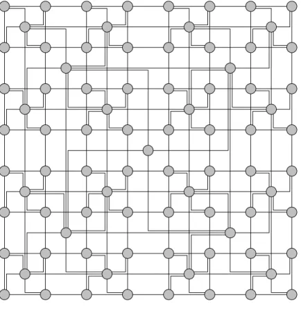
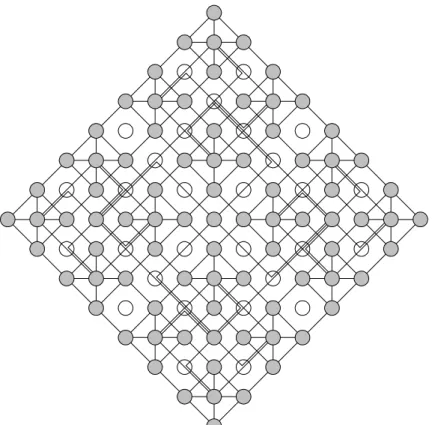
(11) Node Utilization. Figure 2.12 A 4-level pyramid embedding in octagonal-connected meshes. 100% 90% 80% 70% 60% 50% 40% 30% 20% 10% 0% 1st. 2nd. 3rd. 4th. 5th. 6th. 7th. 8th. 9th. 10th. Level. Figure 2.13 The performance of the octagonal-connected meshes. 2-3-4. Integrate comparisons. We will show the outcome in table 2.1 and figure 2.14 from the upward proof to convenient comparison. We proposed octagonal meshes embed have the best ratio of nodes occupy from the table and figure. Especially comparison with Bhattacharya’s scheme our approach obtain higher utility and without crossing problem.. 11.

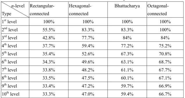
(12) In this chapter, we took the quadtree presented by Bhattacharya for instance, if the cross linkage is not considered; the eventual use rate of nodes is approximately 64%. But the quadtree embedding method presented by Bhattacharya still has cross linkage problem. Once the number of levels for cross linkage escalates, it is inevitably that the complexity of circuiting and the cost will increase. As far as the future augmentation is concerned, the complexity. of. circuiting. will. absolutely. obstruct. the. expansion.. Utilizing. the. octagonal-connected embedding method we suggest, however, can avoid the cross linkage problem, as well as the advantage over the embedding method presented by Bhattacharya in terms of the future expansion. Additionally, the 67% use rate of the nodes is remaining better than that of 64%. Table 2.1 Four kinds of embedding. n-level Type. Rectangular-. Hexagonal-. connected. connected. st. Bhattacharya. Octagonalconnected. 1 level. 100%. 100%. 100%. 100%. 2nd level. 55.5%. 83.3%. 83.3%. 100%. rd. 42.8%. 77.7%. 84%. 84%. th. 4 level. 37.7%. 59.4%. 77.2%. 75.2%. 5th level. 3 level. 35.4%. 52.6%. 67.3%. 70.8%. th. 34.3%. 49.6%. 63.1%. 68.7%. th. 7 level. 33.8%. 48.2%. 61.1%. 67.7%. 8th level. 33.5%. 47.5%. 60.1%. 67.1%. 9 level. 33.4%. 47.2%. 59.7%. 66.9%. 10th level. 33.3%. 47.0%. 59.4%. 66.7%. 6 level. Node Utilization. th. 100% 90% 80% 70% 60% 50% 40% 30% 20% 10% 0% 1st. 2nd. 3rd. 4th. 5th. 6th. 7th. 8th. 9th. Level. Rectangular. Hexagonal. 12. Bhattacharya. Octagonal. 10th.

(13) Figure 2.14 Comparison of embed. 3. Area utilization In the discussion of the previous section, the shape of a cell is shown as a circle, although actually, polygons are more common in VLSI. Since increasing the number of sides to a polygon will make masking more complicated and raise the cost of circuiting, we use squares, hexagons and octagons for discussions. In addition, the more sides a polygon has, the more complicated it is to discuss, which will also increase the difficulty of production. Figures 3.1, 3.3 and 3.5 represent square, hexagonal and octagonal 3-level quadtree networks, respectively. Figure3.7 and Table 3.1 show the comparison of cells’ actually occupied area with the whole area of the chip. We can obtain from this curve the use rate of each polygon. Next, we analyze the use rate of the areas of squares, hexagons and octagons. 3-1 Square Node In the square, as shown in figure 3.1, we assume the area of each node to be 1, the number of nodes of the k-levels to be. 4k − 1 ，and the area of the k-level of cell in the square to be: 3  4 − 1   3  R  αk = k (2 − 1)2 k. (3.1). Using numerical values for substitution, the results are shown in Figure 3.2. We can obtain from this curve that, although there is no technical problem in the square, the use rate of the area is relatively low. Since the use rate of the area is only 33% after the 7th level, therefore we do not use this method.. Figure 3.1 Square layouts.. 13.

(14) Area Utilization. 100% 90% 80% 70% 60% 50% 40% 30% 20% 10% 0% 1st. 2nd. 3rd. 4th. 5th. 6th. 7th. 8th. 9th. 10th. Level. Figure 3.2 Area utilization of the square. 3-2 Hexagon Node For the hexagon, as shown in figure 3.3, we obtain the area of the hexagon in a square whose unit area is 1 as 0.75. The area of the nth level of cell in the hexagon is 5   k −3   k + × 5 6   ∑ (2 )  × 2  α kH =   k =3 4. (3.2). Using numerical values for substitution, results in the curve shown in Figure 3.4. We can obtain this figure that the hexagon has an area use rate of about 66%, but there is no room for circling lines between nodes, which will obstruct the transmission of messages between nodes. This situation will result in an extra level to be administered for transmitting messages, which will increase the cost of circuiting; therefore we do not adopt this method.. Figure 3.3 Hexagon layouts.. 14.

(15) Area Utilization. 100% 90% 80% 70% 60% 50% 40% 30% 20% 10% 0% 1st. 2nd. 3rd. 4th. 5th. 6th. 7th. 8th. 9th. 10th. Level. figure 3.4 Area utilization of the hexagon 3-3 Octagon Node. In the octagon, as shown in figure 3.5, we obtain the area of the octagon in the unit area as. 7 = 0.7 . The area of the k-levels of cell in the octagon is 9 7  4k − 1    9 3  O αk = 2 1 k i 2  ∑   3 i =0 . (3.3). Using numerical values for substitution results in the curve shown in Figure 3.6. The octagon has an area use rate of about 58%. Although the effective use rate of the area is lower than that of hexagon, the room between nodes can be used for circuiting. Thus it will achieve a better degree of efficiency coordinating with the octagonal-connected embedding method we present. Next, we will show the changes of area when the number of levels of the quadtree or the pyramid is approaching infinitely large number.. Figure 3.5 Octagon layouts.. 15.

(16) Area Utilization. 100% 90% 80% 70% 60% 50% 40% 30% 20% 10% 1st. 2nd. 3rd. 4th. 5th. 6th. 7th. 8th. 9th. 10th. Level. Figure 3.6 Area utilization of the octagon. When the number of levels n → ∞ ，we can have the following equation:.  7  4k − 1       9  3 2  lim k →∞  1 k i   2   3 ∑   i =0   and 2.  2i  = (2k +1 − 1)2 = 22 k +2 − 2 ⋅ 2k +1 + 1 ∑   i =0  therefore the original equation = k. 7 1 22 k − 1 × × 9 × lim k →∞ 9 3 22 k +2 − 2k +2 + 1 = 0.583 The values we use here are the same as the results that we substitute after the 7th level. Therefore we can prove that when the number of levels is high, the quadtree or the pyramid still retains a 58% area use rate, so area will not be waste because of the increasing number of levels. We can obtain from table 3.1 that the occupied area is approaches 33% for the square, 66% for the hexagon, and 58% for the octagon. Table 3.1 Three kinds of cell shapes. Level. 1st. 2nd. 3rd. 4th. 5th. 6th. 7th. 8th. 9th. 10th. Shape Rectangula 1.0000 0.5555 0.4285 0.3777 0.3548 0.3439 0.3385 0.3359 0.3346 0.3339 r Hexagonal 0.7500 0.7500 0.7159 0.6929 0.6801 0.6735 0.6701 0.6683 0.6675 0.6671 Octagonal 0.7777 0.7142 0.6533 0.6191 0.6014 0.5924 0.5878 0.5856 0.5844 0.5839 3-4 Integrate Comparisons 16.

(17) Concluding from the figures and tables above, we make the following analysis: 1. The space of the square cell has big gap, which is easy to circuit. But this big gap wastes more space, resulting the most wasted area of the chips among the 3 methods. 2. The space of the hexagon cell has the smallest gap, so it has the best arrangement of the space. But many cells are tightly connected, which obstructs the actual circuiting and results in inconvenience. 3. The arrangement of the space of the octagon is not as tight as that of the hexagon, but there is enough room left for circuiting between each cell, and it particular every side is used to connect neighboring nodes, which is the most interesting aspect of this method.. Figures 3.7 and 3.8 are examples of a 4-level (8 × 8) quadtree network and pyramid. network. We first rotate the above-mentioned octagonal-connected embedding method 45 degrees, and then use the array shown in Figure 3.9, so every cell is presented as an octagon. In order to decrease the area and save the space, every cell is tightly connected.. Figure 3.7 The quadtree network of octagon.. 17.

(18) Node Utilization. Figure 3.8 The pyramid network of octagon.. 100% 90% 80% 70% 60% 50% 40% 30% 20% 10% 0% 1st. 2nd. 3rd. 4th. 5th. 6th. 7th. 8th. 9th. 10th. Level Rectangular. Hexagonal. Octagonal. Figure 3.9 Three kinds of area utilization based on various cell shapes. Conclusions. In this paper, we propose detailed discussion of quadtrees and pyramids embedded in two-dimensional meshes and the VLSI layout. We propose three different mapping and illustrate how to embed a three-dimensional architecture in two-dimensional meshes. We also determine the ratio of occupied nodes in every embedding method. Furthermore, we also calculate the polygons for every cell. We obtain higher node utility base using octagonal. 18.

(19) meshes in two-dimensional embedding, and higher area utilization based on octagon cells. In this approach, it is helpful to reduce the complexity of layout in VLSI arrays. This does not affect the scale of the array, and it maintains efficient utilization of chip area. References. [1] Battacharya, S., S. Kriani, and W. T. Tsai, “Quadtree Interconnection Network Layout,“ Proceedings of the Second Great Lakes Symposium on VLSI, pp.81-87, 1991. [2] Codenotti, B. and M. Leoncini, Introduction to Parallel Processing. Addison-Wesley, 1993. [3] Gordan, D., I. Koren, and G. M. Silberman, “Embedding Tree Structures in VLSI Hexagonal Arrays,” IEEE Trans. Computer, Vol. C-33, no. 1, pp.104-107, 1984. [4] Gordan, D., “Efficient Embeddings of Binary Tree in VLSI Arrays,” IEEE Trans. Computer, Vol. C-36, pp.1009-1018. Sept. 1987.. [5] Ho, C.-T., and S. Lennart Johnsson., “Dilation d Embedding of a Hyper-pyramid into a hypercube,” Proceedings of the Supercomputing Conference, pp.294-303, 1989. [6] Kumar, V. K. P and D. Reisis., “Pyramids versus Enhanced Arrays for Parallel Image Processing,” Technical Report CRI-86-16, Department of Electrical Engineering-Systems, 1986, University of Southern California. [7] Leighton, F. T., Introduction to Parallel Algorithms and Architectures. Morgon Kaufmann, 1992. [8] Mead, C. and L. Conway, Introduction to VLSI System. Addision-Wesley, 1980. [9] Nandy, S. K. and I. V. Ramakrishnan, “Dual Quadtree Representation for VLSI Designs,” Proceedings of the 23th Design Automation Conference, pp.663-666, 1986. [10] Suaya, R. and G. M. Birtwustle, VLSI and Parallel Computation. Morgan Kaufmann, 1990. [11] Samet, H., “The Quadtree and Related Hierarchical Data Structures,” ACM Computing Survey, Vol. 16, pp.187-260, 1984.. [12] Snyder, L., “Introduction to the Configurable Highly Parallel Computer,” IEEE Computer, pp.47-64, Jan. 1982.. 19.

(20)