技術面選股分析

國立交通大學

管 理 學 院

企業管理碩士學位學程

碩士論文

技術面選股分析

The Analysis of Technical Trading Strategies:

Using Technical Indicators Sharpe Ratio and MACD on Selected S&P 500 Stocks

研究生：張丹

指導教授：劉助

The analysis of technical trading strategies:

Using technical indicators Sharpe ratio and MACD on selected S&P 500 stocks

研究生：張丹

指導教授：劉助

國立交通大學

管理學院

企業管理碩士學位學程

碩士論文

A Thesis

Submitted to Master Degree Program of Global Business Administration College of Management

National Chiao Tung University In Partial Fulfillment of the Requirements

For the Degree of Master

in

Business Administration June 2014

Hsinchu, Taiwan, Republic of China

Abstract

Background: Interest in investing in the stock market has grown in recent years,

with a greater number of non-specialists trying to balance risk and return. Although they are popular, most people at best only have a basic understanding of how stocks work, even though the risks involved require scientific knowledge. Any investor who has knowledge of the principles and analytical methods involved in portfolio management has a greater chance of success.

Objectives: This thesis focuses on the role of technical analysis in passive

management of portfolio and in signaling the timing of the stock market entry. This thesis studies the profitability of applying technical analysis indicators Sharpe Ratio and MACD on the top of the fundamental based strategy called "Quality Based Investing Strategy".

Results: Using companies listed in S&P 500, the results indicates that especially one

of the proposed technical strategies called Sharpe 130 can be used to generate significantly positive return and outperform strategy solely based on fundamental analysis and also buy and hold strategy of underlying S&P 500 index in most cases.

Conclusion: In conclusion it has been shown that investors can benefit by having

investment strategies utilizing both fundamental and technical analysis

Acknowledgements

I would like to express my sincere gratitude to my supervisor, Dr James Liu for providing a very supportive environment throughout the thesis writing process, and who has supported me with his patience and knowledge. He often went above and beyond what was required of him lending help to students. He introduced me to stock trading which I become personally interested in ever since. Thanks to his guidance and supervision Prof. Liu has definitely deepened my interest in research. Having an advisor like him is truly an inspiration and motivation for any student.

My sincere thanks also belong to other professors and teaching assistants for their valuable comments, suggestions and advice during our seminars.

Table of Contents

Abstract ... i 

Acknowledgements ... ii 

Table of Contents ... iii 

List of Tables ... v 

List of Figures ... vi 

Section 1: Introduction ... 1 

Objective of Study ... 3 

Section 2: Theory and Literature Review ... 4 

Technical Analysis ... 4 

Technical Analysis and the Abnormal Return ... 4 

Technical Analysis and Trends and Timing ... 6 

Portfolio Theories ... 7 

Portfolio Analysis Research ... 7 

Section 3: Research Methodology ... 9 

Technical Indicators ... 9 

Sharpe Ratio ... 9 

MACD ... 10 

Default Research Framework ... 12 

Dataset ... 12 

Methodology restriction rules ... 13 

Methodology Number 1. (Stacking up of Portfolios) ... 14 

Methodology Number 2. (Swapping the Portfolios) ... 15 

Sharpe ratio criterion ... 18 

Sharpe 260 ... 18  Sharpe 130 ... 18  MACD criterion ... 19  Holding period ... 20  Return rates ... 20  Section 4: Results ... 21 

Methodology number 1. (Stacking up of portfolios) ... 21 

Methodology number 2. (Swapping the portfolios) ... 23 

Section 5: Conclusion ... 25 

Study Limitations and Recommendation for Future Work ... 27 

References ... 28  Appendix 1 ... 30  Appendix 2 ... 31  Appendix 3 ... 32  Appendix 4 ... 33  Autobiography ... 34 

List of Tables

Table 1 Research design methodology number 1 ...15 Table 2 Research design methodology number 2...16 Table 3 Results of methodology number 1.Cumulative return rates of proposed technical strategies and benchmarks fundamental strategy and S&P 500 index...21 Table 4 Results of methodology number 2.Cumulative return rates of proposed technical strategies and benchmarks fundamental strategy and S&P 500 index...23 Table 5 Stocks according tic symbols included in portfolios constructed on the basis of fundamental methodology "Quality investing strategy" (Buranovsky, 2014) ...30

List of Figures

Figure 1 Compound return of technical strategies by methodology number 1...22 Figure 2 Compound return of technical strategies by methodology number 2...24 Figure 3 List of the companies according investing strategies based on technical

analysis...31 Figure 4 Sample of MACD computations...32 Figure 5 Sample of Sharpe 260 and Sharpe 130 computations...32 Figure 6 Yearly (Y) and Cumulative (C) return rates according each investing strategy of each portfolio - Methodology number 1 ...33

It’s far better to buy a wonderful company at a fair price than a fair company at a wonderful price.

-Warren Buffet

Section 1: Introduction

Over the last few decades, the average person's interest in the stock market has grown exponentially. What was once exclusive to rich individuals and institutions has now turned into the vehicle of choice for the growing wealth for retail investors. This demand, coupled with advances in trading technology, has opened up the markets so that nowadays nearly anybody can own stocks. Despite their popularity however, most people do not fully understand stocks, and the great deal of risk associated with investing calls for a scientific knowledge. An investor who understands principles and analytical aspects of portfolio management has a better chance of success.

There are essentially two ways used to analyze stocks (or any other type of securities) and make investment decisions: fundamental and technical analysis. With the former, the investor aims to determine the value of the company by analyzing its financial statements, its management and competitive advantages, and its competitors and markets. Also factors pertaining to overall state of the economy are often considered in

fundamental analysis. In contrast, technical analysis studies supply and demand in a market, in an attempt to recognize prevailing "sentiment" and determine what direction, or trend, will continue in the future. Considering the difference in the underlying

for the large part, the literature is (understandably) divided for research purposes along this synopsis, which only confirms the belief that fundamental and technical analysis are polar opposites.

However, in real world trading, especially considering long-term investing time frame, it is quite popular to combine the tools offered by both methods, and approach which can help investors better understand the markets and gauge the direction in which their investments might be headed. For instance, fundamental analysis may play an important role during the process of selecting securities, and technical analysis becomes useful in timing individual trades and organizing portfolios according investors

risk/return ratio preferences. The moral of the story is that technical analysis and

fundamental analysis are not warring factions, but nor are they contradictory philosophies. The two can be used in unison to find winning stock ideas. Combination of the two with a sound risk management strategy may lead to many profitable days in the market.

This thesis is organized as follows: In the next section I review the related theories and literature. In the first part, I generally describe technical analysis and describe the relationship pertaining to technical analysis and abnormal returns, and technical analysis and timing and trends. In the final part of the literature review I introduce the portfolio theory concept. In Section 3, a description of technical indicator MACD and Sharpe Ratio is provided. In this part, I also describe the methodology of this research. I introduce, and provide an overview of, the research design. This section also includes a description of Sharpe ration and MACD criteria. I present the results in comparison to the "Quality based investing strategy" and also to the performance of a

benchmark index. In the final part of the thesis I discuss the results and its implication on real world trading.

Objective of Study

 To analyze predictability of return rate using technical analysis tools: Sharpe Ratio and MACD

 To analyze results and compare them with return rate of plain portfolio designed through fundamental analysis

 To analyze whether the Sharpe Ratio, MACD, or a combination of methods, can inform the “average” investor (non-specialists) about which stocks will make gains.

Section 2: Theory and Literature Review

Technical Analysis

According to the philosophy of technical analysis, prices of securities (stocks, bonds, commodities, and so on) are determined by demand and supply forces operating in the market. These demand and supply forces are, in turn, influenced by a number of fundamental (economic, monetary, and political) factors, as well as certain psychological or emotional factors. The combined impact of all these factors can be reduced to a single variable: market price.

The technical analysts (also known as chartists) believe that securities prices move in trends and that those trends repeat themselves over time. Therefore, the historical price and volume movements of stocks and markets are indications of future performance. Based on this premise, they study the price and volume movements in the market and try to find patterns in them. While some indicators use complex formulas and others are more simple, all of them seek to establish visual patterns that make sometimes confusing price data easier to understand and interpret. Indicators can be applied to stock, indexes, futures contracts and any other tradable instruments whose prices move in response to the influence of supply and demand.

Technical Analysis and the Abnormal Return

Since Charles H. Dow first introduced the Dow Theory in the late 1800s, technical analysis has become matter of controversy. In practice, many practitioners (brokers, fund managers, investors, and so on) attribute a significant role to technical

analysis. Taylor and Allen (1992) report the results of a survey among chief foreign exchange dealers based in London in November 1988, and found that at least 90 percent of respondents placed some weight on technical analysis. This has been echoed by Schwager (2012) who interviewed top traders and fund managers and found that many top traders and fund managers use some form of technical analysis extensively.

However, despite its widespread acceptance and adoption by practitioners, academics have, on the other hand, long been skeptical about usefulness of technical analysis. Some empirical studies (Fama and Blume 1966, Jensen and Benington 1970 and Fong and Yong 2005) do not see any merit in technical analysis. Rather, they tend to believe that markets are informationally efficient and hence all available information is impounded in current prices so, no abnormal returns can be made with historical price and other market data. (Fama 1970).

Although these studies are not in favor of technical trading rules, there are also findings showing the opposite. Treynor and Ferguson (1985) argued that when the non-price information is taken into account, historical non-prices can help to generate higher returns. Brock et al. (1992) analyzed 26 technical trading rules using 90 years of daily stock prices from the Dow Jones Industrial Average up to 1987, and found that they all outperformed the buy-and-hold strategy. Mills (1997) showed a similar result for the FT30 index. Kwon and Kish (2002) reported that the technical rules beat the buy-and-hold strategy in the NYSE.

Technical Analysis and Trends and Timing

The use of market timing has long been a subject of much discussion, because usually there is little or no consensus through the research studies as to whether

techniques such as moving averages can produce better returns than buy and hold strategy. Among those who tested the MACD indicator are Brock, Lakonishok and

LeBaron (1992), who tested several moving averages and found them useful in predicting stock prices. However, their benchmark was merely holding cash. Seyoka (1991) tested the MACD indicator from 1989 to 1991 on the S&P 500. His results questioned the indicators’ usefulness. Sullivan, Timmermann and White (1999) found superior

performance of moving averages for the Dow Jones Industrial Average for in-sample data. However, their results showed no evidence of outperformance for out-of-sample data.

As studies are indicating the main shortcomings of trading based on moving averages such as MACD, are the whipsaws effect and the costs of transactions associated with it. Whipsaws effect means generating several transactions based on false signals due to short lived changes in direction. Traders can get whipsawed in and out of a position several times before being able to capture a strong change in momentum. When the cost of transactions are factored into the equation, this strategy can become very expensive.

However, in this research MACD is utilized not as a standalone trading strategy i.e. trading on buy and sell signals generated by MACD as researchers mentioned above have done, but only as an extension of buy and hold strategy, where MACD will be only functioning as trigger for one buy signal at the beginning. Only the first buy signal for respective companies within the study period will be taken into consideration. Therefore, neither account transaction costs, or whipsaw effect are taken into account.

Portfolio Theories

The fundamental question in finance (investing) is how the risk of an investment should affect its expected return; does more risk guarantee higher returns? To mitigate some of the risk, it is often advisable to diversify one's holdings in an investment portfolio. A portfolio is a group of securities held together as investment. By spreading the investment across a number securities, the risk of achieving low returns, or worse, losing money, is reduced. Naturally, there is always risk involved, but security analysis allows the risk-return characteristics of each security to be quantitatively measured, and investment portfolios to be put together that provide the highest returns for a level of risk that is acceptable to each investor.

Portfolio Analysis Research

Markowitz (1959) was the first to show that proper risk reduction through proper diversification required the building of investment portfolios. This established Modern Portfolio Theory, which was extended further by Sharpe (1966). Sharpe's portfolio performance ratio of expected return to its standard deviation, known as the Sharpe ratio is widely used and cited in the literature and pedagogy of finance. Although it is popular, the Sharpe Ratio does have a methodological weakness in that it relies on normally distributed returns as a measure. If returns not normally distributed, the Sharpe ratio is arguably, a much less accurate measure as abnormalities like kurtosis, fatter tails and higher peaks, or skewness are not taken into account.

This limitation of the Sharpe ratio has not gone unnoticed in the literature. In fact, this issue of non-symmetrical distributions has motivated the development of numerous new performance measures, including the Omega ratio (Keating and Shadwick, 2002), the Sortino ratio (Rom, 1983), the Calmar ratio (Young, 1991), and the modified Sharpe ratio (Sharpe, 1994). However, Eling and Schuhmacher (2007) compared the Sharpe ratio with 12 other approaches to performance measurement. They focused on the returns of 2,763 hedge funds. Despite hedge fund returns’ significant deviation from a normal distribution, the Sharpe ratio and the other measures result in virtually identical rank ordering across the hedge funds. In other words, the choice of performance measure did not matter much in terms of ranking funds. From a practical perspective, this imparts credibility to the use of the Sharpe ratio for ranking funds with highly non-normal returns. In conclusion, the accuracy of Sharpe ratio estimators hinges on the statistical properties of returns, and these properties can vary considerably among strategies, portfolios, and over time. Also, investors should also keep in mind that the Sharpe ratio is calculated using past performance, meaning it offers no guarantee on how a fund might behave in the future. Despite such caveats, for a number of investment decisions, Sharpe Ratios can provide important inputs. When used in conjunction with other measures, the Sharpe ratio can help investors develop a strategy that matches both their return needs and risk

Section 3: Research Methodology

Technical Indicators Sharpe Ratio

This risk-adjusted measure was developed and introduced by Nobel Laureate William Sharpe in 1966. It is calculated by using standard deviation and excess return to determine reward per unit of risk. Sharpe ratio is a popular for its simplicity as a

relatively quick and easy way to examine the performance of an investment by adjusting for its risk. The higher a fund's Sharpe ratio, the better its returns have been relative to the amount of investment risk it has taken. The Sharpe ratio can be used to compare directly how much risk two funds each had to bear to earn excess return over the risk-free rate. Because it uses standard deviation, the Sharpe ratio can be used to compare risk-adjusted returns across all fund categories. Expressed in its usual form, the Sharpe ratio can be broken down into just three components: asset return, risk-free return and standard deviation of return.

Sharpe ratio formula:

Return (rx) is what a fund returned over a set period and subtracts risk-free (Rf)

rate of return that is, what an investor could have earned in a risk-free investment. The denominator is the fund's standard deviation (σx)which measures how much a fund strays

MACD

MACD (Moving Average Convergence Divergence), is a trading indicator used in technical analysis of stock price and trends. It was devised by Gerald Appel in the late 1970s. It is supposed to reveal changes in the strength, direction, momentum, and duration of a trend in a stock's price. The indicator has been applied by many traders across all types of markets, because it is seen as simple and intuitive, and is in common use today.

The MACD indicator depends on three time parameters, namely the time constants of the three exponential moving averages (EMAs). These are used instead of simple moving averages, because EMA's are calculated to reflect prices over a stated period but emphasize more recent values.

MACD is constructed by subtracting a longer (26 days) from a shorter (12 days) moving average. This generated difference can be plotted by itself below the price chart. The resulting plot forms a line that oscillates above and below zero, without (theoretically) any upper or lower limits. In addition to the MACD, the oscillator chart includes two other plots. One is a signal line, which is plotted alongside to act as a trigger line; the other is a histogram, which is just a visual aid indicating how far is the oscillator is from signal line.

The notation "MACD (a,b,c)" usually denotes the indicator where the MACD series is the difference of EMAs with characteristic times a and b, and the average series is an EMA of the MACD series with characteristic time, c. This research uses the most popular indicator model, MACD (26,12,9). This means that numbers in following

formula stand for the number of days considered for calculation of respective exponential moving averages.

MACD formula:

The n-day EMA at a time t used in determining the aforementioned indicator is

derived from the following equation:

, 1

where

(n: number of days)

A fast EMA responds more quickly than a slow EMA to recent changes in a stock's price. By comparing EMAs of different periods, the MACD series can indicate changes in the trend of a stock. It is claimed that the divergence series can reveal subtle shifts in the stock's trend. Since the MACD is based on moving averages, it is inherently a lagging indicator. As a metric of price trends, the MACD is less useful for stocks that

Default Research Framework

This analysis is built on a previous work of Martin Buranovsky. For the technical analysis, portfolios designed by Buranovsky in his thesis "Quality Based Investing

Strategy: Investing Based on Fundamentals" (2014) were adopted as a basic framework.

Each year between 2004 and 2013 Buranovsky analyzed S&P 500 companies by using self-designed performance criteria to identify "high quality" companies for inclusion in investment portfolios. Only companies which satisfied all three criteria (Criterion 1: Cash position, Criterion 2: Growth, and Criteria 3: Profitability) were included in portfolio for each respective year. Through this selection process, Buranovsky designed 10 portfolios between 2004 and 2013. For the purpose of this research, perform technical analysis on 6 consecutive portfolios from 2008 to 2013 was chosen. The list of companies included in these 6 portfolios is given in Appendix 1.

Dataset

The daily closing prices of S&P 500 companies from March 2007 to March 2014 were obtained from COMPUSTAT, accessed through Wharton Research Data Services. All computations have been carried out using the MS Office Excel 2007 spreadsheet program.

Methodology restriction rules

In order to increase measurability and simplicity, two constraints have been imposed in this research.

Rule number 1

Since the companies were drawn to portfolios from current S&P 500 lists for each respective year (so, for example portfolio 2008 was created from the list of companies included in S&P 500 current as of March 2008) the consistency of the portfolios was checked to ensure companies listed in portfolios still exist under its tic symbol at the "present day". "Present day" in this context is the date of 28th of March 2014 which, is the last day of study period in this research. Those companies which have become defunct by 3/28/2014 are excluded from all portfolios on an ex-post basis. This way, the list of the companies included in each portfolio is fixed for entire study period.

Rule number 2

While calculating Sharpe ratios 260 days and 130 days, for simplicity it was assumed that the risk free rate is 0%. Another reason for excluding the risk free rate is that for purposes of this research there is no need to know the absolute value of Sharpe ratio for each company. Since including risk free would have been constant for every company, excluding it does not affect the ranking.

Research Design

There are 2 methodologies used to measure the performance of technical

indicators. In following part, the difference between the two methods of analysis will be explained.

Methodology number 1 imitates a situation when an investor creates, each year, a new portfolio (for each technical method) but will also keep previous ones. So, the number of portfolios will increase each year by one. In year six he will have six portfolios and will measure the performance of each of them according to each technical strategy.

Methodology number 2 imitates a situation when an investor, each year, creates a new portfolio (for each technical method), keeps it for one year and measure its performance. However, each new year he will swap the portfolio with the newly created one, which means that at any point he will hold only one portfolio.

Methodology Number 1. (Stacking up of Portfolios)

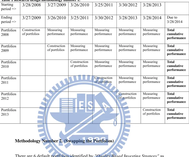
There are 6 default portfolios identified by "Quality Based Investing Strategy" as the subject of this study. Starting from 3/28/2008 with portfolio 2008, each year a portfolio is a subject to the application of technical analysis (see below in Table 1). Performance of each portfolio is further measured yearly until the last day of study period which, is 3/28/2014. Cumulative performance of each portfolio is benchmarked against the performance of fundamental method "Quality based investing strategy", and also against S&P 500 index performance for respective years. Each company in the portfolio is equally weighted.

Table 1 Research design methodology number 1. Starting period => 3/28/2008 3/27/2009 3/26/2010 3/25/2011 3/30/2012 3/28/2013 Ending period => 3/27/2009 3/26/2010 3/25/2011 3/30/2012 3/28/2013 3/28/2014 Due to 3/28/2014 Portfolios 2008 Construction

of portfolios Measuring performance Measuring performance Measuring performance Measuring performance Measuring performance Total cumulative performance Portfolios

2009

Construction

of portfolios Measuring performance Measuring performance Measuring performance Measuring performance Total cumulative performance Portfolios

2010

Construction

of portfolios Measuring performance Measuring performance Measuring performance Total cumulative performance Portfolios

2011

Construction

of portfolios Measuring performance Measuring performance Total cumulative performance Portfolios 2012 Construction of portfolios Measuring performance Total cumulative performance Portfolios 2013 Construction

of portfolios Total cumulative performance

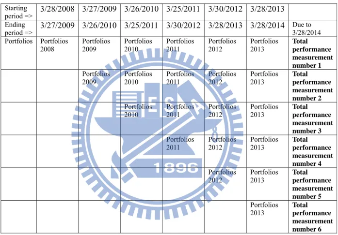
Methodology Number 2. (Swapping the Portfolios)

There are 6 default portfolios identified by "Quality Based Investing Strategy" as the subject of this study. Starting from 3/28/2008 with portfolio 2008, a portfolio subject to the application of technical analysis and performance of each technical strategy is measured at the end of yearly holding period, due 3/27/2009. Next year, new set of portfolios for each technical strategy is created in similar fashion, then it is measured and swapped for another one, and so on. (see below in Table 2) After construction of the portfolios, the cumulative performance is measured in way so that the oldest portfolio is

portfolio, 2013, is measured by itself. Cumulative performance of this strategy is benchmarked against the performance of fundamental method "Quality based investing

strategy", and also against S&P 500 index performance for respective years.

Table 2 Research design methodology number 2

Starting period => 3/28/2008 3/27/2009 3/26/2010 3/25/2011 3/30/2012 3/28/2013 Ending period => 3/27/2009 3/26/2010 3/25/2011 3/30/2012 3/28/2013 3/28/2014 Due to 3/28/2014 Portfolios Portfolios 2008 Portfolios 2009 Portfolios 2010 Portfolios 2011 Portfolios 2012 Portfolios 2013 Total performance measurement number 1 Portfolios 2009 Portfolios 2010 Portfolios 2011 Portfolios 2012 Portfolios 2013 Total performance measurement number 2 Portfolios 2010 Portfolios 2011 Portfolios 2012 Portfolios 2013 Total performance measurement number 3 Portfolios 2011 Portfolios 2012 Portfolios 2013 Total performance measurement number 4 Portfolios 2012 Portfolios 2013 Total performance measurement number 5 Portfolios 2013 Total performance measurement number 6

For each portfolio, 3 different computations have been done to create technical strategies. That is calculation of Sharpe Ratio 260 days (hereafter Sharpe 260), Sharpe

Ratio 130 days (hereafter Sharpe 130) and MACD. These 3 computations are the

resulting of 4 different observed technical strategies. In other words, from each default fundamental portfolio four different portfolios based on technical analysis with different characteristics were created:

1. Technical strategy: Sharpe 260

2. Technical strategy: Sharpe 130

3. Technical strategy: Sharpe 260 + MACD

4. Technical strategy: Sharpe 130 + MACD

For each of the four subsequent portfolio created based upon these technical indicators. Portfolio performance was calculated, and benchmarked against the

performance of fundamental method "Quality based investing strategy" and also against S&P 500 index performance for respective years.

Sharpe ratio criterion Sharpe 260

From daily closing prices, the return rate was calculated on a daily basis. That is, over period of 260 days, the daily differential returns from closing price for each stock in the portfolio were calculated. Standard functions were then utilized to compute the components of the ratio. For example, if the differential returns were in cells B1 through B260, a formula would provide the Sharpe Ratio using Microsoft's Excel spreadsheet program:

AVERAGE(B1:B260)/STDEV(B1:B260)

In other words, for default portfolio 2008 with starting period 3/28/2008, the Sharpe ratio from the 260 preceding days, that is from 3/16/2007 to 3/28/2008, was calculated. After calculating the value of the Sharpe ratio for each company in the portfolio, these companies were ranked from highest Sharpe ratio value to lowest. This way, a Top 10 list which subsequently became the new portfolio according this criterion, was created (See the table in appendix 2 for list of the companies).

Sharpe 130

Calculated in a similar fashion with consideration of 130 days prior to the beginning of the holding period. For example, for Portfolio 2008 Sharpe ratio from 9/21/2007 to 3/28/2008 was calculated.

MACD criterion

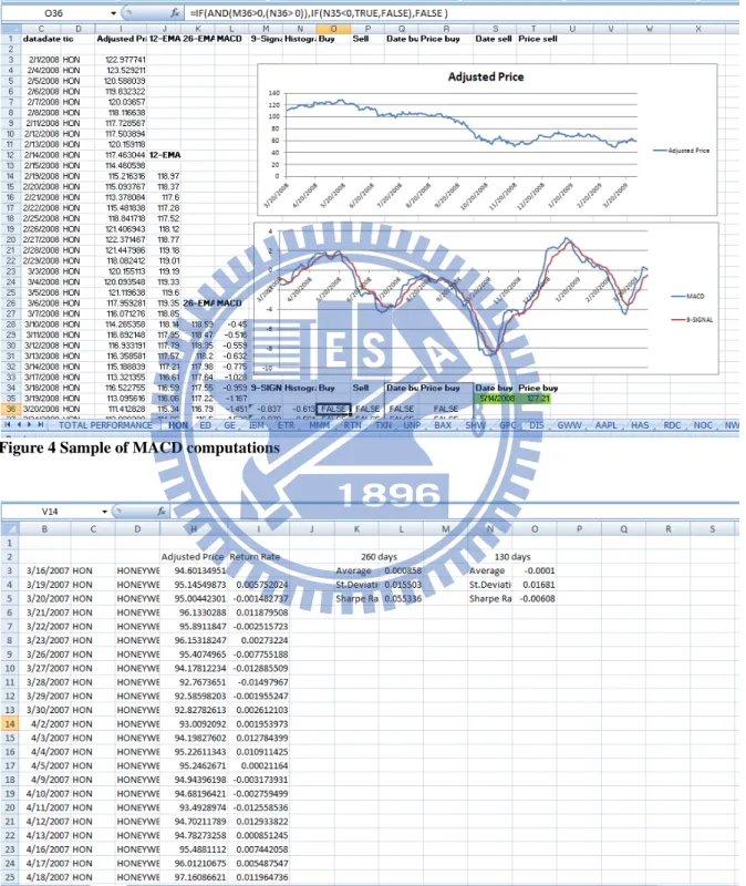
By using MACD as another technical analysis tool the aspect of timing is added into any trading strategy. However, in the described research MACD is not used in its usual way whereby investors are purchasing and selling stocks according to buy (long position) and sell (short position) signals being emitted by MACD. In this research, only the first ever buy signal occurred in designated period of time for each stock within TOP 10 list identified by Sharpe 260/ Sharpe 130 criterion is taken into consideration. The intention is to buy a stock at "right time" meaning at relatively low price before the stock gains the momentum.

The buy signal is triggered when 2 conditions are met:

1. MACD is crossing its signal line from below

2. This crossover is occurring in positive area, that is, above the zero line

For example, in Portfolio 2008 MACD is calculated using closing prices for each company from given Sharpe TOP ten subset lists and identified buy signals within the 2008 Portfolio holding period, that is within 3/28/2008 to 3/27/2009. Date and associated price of company has been identified by buy signal and used to calculate return rate between the day of purchase and the date at the end of holding period.

Holding period

In order to maintain compatibility with benchmark portfolio for comparison purposes, the analysis in this research accepts the same dates outlined by Buranovsky in his work. That is, always starting on the first Friday in March of a particular year and ending on the last Friday in March of a subsequent year. This time period is defined this way to be in more accurate compliance with the release of companies' financial

statements which are usually occurs in March.

Return rates

In order to calculate return rates of each portfolio, return rates for each company are calculated first, and then I quantify arithmetic average from all companies within one portfolio.

Following formula has been used to adjust prices form COMPUSTAT for stock splits and dividends.

ADJUSTED PRICE = (PRCCD -- Price - Close – Daily) / (AJEXDI -- Adjustment Factor (Issue)-Cumulative by Ex-Date) * (TRFD -- Daily Total Return Factor).

Section 4: Results

Methodology number 1. (Stacking up of portfolios)

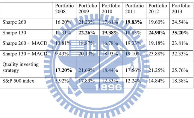
Table 3 Results of methodology number 1.Cumulative return rates of proposed technical strategies and benchmarks fundamental strategy and S&P 500 index

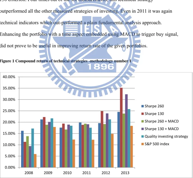
In Table 3 , the summary for the each proposed trading strategy for period from 2008 to 2014 is presented. The summary contains cumulative return rates for respective portfolios and trading strategies.

The summary indicates that the best performance for portfolio constructed in 2008 is achieved by pure fundamental analysis without applying technical indicators. The

Portfolio

2008 Portfolio 2009 Portfolio 2010 Portfolio 2011 Portfolio 2012 Portfolio 2013 Sharpe 260 16.20% 21.23% 17.61% 19.83% 19.60% 24.54% Sharpe 130 11.31% 22.26% 19.38% 18.83% 24.90% 35.20% Sharpe 260 + MACD 13.81% 18.87% 16.78% 19.33% 19.18% 23.81% Sharpe 130 + MACD 9.43% 20.13% 18.93% 19.10% 23.88% 32.33% Quality investing strategy 17.20% 21.69% 18.44% 17.56% 21.25% 25.76% S&P 500 index 5.92% 17.89% 12.33% 12.24% 14.84% 18.38%

experienced a sharp drop in 2008 but were recovering fast in the following year have been penalized due to that volatility swing and therefore, did not make it into TOP 10 list by Sharpe ratio; even though these companies have eventually enjoyed extraordinary growth in 2009 and 2010. In other words, Sharpe ratio is favoring conservative companies with the least volatility whether it is negative or positive.

For the rest of the study period, between 2009 and 2013, Table shows quite unambiguously that the best overall results are achieved by incorporating plain Sharpe 130 criterion. Four times out of the six measurements, this technical strategy

outperformed all the other measured strategies of investing. Even in 2011 it was again technical indicators which out-performed a plain fundamental analysis approach.

Enhancing the portfolio with a time aspect embedded using MACD to trigger buy signal, did not prove to be useful in improving return rate of the given portfolios.

Figure 1 Compound return of technical strategies -methodology number 1

0.00% 5.00% 10.00% 15.00% 20.00% 25.00% 30.00% 35.00% 40.00% 2008 2009 2010 2011 2012 2013 Sharpe 260 Sharpe 130 Sharpe 260 + MACD Sharpe 130 + MACD Quality investing strategy S&P 500 index

Methodology number 2. (Swapping the portfolios)

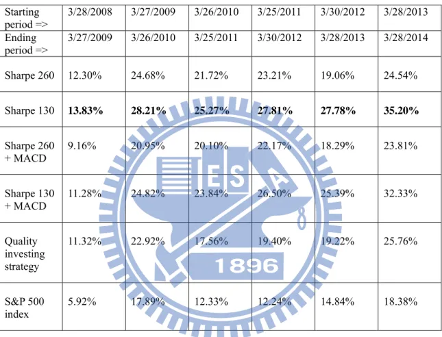
Table 4 Results of methodology number 2.Cumulative return rates of proposed technical strategies and benchmarks fundamental strategy and S&P 500 index

Starting period => 3/28/2008 3/27/2009 3/26/2010 3/25/2011 3/30/2012 3/28/2013 Ending period => 3/27/2009 3/26/2010 3/25/2011 3/30/2012 3/28/2013 3/28/2014 Sharpe 260 12.30% 24.68% 21.72% 23.21% 19.06% 24.54% Sharpe 130 13.83% 28.21% 25.27% 27.81% 27.78% 35.20% Sharpe 260 + MACD 9.16% 20.95% 20.10% 22.17% 18.29% 23.81% Sharpe 130 + MACD 11.28% 24.82% 23.84% 26.50% 25.39% 32.33% Quality investing strategy 11.32% 22.92% 17.56% 19.40% 19.22% 25.76% S&P 500 index 5.92% 17.89% 12.33% 12.24% 14.84% 18.38%

The summary from research design methodology number 2 confirmed unambiguously the results observed by methodology number 1. According to

methodology number 2, Sharpe ratio has been proved significantly as it has outperformed all other methods in all six observations.

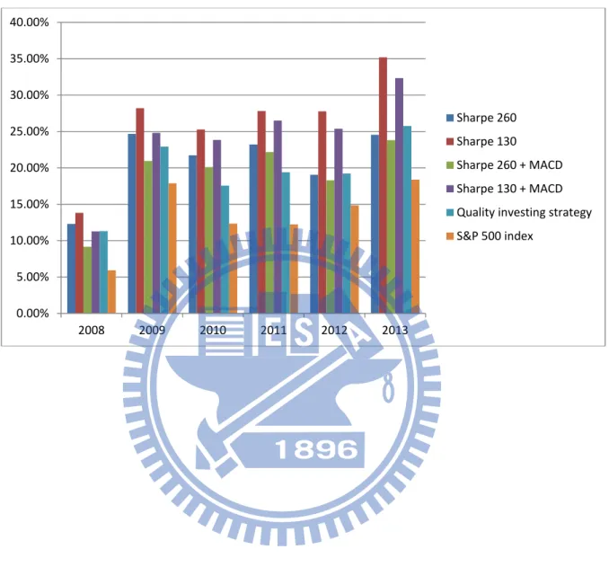
Figure 2 Compound return of technical strategies - methodology number 2 0.00% 5.00% 10.00% 15.00% 20.00% 25.00% 30.00% 35.00% 40.00% 2008 2009 2010 2011 2012 2013 Sharpe 260 Sharpe 130 Sharpe 260 + MACD Sharpe 130 + MACD Quality investing strategy S&P 500 index

Section 5: Conclusion

The goal of this study was mostly two fold. The first goal was to test whether 2 simple criteria of technical analysis applied on top of fundamental can improve the return rate of portfolios. This study indicates that investors can benefit from incorporating simple technical indicators to enhance their profitability. The best results are achieved by indicator Sharpe 130. The reason why Sharpe 130 brings better results when compared with Sharpe 260 lies probably in fact. That by empirical observation on the market it can be noticed that most stock prices, in essence, meander around dominant long trends. If that company is oscillating around the main trend for a roughly three month period before it makes a full circle. From this, it can be concluded that Sharpe 130 is better at

accommodating this natural behavioral characteristic of stock prices than Sharpe 260 which, is calculated from period which is simply too long and does not fully reflect those characteristics.

The research also shows that MACD utilized under the conditions set in this thesis did not show any practical usefulness. It can be pinned down to the fact that in a long term investing time frame it simply does not match the short term utility of MACD indicators.

The second goal of the study is to propose a simple and profitable implication of technical analysis for average retail investors. The Sharpe 130 is fulfilling this criteria, because in its nature it is very easy to calculate and it brings remarkable improvement of

having investment strategies utilizing both fundamental and technical analysis, and this research shows that the best results are achieved when Sharpe 130 is taken into

Study Limitations and Recommendation for Future Work

It is important to note the methodological limitations of the studies involved in this thesis. An important limitation in this research is the reliance on pre-selected data sample. This research has been performed as a follow up of preceding fundamental analysis, meaning it has been applied to those S&P 500 companies which have, based on fundamental criteria, already survived the short listing process. Although the results presented here have demonstrated the increase in profitability after applying the Sharpe 130 technical strategy, the conclusion from this study is limited as there may be questions as whether Sharpe 130 technical strategy would obtain the same results applied for instance, on entire S&P 500 (or any other) set of companies. Future research would benefit from studying presented technical strategies on a standalone basis. Such a design could allow stronger conclusions about the relationship, as presented in this thesis, between fundamental and technical analysis.

Another important limitation is based on the fact that companies listed in S&P 500 are principally large-cap companies that have, in general, lower volatility then small-cap companies. Since volatility is one of the key components for calculating Sharpe Ratio, future research would also benefit from testing the performance of presented technical strategies on companies of all capitalization ranges, in order to test the robustness of this strategy throughout the spectrum of companies with different statistical properties.

References

Brock, W., Lakonishok, J., & LeBaron, B. (1992). Simple technical trading rules and the stochastic properties of stock returns. The Journal of Finance, 47(5), 1731-1764)

Buranovsky, M. (2014). Quality Based Investing Strategy: Investing Based on

Fundamentals. NCTU Master Thesis.

Fama, E. F., & Blume, M. E. (1966). Filter rules and stock-market trading. Journal of

Business, 226-241.

Fama, E. F. (1991). Efficient capital markets: II. The journal of finance, 46(5), 1575-1617. Fama, E. F. (1998). Market efficiency, long-term returns, and behavioral finance. Journal

of financial economics, 49(3), 283-306.

Fong, W. M., & Yong, L. H. (2005). Chasing trends: recursive moving average trading rules and internet stocks. Journal of Empirical Finance, 12(1), 43-76.

Jensen, M. C., & Benington, G. A. (1970). Random walks and technical theories: Some additional evidence. The Journal of Finance, 25(2), 469-482

Keating, C., & Shadwick, W. F. (2002). An introduction to omega. AIMA Newsletter.

Malkiel, B. G., & Fama, E. F. (1970). Efficient capital markets: A review of theory and empirical work*. The journal of Finance, 25(2), 383-41.

Rom, B. M., & Ferguson, K. W. (1994). “Portfolio Theory is Alive and well” A Response. The Journal of Investing, 3(3), 24-44.

Schwager, J. D. (2012). Stock market wizards: interviews with America's top stock

traders (Vol. 94). John Wiley & Sons.

Sharpe, W. F. (1966). Mutual fund performance. Journal of business, 119-138.

Sharpe, W. F. (1994). The Sharpe Ratio. The Journal of Portfolio Management, 49-58.

Sharpe, W. F. (1998). Morningstar's risk-adjusted ratings. Financial Analysts Journal, 21-33.

Sullivan, R., Timmermann, A., & White, H. (1999). Data s­ nooping, technical trading rule performance, and the bootstrap. The journal of Finance, 54(5), 1647-1691.

Taylor, M. P., & Allen, H. (1992). The use of technical analysis in the foreign exchange market. Journal of international Money and Finance, 11(3), 304-314.

Appendix 1

Table 5 Stocks according tic symbols included in portfolios constructed on the basis of fundamental methodology "Quality based investing strategy" (Buranovsky, 2014)

Portfolio Companies Total

sum 2008 HON, ED, GE, IBM, ETR, MMM, RTN, TXN, UNP, WYE, GR, SHW,

BAX, GPC, DIS, GWW, AAPL, HAS, RDC, NOC, NWL, TMK, PX, SCHW, BEN, BMC, CPWR, AW, COL, BIIB, BXP, TEX, ESV, AVB, SUNE

35

2009 HON, IBM, ETR, XEL, RTN, GR, HNZ, BAX, GWW, AAPL, PLL, ORCL, PX, PPL, BIG, SWY, CPWR, COL, MON, BIIB, LLL, FOXA, CHRW, FLS, DO

25

2010 ABT, BMY, CL, IBM, XEL, RTN, BAX, BDX, CSC, GPS, SYY, CA, MIL., AMGN, AGN, AZO, BIG, SYK, MON, BIIB, CRM, PCLN, URBN

23

2011 BMY, HSY, IBM, MCD, GPS, SYY, AMGN, SIAL, AZO, BIG, LEG, SYK, FISV, VAR, HCBK, TDC, AMT, VTR, PCLN, ROST, URBN, CERN

22

2012 BMY, HSY, IBM, MCD, FDX, MAT, NOC, JWN, MMC, HD, SIAL, CBS, M, AZO, KSS, BBBY, SBUX, FDO, NVDA, PRU, AN, STZ, GNW, WFM, CME, CTSH, RL, NYX, LIFE, ORLY, TWC, DV, PCLN, FFIV, PRGO, BWA

36

2013 BA, CAT, XOM, IBM, ROK, UNP, SHW, GPC, IFF, DIS, WFC, VFC, SNA, NOC, PF, ITW, MMC, HD, ORCL, COST, CBS, M, EMC, AZO, ADBE, PNW, HOG, HOT, RHI, INTU, CTAS, FDO, SPG, AN, VLO, STZ, GNW, WFM, KIM, FIS, DTV, AVB, RL, ICE, HCP, PM, IVZ, ORLY, TWC, ARG, PCLN, BLK, ACN, PETM, DG

Appendix 2

Figure 3 List of the companies according investing strategies based on technical analysis

Note: that in Portfolio 2008 is change in inner structure between Sharpe 260 and Sharpe 260 + MACD as well as between Sharpe 130 and Sharpe 130 + MACD, because

company under tic symbol "SUNE" did not generate any MACD buy signal within designated period, therefore I include first following company according Sharp ratio ranking

Appendix 3

Figure 4 Sample of MACD computations

Autobiography

Name: Daniel Ziak Email: [email protected]

Nationality: Slovakia (斯洛伐克)

EDUCATION

Sep. 2012 – Jun.

2014 National Chiao Tung University (NCTU), Taiwan (國立交通大

學) – Global MBA (企業管理碩士) – AACSB accredited

international program in business administration focusing on entrepreneurship, strategic market management and new market development

Sep. 2003 – Jun. 2009 University of Economics in Bratislava, Slovakia – Major: Finance, Banking, Investment

Nov. 2011 – Jul. 2011 Trinity College London, United Kingdom – English Language

EMPLOYMENT HISTORY

Jun. 2012 – Jul.

2012 T-Systems International GmbH  Position: Process Expert

 Responsibilities: Process controlling, responsibility & authority in change and implementing of processes

Mar. 2011 - May.

2012 Office of Self-governing region Presov, Slovakia – Department of Regional Development

 Position: Control Manager

 Responsibilities: Performing of the financial control of payments from EU funds

Nov. 2009 – Mar. 2011

Social Implementing Agency (Ministry of Labour, Family and Social Affairs of Slovak Republic) Kosice, Slovakia

Position: Financial Manager

 Responsibilities: Managing investment projects funding by EU

FURTHER INFORMATION

Language skills Slovak – native, Czech – fluent, Polish - fluent, English – fluent

(TOEFL iBT -99/120), German – fluent (VHS Munich Level B1),

Computer skills MS Office (Word, Excel, PowerPoint, Outlook), basics of, Statistical