國立交通大學
交通運輸研究所
碩士論文
新興國家高速鐵路路線:以烏克蘭為例
Planning a High Speed Rail Route in an Emerging Country: A
Case Study of Ukraine
指導教授:
馮正民老師
林楨家老師
研 究 生:
韓安東
新興國家高速鐵路路線:以烏克蘭為例
Planning a High Speed Rail Route in an Emerging Country: A Case Study of
Ukraine
指導教授: 馮正民老師
林楨家老師
Advisors: Professor Cheng-Min Feng Professor Jen-Jia Lin
研 究 生: 韓安東 Student: Anton Hagen
國 立 交 通 大 學
交 通 運 輸 研 究 所
碩 士 論 文
A thesis
Submitted to Institute of Traffic and Transportation Management
College of Management
National Chiao Tung University
in partial Fulfillment of the Requirements
for the Degree of
Master
in
Traffic and Transportation
June 2013
Taipei, Taiwan, Republic of China
中華民國一 O 二年六月
i
Chinese Abstract
烏克蘭為歐洲大陸中幅員廣大的國家之一,具有主要城市彼此座落甚遠的特性。目前其 陳舊之鐵路網絡,僅能提供耗時的日間服務或隔夜班車,從首都基輔至西部、東部和南部 的市中心需要八至十二小時。這不僅限制了國境內交通機動性,且成為區域發展的障礙。 雖然烏克蘭鐵路在 2012 年歐洲足球錦標賽前進行改善,但其引進的 IC +列車並未解決烏 克蘭鐵路所面臨的挑戰。由於引進高速鐵路(high speed rail, HSR)是已開發國家為運輸改善 政策主流,故本研究著重建立針對烏克蘭高速鐵路的路線規劃方法。其研究目的為以下兩 點:1.引發烏克蘭國內對高速鐵路規劃的科學性方法的討論,並進一步提出適於烏克蘭高 速鐵路計劃的方法;2.本研究將規劃連接基輔與烏克蘭最東部的商業中心-頓涅茨克之高 速鐵路路線。 本研究的規劃方法分為兩個階段:方案產生(alternative generation)和方案評估(alternative evaluation)。第一階段為列出鐵路路線的替選方案,此階段目的為列舉可能的路線及定義 排除不可行方案的準則。本研究透過電腦模擬列出所有可能的路線,並採用階層分析法 (analytic hierarchy process , AHP)及理想解類似度順序偏好法(technique for order of preference by similarity to ideal solution , TOPSIS),以選擇替代路線做進一步的評估。第 二階段使用運輸需求分析(transportation demand analysis , TDA)和地 理資訊系統(geographic information system , GIS),針對每條路線的特徵進行分析,最終確定最適路 線。 本研究的主要貢獻為以下兩點:1.提供一高速鐵路路線規劃之方法;2.並依據建議參考 之評選準則提出最佳之高速鐵路路線規劃。所建議之最佳路線為連結基輔、切爾卡瑟、克 里沃羅格、聶伯城及頓涅茨克等城市。本研究所提出之方法與成果可作為後續研究之參考, 後續研究者可依據本研究之基礎提出進一步之觀點及成果,或是發展相關議題,如本研究 建議路線之可行財務方案。 關鍵詞:高速鐵路、路線規劃、多準則決策。
ii
English Abstract
Ukraine is one of the largest countries of Europe and its major cities are situated far away from each other. The current railway network is obsolete and provides either overnight or time-consuming daytime service, so it takes 8-12 hours to get from the capital city of Kyiv to the regional centers in the West, East and South. This limits mobility inside the country and creates obstacles for regional development. Although Ukrainian railroads were improved before the UEFA Euro 2012 Championship, introduction of IC+ trains did not solve challenges of Ukrainian railroad. As high speed rail (HSR) introduction is a mainstream in transportation improvement policies in developed countries, this research makes an attempt on developing a route planning approach for Ukrainian HSR. This study aims at two objectives: to start a scientific discussion of HSR in Ukraine, and to propose a method, that can be used in further HSR planning in Ukraine. The HSR line offered will connect Kyiv with Donetsk, the most eastern business center of Ukraine.
This study develops the planning approach in two main phases: alternative generation and alternative evaluation. The first phase generates route alternatives. The most important components of this phase are identifying possible routes and defining rules to cut off infeasible alternatives. The possible routes are identified via a computer simulation that generates the full list of the routes available. Using analytic hierarchy process (AHP) and technique for order of preference by similarity to ideal solution (TOPSIS), the alternative routes are selected for further evaluations. The second phase uses transportation demand analysis (TDA) and geographic information system (GIS) to analyze the characteristics of each route and finally determine the optimal route.
This study results in two contributions: it introduces a method of HSR route planning and recommends the optimal HSR route considering the chosen criteria. The route connects Kyiv, Cherkasy, Kirovohrad, Kryvy Rih, Dniprodzerzhyns’k, Dnipropetrovs’k, Zaporizhzhya and Donetsk. The proposed methods and results of this study can be used for the further studies in this field. Future researchers can either improve the ideas and results of this study or develop neighboring issues such as possible financing scenarios according to the results of this study.
iii
Acknowledgement
I would like to express my deep gratitude to my advisors Professor Cheng-Min Feng and Professor Jen-Jia Lin for their patient guidance, enthusiastic encouragement and useful critiques of this study. I would also like to thank the experts who spent their valuable time on filling in the AHP surveys.
I would like to extend my thanks to my classmates for introducing me the life in Taiwan helping me to overcome the language barrier.
Finally, I wish to thank my parents and my sister for their support and encouragement throughout my study.
iv
Contents
Chinese Abstract ... i English Abstract ... ii Acknowledgement ... iii List of Tables ... viList of Figures ... viii
I. Introduction ... 1
1.1 Motivations and background ... 1
1.2 Research objectives ... 4
1.3 Research scopes... 5
1.3.1 Key terms ... 5
1.3.2 Spatial and temporal scopes ... 5
1.4 Research process ... 6
II. Literature Review ... 9
2.1 HSR studies review ... 9
2.2 Methodology review ...12
III. Route Planning Methods ... 16
3.1 Computer simulation ...16
3.2 TOPSIS ...23
3.3 AHP ...25
3.4 Transportation demand analysis ...26
3.5 Construction complexity assessment...27
3.6 External effects evaluation ...27
IV. Case Study ... 27
4.1 Alternative generation ...27
4.1.1 Route generation ...27
4.1.2 Route ranking ...31
4.1.3 Route grouping ...34
4.2 Alternative evaluation ...37
4.2.1 Transportation demand analysis ...37
4.2.2 Construction complexity evaluation ...46
v
4.2.4 Decision about the optimal route ...52
V. Conclusions and Recommendations ... 55
References ... 57
Appendix 1 AHP questionnaire #1 ... 59
Appendix 2 AHP questionnaire #2 ... 63
vi
List of Tables
Table 1 Top-10 cities, by population (1 Jan. 2012) ... 2
Table 2 Price comparison: IC+, Overnight premium and Overnight ordinary ... 4
Table 3 Route search example ... 21
Table 4 Decision matrix ... 23
Table 5 Pair wise comparison table ... 25
Table 6 Comparison matrix ... 25
Table 7 Weights of criteria ... 32
Table 8 Route alternatives ... 33
Table 9 List of the alternatives, after grouping ... 35
Table 10 Final list of the routes ... 35
Table 11 Regression statistics ... 40
Table 12 Coefficiens ... 40
Table 13 Second regression statistics ... 41
Table 14 Second regression statistics (2) ... 41
Table 15 Coefficients of the second regression ... 42
Table 16 Residuals' statistics ... 43
Table 17 Observed frequencies vs. expected frequencies ... 44
Table 18 Travel demand for each route ... 46
Table 19 Lengths of sensitive area crossings at each section ... 48
Table 20 Lengths of sensitive area crossings at each route ... 48
Table 21 Built-up area crossing and water body crossing indexes ... 49
Table 22 Bad slope index ... 50
Table 23 Construction complexity summary ... 50
Table 24 External effects summary ... 51
Table 25 Criteria values for the alternatives ... 52
Table 26 Weights of criteria ... 53
Table 27 Integrated weights ... 54
Table 28 Route rankings ... 54
Table 29 Route 1 demand ... 68
vii
Table 31 Route 3 demand ... 69 Table 32 Route 4 demand ... 69 Table 33 Route 5 demand ... 70
viii
List of Figures
Figure 1 Approximate socio-economic pattern of Ukraine. ... 1
Figure 2 Area of possible routes from Kyiv to Donetsk. ... 6
Figure 3 Research process ... 8
Figure 4 Average external costs per transportation mode ... 9
Figure 5 Air services between Paris and Brussels ... 10
Figure 6 Number of passengers for London-Paris link ... 11
Figure 7 Planning process ... 17
Figure 8 Search function step example. ... 18
Figure 9 Route generation algorithm ... 20
Figure 10 Cities, located at the map in the iMap Creator ... 29
Figure 11 Map, opened in the Route Planner ... 29
Figure 12 Route list window ... 30
Figure 13 Visual representation of all possible routes ... 30
Figure 14 Ranked list of routes, top 5 selected ... 33
Figure 15 Visual representation of top-5 routes, without grouping ... 34
Figure 16 Final top-5 routes for analysis ... 36
Figure 17 Residuals of the second regression ... 42
Figure 18 Route 5 traced over the topographic map ... 47
Figure 19 Loaded DEM data in ArcGIS ... 49
Figure 20 The optimal route ... 54
1
I. Introduction
1.1 Motivations and background
Ukraine is an emerging country of Eastern Europe, former USSR. According to CIA World Factbook, it is the second largest country of Europe (and the first one, if Overseas France is not considered); its square is 603.6 thousand km2, east-west distance – 1300 km, and north-south distance – 900 km. The population of Ukraine is around 46 million of people. As this research will often consider socio-economic geography of Ukraine, it is important to provide here more information about the country, as shown in Figure 1.
Background map source: http://worldmap.org.ua/ Figure 1 Approximate socio-economic pattern of Ukraine.
Socio-economic pattern of Ukraine varies a lot from East to West and from North to South. It is caused by heavy industries that are concentrated in the south-east of Ukraine. Those industries where formed during 1930-s and stimulated population increase in the existing cities and created new ones. So, along with high industrialization, east of Ukraine can be characterized as highly-urbanized. There are also smaller places with industry in the center and west of Ukraine (vehicle
2
production, chemical industries), that explains high urbanization level in Lviv region, for example, but most of chemical industries are now closed. The north-east and center are mainly agricultural areas and the north-west is covered with forests, so the population density is low there.
Table 1 Top-10 cities, by population (1 Jan. 2012) Cities Population Kyiv (capital) 2 814 258 Kharkiv 1 441 362 Odesa 1 008 162 Dnipropetrovs'k 999 577 Donets'k 955 041 Zaporizhzhya 772 627 Lviv 729 842 Kryvy Rig 660 203 Mykolaiv 497 032 Mariupol 464 457
Although major cities are mainly situated in the east and center of Ukraine, there are still quite large and economically important cities in the west. This leads to the problem of intercity transportation in Ukraine: large cities are situated far away from each other. For instance, Lviv and Donetsk (western and eastern regional centers respectively) are 1.200 km away from each other.
At the moment, the main way of intercity transportation in Ukraine is an obsolete railway network, originally built for freight transportation. This causes the following weaknesses of transportation system:
1. Average speed is quite low, the fastest daytime train has average speed of 116 km/h, the fastest overnight trains – around 60-65 km/h. This leads to very long travel times (for case of Lviv-Donetsk travel, it will be 18-20 hours).
2. Railroad routes are not direct and/or deviate from large cities.
Because of low speeds and long distances, overnight travelling is widespread in Ukraine. Still, though this model is relatively comfortable for 8-10 hours trip, it is almost unacceptable for 20 hours trip. These weaknesses break social and economic relations inside the country and strongly limit business activities.
In order to improve railway services, the government developed a program of InterCity+ (IC+) traffic on existing tracks, but there was no public discussion; therefore, no information if the government considered HSR alternative for Ukraine is available.
3
During preparation to Euro-2012 championship, the major directions of Ukrainian railroad system were improved to allow continuous maximum speed of 160 km/h and new rolling stock from Hyundai Rotem was purchased (10 trains). At the moment these trains are commuting on routes Kyiv-Kharkiv (3 per day), Lviv-Kyiv, and Kyiv-Donetsk (2 per day).
Nevertheless, these changes haven’t improved the situation much: only services of Kyiv-Kharkiv are relatively successful and, for other two routes, the following shortcomings exist.
1. Number of stops
Existence of intermediate stops is often very important: it helps to generate demand for transportation. Roughly, if you have route A to B with a stop C, there will be two types of traffic of each section (AC: A -> C, A -> B, CB: C -> B; A -> B). Currently Lviv route doesn’t have intermediate stops because there are no large cities along the used track.
2. Travel times
Travel time is one of the measures that drastically influences travel demand. If the train doesn’t show significant difference from conventional rail, it will not be popular. For example, there is an alternative way from Kyiv to Lviv that has 3 more large cities, but it will increase travel time from 5 hours to 6.5 hours. In the same time, the main trouble of Donetsk route is also travel time: it takes 6.5 hours to get to Donetsk.
3. Convenience
IC+ trains travel during daytime and it is not convenient for numerous people. For example, when business trip is necessary, employer will want his employee to return from a trip as soon as possible. If business requires a 2-day 9 a.m. - 18 p.m. presence in the other city, it means that the entire trip will take 4 days and 2 more nights in hotel. On the other hand, overnight train is much more convenient in term of time usage: the trip can start right in the end of working day and next morning that person is doing his job in another city.
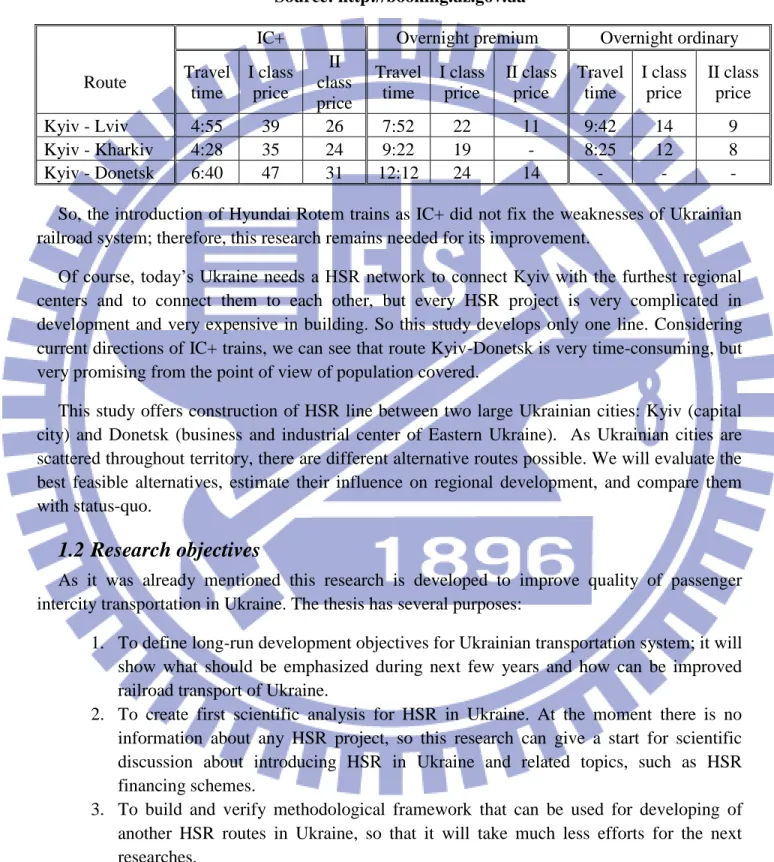
4. Price
Ticket price for IC+ train is almost 90% higher than in premium-class overnight trains as shown in Tab. 2. In pair with relative inconvenience of IC+, this price scares away the passengers.
4
Table 2 Price comparison: IC+, Overnight premium and Overnight ordinary Source: http://booking.uz.gov.ua
IC+ Overnight premium Overnight ordinary
Route Travel time I class price II class price Travel time I class price II class price Travel time I class price II class price Kyiv - Lviv 4:55 39 26 7:52 22 11 9:42 14 9 Kyiv - Kharkiv 4:28 35 24 9:22 19 - 8:25 12 8 Kyiv - Donetsk 6:40 47 31 12:12 24 14 - - -
So, the introduction of Hyundai Rotem trains as IC+ did not fix the weaknesses of Ukrainian railroad system; therefore, this research remains needed for its improvement.
Of course, today’s Ukraine needs a HSR network to connect Kyiv with the furthest regional centers and to connect them to each other, but every HSR project is very complicated in development and very expensive in building. So this study develops only one line. Considering current directions of IC+ trains, we can see that route Kyiv-Donetsk is very time-consuming, but very promising from the point of view of population covered.
This study offers construction of HSR line between two large Ukrainian cities: Kyiv (capital city) and Donetsk (business and industrial center of Eastern Ukraine). As Ukrainian cities are scattered throughout territory, there are different alternative routes possible. We will evaluate the best feasible alternatives, estimate their influence on regional development, and compare them with status-quo.
1.2 Research objectives
As it was already mentioned this research is developed to improve quality of passenger intercity transportation in Ukraine. The thesis has several purposes:
1. To define long-run development objectives for Ukrainian transportation system; it will show what should be emphasized during next few years and how can be improved railroad transport of Ukraine.
2. To create first scientific analysis for HSR in Ukraine. At the moment there is no information about any HSR project, so this research can give a start for scientific discussion about introducing HSR in Ukraine and related topics, such as HSR financing schemes.
3. To build and verify methodological framework that can be used for developing of another HSR routes in Ukraine, so that it will take much less efforts for the next researches.
5
1.3 Research scopes
1.3.1 Key terms
The key concept used in this thesis is High Speed Railroad, shortly HSR. There are different understandings of HSR, first of all because of different maximum speeds. In the study HSR is a railway system (infrastructure and rolling stock) that allows high speed movement up to 300 km/h and approximate average speed of 200 km/h.
On the contrary to HSR, conventional railroad is a basic railroad system, created during XIX-XX centuries with a priority in freight transportation. Consequently this railway network is bound to freight demand-generating nodes and is not fully efficient for passenger transport. Speed on conventional railroads is limited to 140 km/h, on major lines – to 160 km/h.
There are also two terms in this research, that sound very similarly - HSR route and HSR line, but they should not be mixed. HSR route is a route available for usage by high speed train at lower speed, while HSR line is an exclusive line for high speed trains. This division is necessary for the case of mixed HSR route, when it can include both HSR lines and conventional railroad lines.
1.3.2 Spatial and temporal scopes
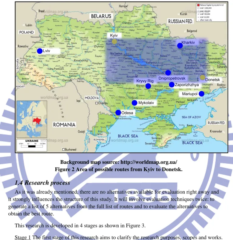
This thesis aims at developing an approach to determine the optimal HSR line between Kyiv and Donetsk, which is the most eastern large business city. There are numerous possible routes, but the most probable are routes via Kharkiv (the largest city in the eastern Ukraine) or via Dnipropetrovsk and some smaller cities. Theoretically the most possible routes will lie in the highlighted area of Figure 2.
In terms of time, this project cannot be regarded as a short-run. In fact, HSR project is a financial and engineering challenge that means that every stage of its implementation will be time-consuming. For example, it took 7 years for Taiwan to build a 350-km HSR, so even if conditions in Ukraine are much easier, it will probably take about 15 years to build a 650-km line between Kyiv and Donetsk.
Still, the time of project implementation strongly depends on the type of financing that will be chosen for the project and from the route selected. For example, if the line will be built on the left side of the Dnieper River, it will require significantly less special structures like bridges and tunnels, because of flat terrain. It will reduce price and improve the speed of building. One more important example: in case line is compatible with conventional railroad (like in France or Germany), it will be possible to introduce HSR partially, temporarily including upgraded conventional rail into the system.
6
Background map source: http://worldmap.org.ua/ Figure 2 Area of possible routes from Kyiv to Donetsk.
1.4 Research process
As it was already mentioned, there are no alternatives available for evaluation right away and it strongly influences the structure of this study. It will involve evaluation techniques twice: to generate a list of 5 alternatives from the full list of routes and to evaluate the alternatives to obtain the best route.
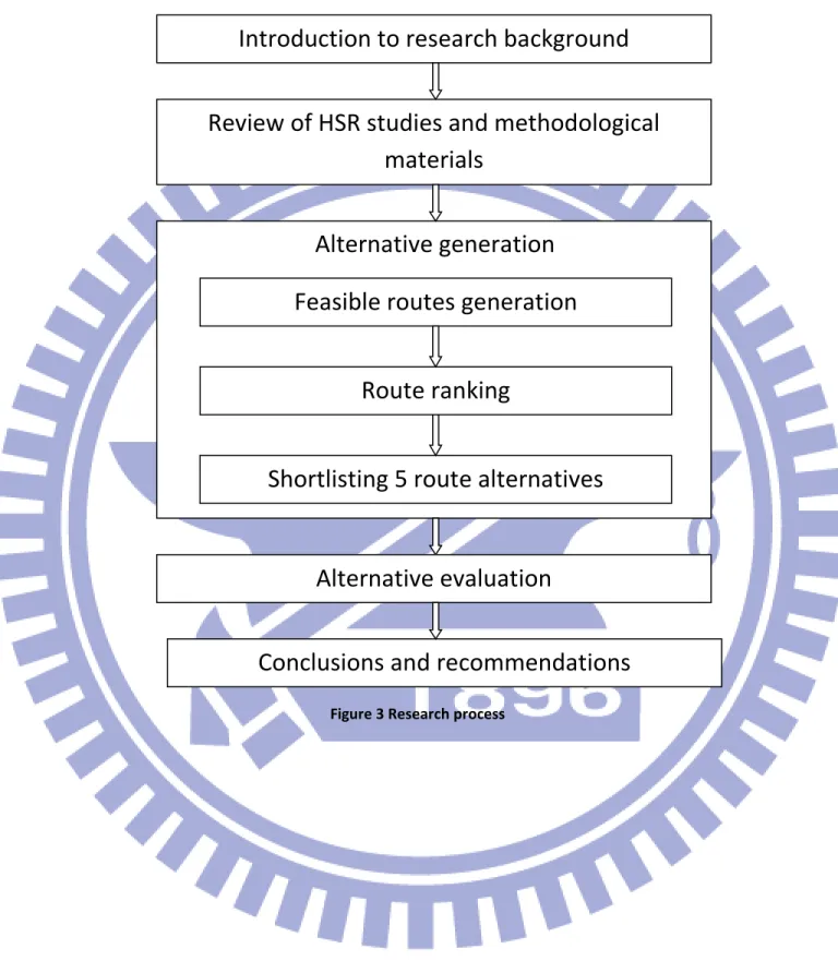
This research is developed in 4 stages as shown in Figure 3.
Stage 1 The first stage of this research aims to clarify the research purposes, scopes and works. Therefore, the data about Ukrainian geography, socio-economic pattern and current state of intercity transport is generalized on the first stage in order to create a general idea about the direction of the project.
Stage 2 This stage is devoted to literature review in order to examine previous studies in the field of project. There are three directions of literature review:
7
literatures that study HSR projects in the other countries;
methods in the fields of transportation routing, demand estimation and project evaluation.
Stage 3 In this stage, the route planning method proposed in this study is described. Stage 4 Case study
Stage 4.1 Alternative generation At first, a simplified routing algorithm is used that will produce all possible routes between the origin and the destination. Then they will be ranked by three criteria: route population, route length, and route curvature:
1. Route population (max). This criterion is an incentive for a HSR route to pass though maximum possible number of cities, because every new city on the route can generate new demand.
2. Route length (min). This criterion is an incentive for route length minimization because long route increases travel time and building cost.
3. Route curvature (min). This criterion is an incentive to make a HSR route as straight as possible, without covering the cities that are located far from the direct route between the origin and the destination.
As we are facing three-criteria optimization and those criteria have different preference direction, TOPSIS is used to balance these criteria and assign overall criteria satisfaction score to each alternative route.
Stage 4.2 Alternative evaluation Values for alternatives are evaluated.
Stage 4.2.1 Approximate transportation demand estimation for each feasible route using travel demand analysis.
Stage 4.2.2 Measurement of construction complexity criteria values. Stage 4.2.3 Measurement of external effects criteria values.
Stage 4.2.4 Selection of the most optimal route based on the criteria of route travel demand, construction complexity, and external effects.
8
Introduction to research background
Review of HSR studies and methodological
materials
Alternative generation
Feasible routes generation
Route ranking
Shortlisting 5 route alternatives
Conclusions and recommendations
Alternative evaluation
9
II. Literature Review
2.1 HSR studies review
Literature review of this research could include the following three topics:
review of the literature, that directly concerns the topic of HSR development in Ukraine;
review of studies, devoted to HSR development in different countries;
general review of decision-making techniques about route planning.
Unfortunately, the first topic cannot be represented in this review: after investigations performed, no research papers were found on the topic. So, we assume that this research is the first known study of HSR in Ukraine and skip the first section of review.
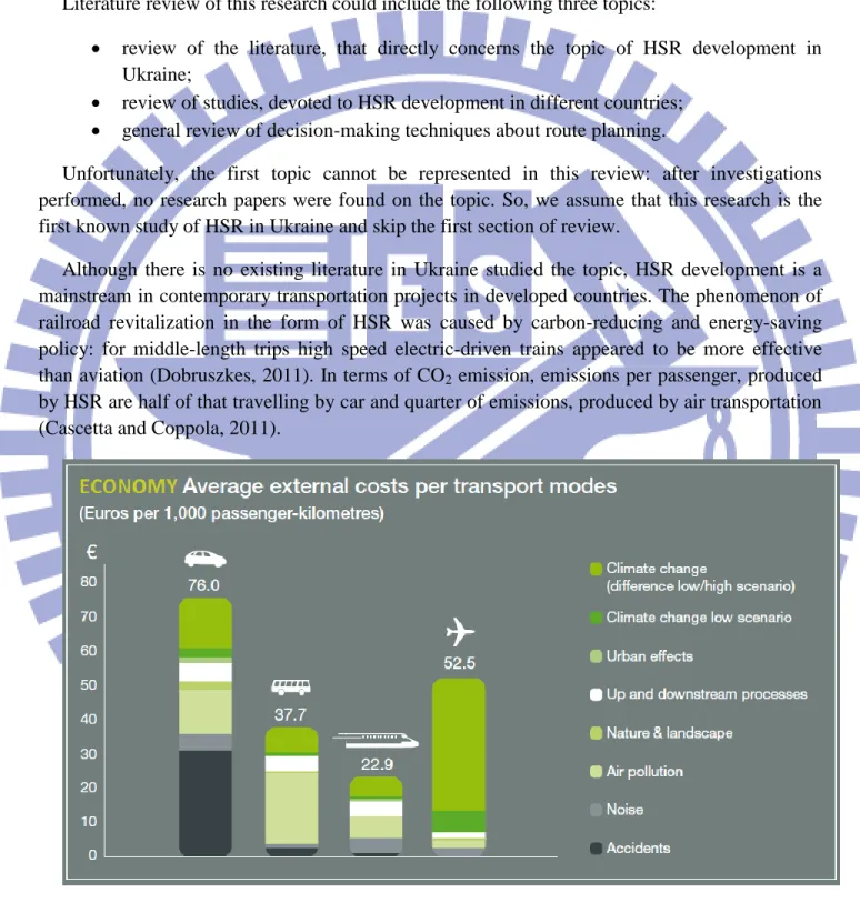
Although there is no existing literature in Ukraine studied the topic, HSR development is a mainstream in contemporary transportation projects in developed countries. The phenomenon of railroad revitalization in the form of HSR was caused by carbon-reducing and energy-saving policy: for middle-length trips high speed electric-driven trains appeared to be more effective than aviation (Dobruszkes, 2011). In terms of CO2 emission, emissions per passenger, produced
by HSR are half of that travelling by car and quarter of emissions, produced by air transportation (Cascetta and Coppola, 2011).
Source: UIC (2010)
10
As it can be seen on the Figure 4, there are strong incentives to encourage modal shift from aviation and cars to HSR lines, as it influences environment less that other modes.
There is also a significant difference in the land use. While standard double-track railway line requires 25 m wide line, a 6-lane motorway requires 75 meters (the area occupied is 3.2 ha/km and 9.3 ha/km respectively), but the capacity is almost the same. Moreover, there is a common practice to build HSR lines parallel to existing motorway that helps to reduce land use significantly (UIC, 2010).
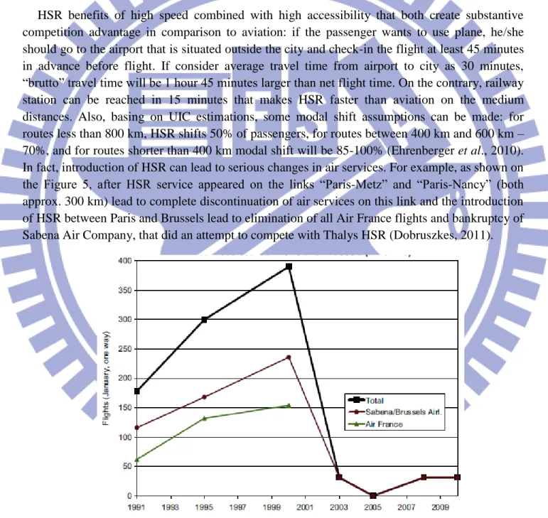
HSR benefits of high speed combined with high accessibility that both create substantive competition advantage in comparison to aviation: if the passenger wants to use plane, he/she should go to the airport that is situated outside the city and check-in the flight at least 45 minutes in advance before flight. If consider average travel time from airport to city as 30 minutes, “brutto” travel time will be 1 hour 45 minutes larger than net flight time. On the contrary, railway station can be reached in 15 minutes that makes HSR faster than aviation on the medium distances. Also, basing on UIC estimations, some modal shift assumptions can be made: for routes less than 800 km, HSR shifts 50% of passengers, for routes between 400 km and 600 km – 70%, and for routes shorter than 400 km modal shift will be 85-100% (Ehrenberger et al., 2010). In fact, introduction of HSR can lead to serious changes in air services. For example, as shown on the Figure 5, after HSR service appeared on the links “Paris-Metz” and “Paris-Nancy” (both approx. 300 km) lead to complete discontinuation of air services on this link and the introduction of HSR between Paris and Brussels lead to elimination of all Air France flights and bankruptcy of Sabena Air Company, that did an attempt to compete with Thalys HSR (Dobruszkes, 2011).
Source: Dobruszkes (2011)
11
Quite similar situation in on the link between London and Paris, but the aviation is not fully eliminated there, probably because of high fares for Eurostar trains and because London Heathrow airport often is not a final destination, but a hub (Dobruszkes, 2011). The competition between HSR and aviation on the link between London and Paris can be seen on the Figure 6.
Source: Behrens and Pels (2012)
Figure 6 Number of passengers for London-Paris link
HSR introduction causes not only modal shift on the OD pair, but also generates new demand, called induced demand. Changes in travel time and travel cost that can be referred as total trip cost change, they also can be a measure of accessibility (Yao and Morikawa, 2003). These changes in accessibility cause changes of socio-economic situation: changed travel times influence people’s choice of place and work. For example, people can move to other working places or move themselves to more living-convenient rural areas, becoming commuters (Cascetta and Coppola, 2011). This is the reason, why HSR lines in many countries are regarded as a way of regional development and decentralization (Ryder, 2012). The amount of induced traffic is usually very significant, that causes strong interest towards this phenomenon. For example, in France and Japan HSR produced additional traffic as high as 35%, and the study in the Canberra-Sydney obtained a value of 26% even without taking in consideration changes in land use that can happen in the long-term (Hensher, 1997).
12
2.2 Methodology review
There is a significant lack of studies in the field of route planning for railroads. Usually scientists evaluate given alternatives or make some specific studies about the project that already exists, but there are no commonly used methods, for the case, when the routes should be generated first. Nevertheless, some common methods of transportation will be used.
Regarding transportation routes evaluation, the most widespread are the studies devoted to demand estimation, assessment of external effects, such as air pollution, noise and vibration pollution, and influence on living areas.
The most generally-used model for demand estimation is transportation demand analysis (TDA). It consists of 4 stages: trip generation, trip distribution, modal shift, and traffic assignment.
According to Caulfield (2011), trip generation refers to the amount of trips generated by each origin and destination that are influenced by several socio-economic feature of the zone. It includes two components:
trip production (by the origin points), can be influenced by population, wages on the macro-level and by family size, social status, availability of car on the household level;
trip attraction (by destinations) is usually assumed to be influenced by the type of land use, economic activity, employment.
Trip distribution, as a second step of TDA, may be formed in different ways, but the most widely used is gravity approach to the distribution of trips. It assumes that trips from each origin towards each destination are distributed according to Newton’s gravity law as follows:
)
(
ij j i ijO
D
f
c
T
where Tij: travel amount on the link between cities i, j; α: proportionality factor;
Oi, Dj: trips, generated by origin i and destination j; f(cij): generalized function of travel cost between i and j.
Generally speaking f(cij) here is a resistance factor, so not only the cost can be used at this
place, but also travel time or distance.
Mode split is usually based on the utility of each alternative mode that consists of predicable value V and random value ε as follows:
m m m
v
u
where um: utility of mode m;
(1)
13
vm: predicable utility component of mode m; ε m: random utility component of mode m.
Predictable component is a function of the transportation mode characteristics, such as travel cost, travel time, additional costs, etc. Finally, using the utilities calculated, mode choice model is built as a multinomial logit model as follows:
i v v m i me
e
P
where Pm: probability of choosing mode m;
vm: predicable utility component of mode m.
The last step of the conventional model – traffic assignment – concerns link availability as a supply and number of O-D pairs and transportation modes as a demand. This step operates with a term of Level of Service (LOS) for each link of the network: the higher is the demand on each link, the worse are the traffic conditions and the larger is travel time. Mathematically:
S Q V
e
t
t
0 /where t: travel time at the link;
t0: travel time under free flow conditions; V: flow;
Qs: link capacity.
It should be taken into account that transferring an O-D pair from one link to another will simultaneously cause improvement of LOS on the former, and decline of LOS on the latter.
According to the purposes of analysis, this method can be used partially, depending on the detailing of analysis needed. Also, TDA can be used in several variations, depending on the data available. For example, Ehrenbreger et al. (2010) uses a TDA that joins stages 1 and 2 of the analysis for European HSR lines. This integrated model utilizes socio-economic data of two cities and passenger traffic on the link between them. The study develops a gravity model for European cities, where transportation demand can be estimated via GDP, tourism intensity, population size, and distance. In the final model tourism data is omitted, because it does not influence result.
where Fij: travel amount between cities i and j;
(3)
(4)
14
β0… β3: coefficients;
Pi, Pj: population of cities i and j;
Wi, Wj: GDP of cities i and j;
dij: distance between cities i and j;
vij: average speed on the link between i and j.
We should note that although the above study is devoted to the development of second-generation HSR, it offers methods, useful for this research.
Evaluation of HSR route requires not only travel demand data, but also information about engineering and environmental feasibility of the project. Depending on the accuracy level needed and available data, methods can vary from rather precise monetary evaluation to rough assessment, but generally they usually use Geographic Information Systems (GIS).
Both kinds of feasibility refer to the construction complexity, and, consequently, to construction cost. According to Uršej and Kontić (2007), it is influenced by such factors:
cost of special constructions, such as embankments, cuttings, bridges and tunnels;
cost of living-areas protection, such as noise and visual barriers;
cost of natural and cultural heritage protection: remediation of environment, creating crossings for animals;
additional cost, such as related to land purchase.
The key idea of route assessment in the study of Uršej and Kontić (2007) is thesis, that HSR should go underground, only in the cases, when surface solution is unavailable due to surface space, causes great negative environmental impacts, or is more expensive than subsurface alternatives. That’s why route planning starts form the suitability analysis of the surface where the alternative route should lie. Finally, alternative routes are ranked with respect to length of the route, number of tunnels and subsurface sections length.
GIS is also used in the study by Ehrenbreger et al. (2010) to evaluate technical complexity of the future line. This estimation is based on two ideas: there is a basic construction cost per kilometer and resistance multipliers that are calculated from resistance maps. At the resistance map, each raster pixel is assigned a resistance value depending on geographic conditions. Parameters that significantly influence construction cost are:
Slope of the terrain.
As railway lines are restricted to the maximum gradient (for HSR maximum is usually 35-40‰ on the exclusive tracks, (UIC, 2010)), the cases exceeding this limit have to be handled by building of embankments or tunnels, bridges. Bridges and tunnels are assumed to be 7 times more expensive than the basic cost value.
15
A higher population density leads to the higher construction costs, because such areas have a few free areas for HSR line. So, the population density over 100 persons per pixel causes linear growth of the resistance multiplier. If the population is less than 100 persons per pixel, it does not affect construction cost.
Water bodies.
Crossing of rivers is assign to have a resistance factor of 5.4, other water bodies cannot be crossed except the British channel. As it already has a tunnel, it has a small resistance factor of 1.5 (larger than 1 because of high fares).
More criteria for route evaluation can be found in California High Speed Rail Authority (2012) that develops HSR route in California, USA. One of the issues studied is a section of HSR between two cities and environmental impact of alternative routes. To evaluate the routes, two groups of criteria are introduced: physical and operational characteristics (such as travel time (minimization), intermodal connections (maximize), route length (minimize) etc.) and environmental impacts (air pollution, noise, vibrations, cultural and human hazards). Most of these criteria are already discussed, but there is one extra – intermodal connections, that helps to evaluate HSR line not only as a single transportation unit, but a part of transportation infrastructure of the region.
16
III. Route Planning Methods
This research uses different methods to obtain an optimal HSR route. These methods are: computer simulation, TOPSIS (technique for order of preference by similarity to ideal solution), AHP (analytic hierarchy process) and TDA (transportation demand analysis). The planning process is shown in the Figure 7 and explained as follows.
3.1 Computer simulation
Route evaluation studies usually concern an evaluation of existing route alternatives. In this study there are no given alternatives, so we have to generate them first. The literature studied does not give any method to generate alternative routes, so the route generation algorithm was developed specifically for this study.
To obtain route alternatives, we generate all possible routes between origin and destination; rank them according to the criteria and create a shortlist of 5 feasible rotes. Those feasible routes will be used further as alternatives for evaluation.
To generate full list of possible routes, this study uses recursive computer simulation to implement alternative generation algorithm that is based on the assumption that city population is a proxy to transportation demand it generates. Total sum of on-route city populations is used to roughly estimate total transportation demand of each route and rank the routes. Top routes will be considered as feasible and used for further analysis.
The classical TDA method is not used at this stage of the research, because its implementation for each route in the full list (that can theoretically contain hundreds and thousands of routes) will dramatically increase the computation complexity and time consumption of ranking, so that it will likely block the further progress of the study.
Simulation of the algorithm requires dataset with information about the cities. Each city record contains data about:
City name
17
Route ranking using
TOPSIS, with criteria:
1. Total population covered 2. Total route length
All possible routes
Recursive computer
simulation
Geospatial data &
Cities population
Top 5 routes are
alternatives for
future evaluation
TDA: 3 steps
1. Trip generation 2. Trip distribution 3. Mode choicefor each alternative
Socio-economic data about cities, contained in each
alternative
Travel demand for
each alternative
Alternative ranking
using TOPSIS with
criteria:
1. Travel demand 2. Construction complexity 3. External effects Engineering complexity dataExternal effects data
Optimal HSR route
Legend:
Input data Procedure Intermediate
data
18
In addition to this we need spatial information about the cities; this data is represented by distance matrix.
Let
C = {0, 1, …, i, … n}: set of cities;
co, cd ∈ C: are given origin and destination cities respectively;
cc ∈ C: current city – a city where the recursion is located at each moment;
D = [dij] ∀ i, j = 0..n, i ≠ j: a distance matrix, while dij is a distance between cities i and j;
Pi: population of city i, where i = 0..n;
T: population threshold (to exclude cities that too small to be considered in the simulation).
As the result of simulation we expect to have a set of routes R = {r0, r1… rm} where ri =(S, p, l, a) ∀ i = 0..m is a route; p - total population, l - length and a - curvature index of each route. City list S = (s0, s1, …, sn) is also a vector containing indexes of cities connected by the route i.
For running a recursion we need two additional variables associated with stack: recursive algorithm needs a “memory” to store current recursion depth and all previous steps. Let stack = (S, pos) be a vector of city list and position variable, where city list is the same vector as for route stack.S = (s0, s1, …, sn).
At the beginning we are situated at origin, so current city cc = co.
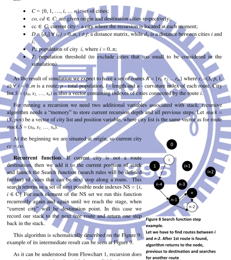
Recurrent function. If current city is not a route destination, then we add it to the current position of stack and launch the Search function (search rules will be defined further) of cities that can be next stop along a route. This search returns us a set of next possible node indexes NS = {i, i ∈ C} For each element of the NS set we run this function recurrently again and again until we reach the stage, when “current city” will be destination point. In this case we record our stack to the next free route and return one step back in the stack.
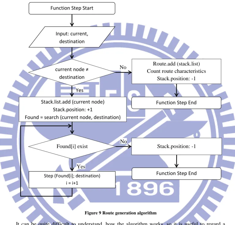
This algorithm is schematically described on the Figure 9; example of its intermediate result can be seen at Figure 9.
As it can be understood from Flowchart 1, recursion does not use given spatial and social data explicitly, it operates only with the next possible nodes, returned by the Search
0 1 i i+1 i+2 n n-4 n-1 n-2 n-3
Figure 8 Search function step example.
Let we have to find routes between i and n-2. After 1st route is found, algorithm returns to the node, previous to destination and searches for another route
19
function.
Search function. A very important module for route generation is the Search function. It considers information about the origin city (co ∈ C), current city (cc ∈ C), and destination city (cd∈ C) and tries if any of cities i ∈ C can be the next city on the route form cc to cd. The city is added to the output set of possible next cities NS, if all the following conditions are fulfilled:
1. Pi T : we take into account only cities with population over threshold level; 2. d[cc,cd]d[i,cd]: every next city should be closer to destination;
3. d[cc,cd]2d[cc,i]2d[i,cd]2: obtuse angle between current city, next city and destination is required;
4. d[stack.Spos1,i]2 d[stack.Spos1,cc]2 d[cc,i]2: obtuse angle between previous city, current city and next city is required;
5. d[co,cd]2d[co,i]2d[i,cd]2: obtuse angle between origin, next city and destination is required.
20
Figure 9 Route generation algorithm
It can be quite difficult to understand, how the algorithm works, so it is useful to regard a small example as illustrated in the Table
Having cities with indexes from 0 to 4, the algorithm finds all possible routes between given origin and destination subject to search rules. On the diagram you can see:
1. Circles with numbers as cities a. Black – ordinary city b. White – terminal city
c. Grey – current city at a given step Function Step Start
Input: current, destination
Stack.list.add (current node) Stack.position: +1
Found = search (current node, destination) current node ≠
destination Yes
Step (Found[i]; destination) i = i+1
No Route.add (stack.list) Count route characteristics
Stack.position: -1
Function Step End
Found[i] exist
Yes
No
Stack.position: -1
21
2. Arrows witch are interpreted as connections between the cities: a. Black dashed – possible forward-steps at current city b. Black solid – previous forward-steps
c. Grey dashed – backward-steps at current city d. Grey solid - previous backward-steps at current city
Table 3 Route search example
0
Let: Origin = 1 Destination = 4
Calling Function Step (1, 4) Algorithm started.
Stack.list = {1}; Stack.position = 0;
1
Function Step (1, 4)
First, algorithm searches all possible next points of the route. According to the search rules, cities 0 and 2 are not qualified to the next step (city 0 because of rule 2, city 2 because of rule 3) , so the set
NS = {3, 4}
Next origin is city 3 (NS0), call function
Step (3, 4) Stack.list = {1, 3}; Stack.position = 1; Routes = {}; current_city = 1; 2 Function Step (3, 4)
According to the search, only city 4 is qualified to the next step,
NS = {4}
Next origin is city 4, call function Step (4, 4) Stack.list = {1, 3, 4}; Stack.position = 2; Routes = {}; current_city = 3; 0 2 1 3 4 0 2 1 3 4 0 2 1 3 4
22
3
Function Step (4, 4)
As here origin = destination, we record current stack as a route and count one position back.
As this function was called in (2), we return to Function Step (3, 4)
Routes = {{1, 3, 4}}; Stack.position = 1; Stack.list = {1, 3}; current_city = 4; 4 Function Step (3, 4) NS = {4}
NS0 was already tested, so we step to
NS1. It is empty, so we go back one stack
position more.
As this function was called in (1), we return to Function Step (1, 4)
Stack.position = 0; Stack.list = {1}; current_city = 3; 5 Function Step (1, 4) Having NS = {3, 4}
NS0 was already tested, so we step to
NS1. Next origin is city 4, call function
Step (4, 4) Stack.list = {1, 4}; Routes = {{1, 3, 4}}; Stack.position = 1; current_city = 1; 6 Function Step (4, 4)
As here origin = destination, we record current stack as a route and count one position back.
As this function was called in (1), we return to Function Step (1, 4)
Routes = {{1, 3, 4}, {1, 4}}; Stack.position = 0; Stack.list = {1}; current_city = 4; 0 2 1 3 4 0 2 1 3 4 0 2 1 3 4 0 2 1 3 4
23
7
Function Step (1, 4) Having
NS = {3, 4}
NS0, NS1 were already tested, so we step
to NS2. It’s empty, we exit function Step
(1, 4). Algorithm terminated. Routes = {{1, 3, 4}, {1, 4}}; Stack.position = 0; Stack.list = {1}; current_city = 1;
So, for this example the algorithm produced 2 routes – route 1 including cities {1, 3, 4} and route 2 including cities {1, 4}.
This algorithm will return a list of all possible routes between origin and destination, where each route includes city list and route characteristics used as criteria for ranking.
3.2 TOPSIS
In this study multiple criteria evaluation method TOPSIS will be used twice:
Level 1 evaluation. After full list of routes is generated, it should be ranked according to the chosen criteria to select 5 feasible routes.
Level 2 evaluation. After transportation demand and other criteria for final evaluation are calculated, TOPSIS is used to select the best of 5 feasible routes.
TOPSIS is extensively used because it gives a mechanism to rank alternatives according to multiple criteria of different nature with different preference direction (either maximization, or minimization). Available alternatives with the values of criteria are written as a decision matrix, see Table 4
Table 4 Decision matrix
eij Preference direction j Wi A1 A2 … An i C1 {MIN|MAX} e11 e12 … e1n w1 C2 {MIN|MAX} e21 e22 … e3n w2 … … … … Cm {MIN|MAX} em1 em2 … emn wm
where A1…An are alternatives; C1…Cm are criteria;
eij are values of criteria Ci of the alternative Aj. 0
2 1
3
24
w1…wm are weights of the criteria.
As initially values of criteria are not comparable, so the matrix should be normalized:
min max min i i i ij ij e e e e r
where eij : values of criteria Ci of the alternative Aj.
eimax: maximum value among the alternatives Aj for the criteria Ci. eimin: minimum value among the alternatives Aj for the criteria Ci; rij: normalized values of criteria Ci of the alternative Aj. .
Then each rij is multiplied corresponding weight wi
ij i ij wr
v
where rij: normalized values of criteria Ci of the alternative Aj; vij: updated values of criteria Ci of the alternative Aj; wi: weight of the criteria Ci.
According to preference direction, minimum and maximum values of each criterion are taken to create vectors of positive ideal and negative ideal solutions. For example, if there are 3 criteria with preference direction of MAX, MIN, and MAX, the positive ideal solution will contain the maximum value of C1, the minimum value of C2, and the maximum value of C3. Two vectors
obtained to compute Euclidian distance between every alternative and both positive ideal and negative ideal solution.
i ij i jp
v
A
(
)
2
i ij i jn
v
A
(
)
2where nij: negative ideal solution for criteria Ci; pij: positive ideal solution for criteria Ci;
vij: updated values of criteria Ci of the alternative Aj.
Finally, the score of each alternative Aj is computed as:
j j j j A A A S
For the purpose of making route alternative generation more automated, route ranking by TOPSIS method (Level 1) in this study is included into the alternative generation software; user only has to input weights of criteria.
(6)
(7)
(8) (9)
25
3.3 AHP
TOPSIS method, previously mentioned, requires weights of criteria as input. To obtain these values, AHP is used. It includes several steps:
1. AHP survey. Experts are asked to perform pair wise comparison of the criteria. For 3 criteria questionnaire field will look like on the Table 5.
Table 5 Pair wise comparison table
9:1 8:1 7:1 6:1 5:1 4:1 3:1 2:1 1:1 1:2 1:3 1:4 1:5 1:6 1:7 1:8 1:9
C1 C2
C1 C3
C2 C3
2. Next, the comparison matrix is configured as shown in the Table.
Table 6 Comparison matrix
C1 C2 C3
C1 1 c12 c13
C2 1/ c12 1 C23
C3 1/ c13 1/ c23 1
3. The comparison matrix is normalized by dividing each element by the column sum. 4. Averaging the rows provides the weights of the criteria.
After obtaining the result it is useful to check the consistency of judgments made by the experts. To do this, next steps are followed:
1. Each column of the original comparison matrix is multiplied corresponding weight as follows:
3 2 1 3 23 13 2 23 12 1 13 12 1 / 1 1 / 1 / 1 1 a a a w c c w c c w c c2. Then for each criterion consistency is calculated.
i i i w a cc i : 3. Calculation of consistency index CI:
1 / 1
n n n cc CI n i iwhere n is the number of criteria.
(11)
(12)
26
4. Finally, consistency ratio is calculated and compared to the maximum value of 0.1: consistent
RI CI
CR 0.1
where RI is taken from the Random Index table according to the number of criteria.
3.4 Transportation demand analysis
Next important method that will be used is transportation demand analysis. In general, transportation demand analysis consists of 4 steps:
1. Trip generation. Provides trips, generated by population, employment, incomes, centers of attractiveness in origins and destinations.
2. Trip distribution. Estimates the demand for transportation for each OD pair by using gravity model for traffic generated by O, traffic attracted by D and travel time between O and D.
3. Modal split. Evaluates modal shares for each OD pair.
4. Traffic assignment. Modal shares are assigned to the network.
Since there will be only one HSR route determined, this study will use only steps 1 to 3 to evaluate transportation demand on each of feasible routes to produce one optimal route in the end.
TDA can be used either in classical way, or in an integrated way, when steps 1 and 2 are integrated into single demand model. Choice of the approach depends on the data available and the case analyzed. For the case of this study the integrated approach similar to the one, described in Ehrenbreger et al. (2010), is used.
The gravity model for TDA will use such data
left side of the equation:
o Pi, Pj – cities’ population;
o Gi, Gj – GRP of cities i, j;
o Wi, Wj – average wages;
o dij – distance between the cities i,j.
right side of the equation:
o Tij – travel amount on the link between cities i, j.
So the initial equation is:
ij ij j i j i j i
T
d
W
W
G
G
P
P
)
1(
)
2(
)
3(
1
)
4
(
0
(14) (15)27
Of course, while running the regression, the model can alter, because some hidden correlations between the independent variables can be revealed, or some variables will be statistically not significant.
3.5 Construction complexity assessment
Evaluation of HSR routes depends strongly on the socio-economic factors, but engineering issues should also be taken into consideration. The construction complexity directly influences the final cost of the project, so it should be one of the criteria for final route evaluation, along with travel demand. It has to be measured in the formal way to be included into TOPSIS.
The construction complexity components can be measured either using GIS or by analyzing large-scale topographic maps that provide information about relief (using contour lines), water bodies, cities and communities, roads etc. The approach is more general than that is applied by Ehrenbreger et al. (2010), because there is no data to make assumptions about basic construction cost and coefficients to multiply.
The method used can be described as follows:
1. Each the route is traced upon the topographical map. 2. It is approximately adjusted to the real terrain.
3. The terrain conditions such as bad slopes, built-up areas crossings and water body crossings are studied along the route.
Finally, each route is characterized by penalty score, so that the smallest penalty is, the less construction complexity is.
3.6 External effects evaluation
External effects, caused by HSR construction can be evaluated by the same approach as for construction complexity. For this purpose data about living area and protected natural zone crossing is measured using topographic map in a GIS.
IV. Case Study
4.1 Alternative generation
4.1.1 Route generation
The case study of HSR line in Ukraine is conducted here using the planning method proposed in the previous chapter.
A specific application (Route Planner) was designed to implement the algorithm hereinabove described. Usually, different kinds of C programming language are used to create PC software
28
(such as C, C++, C#), but in this study Visual Pascal will be used because of author’s better knowledge of it. The development software used is Borland Delphi 7 Lite (2002).
While designing an application, two alternative approaches where initially considered:
application can be made in an easy style with a purpose to handle just the case of this study;
application could be made flexible, to be used with different assumptions and for different cases, but it requires more design efforts.
Finally, the decision was to use a flexible approach: user of the application is allowed to load different input files and set up different assumptions for each case.
The input file for Route Planner contains this data:
Graphical map of the country
Data about cities locations to be placed on the graphical map
Data about distances among the cities.
As generation of this file requires large amount of calculations (calculate distances, transform city locations), a simple auxiliary application (iMap Creator) was designed. It takes graphical map and data about city coordinates and transforms them into the input file for Route Planner.
At the screenshots (Figure 10 and Figure 11), the screen of an iMap Creator is illustrated. After setting up a correspondence between two cities’ geographical and display coordinates, all necessary calculations are performed and the obtained data is saved into the file, required by Route Planner.
29
Figure 10 Cities, located at the map in the iMap Creator
Figure 11 Map, opened in the Route Planner
After the input file is opened in the Route Planner, a population threshold is set up: the algorithm can consider all cities, available for analysis (almost 300), but most of them are small and irrelevant for HSR planning, while their analysis will dramatically increase computing complexity and time sent for computations.
The decision about threshold value is made with respect to the population of the smallest regional center of Ukraine (Uzhhorod, 116 556), so the value of 100 000 as threshold is
30
considered to be reasonable. As this study is devoted to the route between Kyiv and Donetsk, these cities are set up to be origin and destination respectively. Finally, the computation is launched.
Figure 12 Route list window
The result of algorithm computations – window with full list of all possible 342 routes is provided on the screenshot (Figure 12). This window also provides route ranking that is described later. Visual representation of the list (Figure 13) demonstrates visual reasonability of the algorithm, because the majority of the routes lie in the feasible area.
31 4.1.2 Route ranking
After full list of available routes was generated, a shortlist of candidate routes is created. This process involves following steps:
1. Gathering information about weights of criteria 2. Ranking the routes according to their scores.
Each route is characterized by 3 criteria: route population, route length and route curvature (RP, RL and RC respectively). To obtain the weights of criteria, AHP survey was done, the sample of AHP questionnaire can be found in the Attachment 1.
Four experts were asked to fill in the AHP questionnaires:
C
o Professor, Institute of Traffic and Transportation, National Chiao-Tung University, Taiwan
o Ph.D., major in transportation
F
o Professor, Institute of Traffic and Transportation, National Chiao-Tung University, Taiwan
o PhD, major in transportation
H
o Professor, Institute of Traffic and Transportation, National Chiao-Tung University, Taiwan
o Ph.D., major in management science
H1
o Professor, Institute of Traffic and Transportation, National Chiao-Tung University, Taiwan
o Ph.D., major in transportation
The survey revealed several shortcomings of the criteria, selected for candidate route selection. Mostly, criticism of experts included two elements of the approach:
1) The criterion of route curvature is too much dependent on the criterion of route length. Indeed, the more times the route changes its direction, the longer it becomes. Combining this with a fact that optimization direction for both criteria is the same, it is possible to state that route curvature is really redundant.
2) This approach is too simple and does not include another very significant socio-economic and technical data about the route. This refers to the initial tradeoff of two-step approach, developed in this study: traditional transportation planning approach can utilize entire amount of data, that influences transportation demand, but its implementation is huge and requires strong mathematical and statistical efforts to provide results. This limits application of
32
the classical approach to the case, when there is strictly limited amount of alternatives to be evaluated. On the other hand, there is no alternatives initially provided for this study and usage of traditional approach will be extremely complicated for thousands of possible routes.
Technically it is possible to add more raw data to the alternative generation algorithm, such as terrain information or socio-economic information, but this can strongly increase algorithm complexity. In addition to this, the influence of socio-economic characteristics on travel demand is not straightforward enough, to use them simply as criteria for ranking the list of routes. As this data is very important for decision-making, it will be used on the second stage of the analysis: when candidate routes will be shortlisted.
So, taking into account the opinion of experts, only information about weights of RP and RL criteria from AHP survey data will be considered in the further analysis, while RC data will be rejected as redundant.
According to AHP surveys, 3 opinions (one of the experts did not fill in the questionnaire) about weights are available as in Table 7.
Table 7 Weights of criteria
# RP RL
1 0.86 0.14
2 0.5 0.5
3 0.6 0.4
Average 0.65 0.35
Thus, routes in the full list, obtained via Alternative generation algorithm are ranked using TOPSIS according to the criteria of route population and route Length, with average wages of 0.65 and 0.35 respectively.
As Route Planner was initially designed to handle 3 criteria and the criterion of route curvature was rejected, the field for RC is filled with zero value as shown on Figure 14.
33
Figure 14 Ranked list of routes, top 5 selected
On this stage an issue that has not been predicted was found. It appeared, that 4 of the top-5 routes, that are intended to be used in future analysis are almost one the same route with minor differences (Table 8 and Figure 15, please note, that lines represent only the connections and do not take into account real terrain). So, the routes have to be grouped into families of almost-the-same routes, where the best route of the family represents it in the evaluation.
Table 8 Route alternatives
# Route Via Population
Length, km 1
Cherkasy-Kremenchuk-Dniprodzerzhyns'k-Dnipropetrovs'k-Zaporizhzhya (solid black) 6296746 662.8
2 Cherkasy-Dniprodzerzhyns'k-Dnipropetrovs'k-Zaporizhzhya (dashed black) 6070312 661.5 3 Cherkasy-Kremenchuk-Dnipropetrovs'k-Zaporizhzhya (grey) 6054100 660.8 4 Kremenchuk-Dniprodzerzhyns'k-Dnipropetrovs'k-Zaporizhzhya (solid white) 6010583 657.3 5 Cherkasy-Kirovohrad-Kryvyy
34
Figure 15 Visual representation of top-5 routes, without grouping
4.1.3 Route grouping
The aim of this part is to define, how to distinguish route families. The key idea of the algorithm, proposed to do so, is to measure the scope of likeliness between two routes by measuring square of the polygon, created by two routes that are being compared. Formally, algorithm goes like this:
1. The first route in the list is taken as a family leader.
2. Each next route is compared to the family leader, if the polygon square is less than that threshold, the route is considered to be a member of current family and
excluded from the route list.
3. Return to 1 until there are routes in the list that do not have a family assigned. There is no way to get reasonable threshold value, but to study its influence on the result empirically. Finally, the value t = 100000 was chosen for grouping.
The result after route grouping is a table, containing 18 candidate routes. It can be noticed, that the fact that RP > RL strongly influenced the resulting list: the top-5 (see Table 9) is mostly oriented on population coverage, while the length of the route is mostly larger than the average of the full list of 342 routes (average is 702.7 km).