362 362
T
he Argentine short-finned squid, Illex argentinus (Argentine squid for short), supports a large-scale jigging fishery on the Argentinean and Uruguayan continental shelf in the Southwest Atlantic (Haimovici et al. 1998). Utilization of this species was initially as a by-catch of trawlersbefore the development of jigging in the 1980s, during which time total landings remained fairly low (Brunetti et al. 1998). Yields of Argentine squid markedly increased after the mid-1980s as jigger fleets sailed to the Atlantic Ocean, and this resource became financially important to the
Different Spatiotemporal Distribution of Argentine Short-Finned Squid
(Illex argentinus) in the Southwest Atlantic during High-Abundance
Year and Its Relationship to Sea Water Temperature Changes
Chih-Shin Chen1, Wen-Bin Haung2, and Tai-Sheng Chiu3,*
1Institute of Fishery Biology, College of Life Science, National Taiwan University, Taipei 106, Taiwan
2Graduate Institute of Biological Resources and Technology, National Hualien University of Education, Hualien 970, Taiwan 3Institute of Zoology, College of Life Science, National Taiwan University, Taipei 106, Taiwan
(Accepted July 4, 2006)
Chih-Shin Chen, Wen-Bin Haung, and Tai-Sheng Chiu (2007) Different spatiotemporal distribution of
Argentine short-finned squid (Illex argentinus) in the Southwest Atlantic during high-abundance year and its relationship to sea water temperature changes. Zoological Studies 46(3): 362-374. The catch of Argentine squid (Illex argentinus) in the Southwest Atlantic began in the early 1980s, reached a historical high in 1999, and dropped thereafter. By using retrospective catch information of Taiwanese jiggers to represent years of low (1996) and median (1998) catches in contrast to the historical high, we outlined an ordinary pattern of abun-dance for the winter cohort during the dominant fishing phase from Mar. to May, and applied step-by-step gen-eralized linear models to look into possible causes for the high catch. The variations in catch per unit of effort (CPUE) corresponding to the 5 variable effects of year, month, latitude, position on the continental shelf, and body size were analyzed, and the findings were mapped spatiotemporally. In the 1st step, we confirmed that the high abundance of 1999 was significant at p < 0.05 as compared to ordinary years (1996 and 1998). In the subsequent intra-annual comparisons, effects of month, latitude, and body size affected the CPUE in ordinary years, while only latitude and body size were significant to the CPUE and monthly differences were irrelevant in the high-abundance year (1999). The spatiotemporal patterns in 1999 were unique; characterized by a signifi-cantly high catch rate which was widespread over the fishing ground, relatively small body sizes, a concentrat-ed geographic distribution prone to southern latitudes, and little signs of a northerly (pre-spawning) migration. The cause of these characteristics could be explained by deviations in subsurface water temperatures at fishing sites. During the austral autumn of 1999, the thermal retention of waters on the Patagonian Shelf experienced a rapid decrease. Specifically, the temperature began to drop in Apr., becoming lower than in ordinary years (supported by > 90% bootstrap possibility) in middle latitudes. The lower water temperature in Apr. might have retarded the growth of the squid, consequently causing the population to remain on the nursery ground, and ultimately delaying the timing of the northerly migration of the squid for spawning. The stagnation of a high concentration of squid in the middle and southern latitudes of the Patagonia Shelf may have resulted in exten-sive fishing practices that further reduced the size of the potential spawning population.
http://zoolstud.sinica.edu.tw/Journals/46.3/362.pdf
Key words: Illex argentinus, Distribution, Migration, Temperature, Patagonian Shelf.
*To whom correspondence and reprint requests should be addressed. Tel: 886-2-33662448. Fax: 886-2-23634014.
coastal countries of Argentina and the Falkland (Malvinas) Is. Asian jigger fleets from Japan, Korea, and Taiwan take Argentine squid as direct catches during Jan.-June each year. Yields aver-aged 332,144 t in 1985-1989, and almost doubled to 616,677 t during the 1990s (Anonymous 2004). The annual yield in 1999 climbed to a historical high of 1,144,998 t, however it dropped drastically to 511,807 t (2002) in only a 4-yr period. The drop after 1999 or 2000 was very prominent and has attracted the attention of fishermen, managers, and scientists. At present, detailed analyses of catch statistics are limited (Rosenberg et al. 1990, Basson et al. 1996); however, it is apparent that annual yields have fluctuated more than 2 fold with an irregular recurrent cycle of 4-8 yr. Waluda et al. (1999) showed that the quantity of squid caught in the waters around the Falkland (Malvinas) Is. was negatively related to the sea surface temperature (SST) found at its hatching sites. Additionally, at its hatching sites, a lower proportion of frontal waters and a high proportion of favorable SSTs were a sign of high abundances in the following year (Waluda et al. 2001a), while on the fishing ground, high squid abundance was commonly associated with thermal gradients between the Falkland (Malvinas) Current and Patagonian shelf waters (Waluda et al. 2001b). Annual estimates of abundances are not only fundamental for success-ful fishing but also critical for proper conservative management (Beddington et al. 1990). For exam-ple, pre-season surveys of hatching areas provide valuable information for estimating the initial abun-dance prior to the fishing season, and precaution-ary measures can be taken to protect a weakened stock. In conjunction, analyses of fishing records may also shed light on understanding such a dynamic recruitment system and assist manage-ment.
Argentine squid is a semelparous species with a short lifespan of about 1 yr, and its hatching larvae can be located year-round (Rodhouse and Hatfield 1990, Rodhouse et al. 1995). Brunetti et al. (1998) postulated 4 spawning stocks (cohorts in the sense of temporal spawning populations) on the Patagonia Shelf off Argentina. The winter cohort is the most-abundant population spawning in the Bonarensis-northern Patagonian waters off southern Brazil (north of 44
°
S) during the austral winter, followed by the subsequent autumn cohort in the southern Patagonian area within the Falkland (Malvinas) Current and the Brazil Current (Hatanaka 1988, Brunetti and Ivanovic 1992, Leta 1992, Rodhouse et al. 1995). The less-abundantsummer cohort spawns in inner shelf waters between 40
°
S and 45°
S, and the spring cohort is spawned between 38°
S and 40°
S (Brunetti et al. 1998). Subadults and pre-spawning adults exhibit a longitudinal distribution pattern of straddling the continental shelf and slope, and a latitudinal migra-tion between the subtropical Brazil Current and the sub-Antarctic Falkland (Malvinas) Current (22°
S and 54°
S) (Haimovici et al. 1998). Size segregation is found in the winter cohort during their southbound migration, in which the median-sized shelf pre-spawning group turns north earlier during May, with the other subadults remaining on the mid-Patagonian Shelf where they increase in size (Arkhipkin 2000). These holdover subadults mature into a pre-spawning stage and migrate northerly along the Patagonia slope in the late aus-tral autumn.Squid catch statistics have been analyzed as being analogous to that of r-strategy fishes, and thus a tentative management plan for Falkland (Malvinas) Is. Illex resource has been proposed (Beddington et al. 1990, Rosenberg et al. 1990, Basson et al. 1996). Rodhouse (2001) argued that squid populations are unstable and rapidly respond to environmental changes. He suggested that management of squid fisheries should be sep-arate from that of finfish, which usually maintain stable recruitment and optimal catch rates. Some biological characteristics of I. argentinus have been inferred from research surveys or fishery sta-tistics, such as life history traits (Hatanaka 1986), migration patterns (Hatanaka 1988), and stock structures (Arkhipkin 2000). Except for commer-cial fishing data from the Falkland Is. Interim Conservation and Management Zone (FICZ) (Beddington et al. 1990, Rosenberg et al. 1990, Basson et al. 1996), at the present time, in-depth documentation of catch analysis in stock-wide range is lacking for the Argentine squid. In this study, we attempted to analyze the reasons that might have brought about the highest catch in 1999. For contrast, we retrospectively selected 1998 as a recent representative of a median-catch year and 1996 as a low-catch year. The yearly spatiotemporal abundance patterns of Argentine squid are first illustrated, and then differences between years are compared. Furthermore, by comparing monthly distribution patterns along a latitudinal difference, we inferred the migration changes of squid during the fishing phase in corre-spondence with water temperatures. Results may foster a better understanding of the patterns of variable catch rates in the Southwest Atlantic.
MATERIALS AND METHODS Study area
The fishing grounds for Taiwanese jiggers in the Southwest Atlantic generally range 37
°
-54°
S and 54°
-67°
W, with a more-intensive range of 45°
-50°
S (Fig. 1). Synthesizing information from age, growth, and genetic studies, Basson et al. (1996) considered Illex south of 45°
S as a sin-gle stock in the Southwest Atlantic. Throughout Illex,s distributional range, there are 2 fishing grounds south of 45°
S, as indicated in figure 1. Thus, the catch data were spatially arranged asnorthern (37
°
-45°
S), middle (45°
-50°
S), and southern (50°
-54°
S) latitudes to compare the lati-tudinal effect. Based on a unit of 0.5°
-squared, with a square having exhibited at least 1 success-ful catch in any of the 3 study years (1996 with a low catch, 1998 with a median catch, and 1999 with a high catch), a square is defined as a feasi-ble fishing site. All feasifeasi-ble fishing sites were summed to shape the fishing ground. The depth of the fishing ground generally ranged from 50 to 500 m, and we took the logarithmic mean of 150 m to separate fishing sites into either inner-shelf or outer-shelf areas.Fig. 1. Fishing ground and distribution of fishing efforts in 1996 (+), 1998 (○), and 1999 (□). For simplicity, fishing efforts are shown at a frequency of 20 after a random arrangement of data points in each of the 1996, 1998, and 1999 datasets. Flow patterns of prevail-ing currents are modified from Anderson and Rodhouse (2001).
34 36 38 40 42 44 46 48 50 52 54 Argintina North Montevideo (Brazil Current) Middle Longitude (W) 50 52 54 56 58 60 62 64 66 68 70 Latitude (S) South (Falkland Current) 1996 1998 1999 + ○ □
Dataset
The commercial fishing data were obtained from the Taiwanese jigger fleet, including more than 100 similar vessels of gross tonnages of 720-900 t and power of 1600-2200 HP, outfitted with about 50 jigging machines per vessel. Annual summaries show that the development of the Taiwanese fleet in the Southwest Atlantic Illex jig-ging fishery matured in 1988, after which the num-bers of vessels and fishing days per year were rel-atively stable. Subsets of records for 1996, 1998, and 1999 were use to represent low- (annual yield 101,327 t, accounting for 15.5% of the world total catch), median- (163,180 t, 23.5%), and high (263,434 t, 23.0%)-yield years at various levels of squid abundance (Fig. 2). Daily records include the catch categorized by size (kg), geographic position, jigging depth, bottom depth, and in situ water temperature, which were simultaneously recorded during the fishing practice.
We used the number of jigging days (vessel-days) as a measure of the fishing effort. When using catch per unit effort (CPUE) as an index of population abundances, the fishing efforts of each individual vessel were standardized using the model proposed by Salthaug and Godø (2001). The model estimates the effectiveness of the daily effort based on a comparison of nominal CPUE values from pairs of vessels when they fished at the same day and place (0.5
°
-squared cell). Catches were packed and recorded into 5 classes of similar sizes of 0.1-0.2, 0.2-0.3, 0.3-0.4, 0.4-0.5, > 0.5 kg/individual (kg/ind). For the statistical analyses, the classes of 0.1-0.2 and 0.2-0.3 kg/ind were categorized as small, 0.3-0.4 kg/ind as medi-an, and 0.4-0.5 and > 0.5 kg/ind as large. The winter cohort of Argentine squid hatches out inJune-Aug., and has grown into subadults by the following Mar.-May, at which time they undergo a feeding and pre-spawning migration (Rodhouse et al. 1995). Taiwanese jiggers catch Argentine squid from January to June, with a peak in Mar.-May. We used a dataset covering Mar.-May of the aus-tral autumn, which corresponds to Brunetti et al. (1998),s winter cohort, to compare annual patterns of differences.
Analysis
In this study, we calculated the CPUE on the basis of the kilogram of squid caught per day per specific vessel (kg /d/vessel). Basically, the esti-mated CPUE after the standardization of fishing effort (vessel-day) within the fleet is a valid index proportional to the stock size (Hilborn and Walters 1992). A generalized linear model (GLM) was used to partition the total variance of the CPUE into measures of differences among categories of effects such as year, month, latitude, and position on the inner or outer continental shelf (on/off the shelf) as:
log(CPUE) = Intercept + Year + Month + Latitude + Shelf + Interactions + ε, where log(CPUE) ~ N(µ, σ2), ε ~ N(0, σ2).
Tukey,s multiple-range tests were performed to obtain homogeneous groups among factor cate-gories at a significance level of 95% (p = 0.05). The GLM analysis was carried out on a step-by-step basis: at first, the year effect was take into account to test if there are 3 annual categories of low, median, and high as our analysis purports there to be, and then month and latitudinal effects were examined by year in relation to the squid,s body size, which corresponds to growth of the squid during its southerly migration. To compare
Fig. 2. Trends of the development of Illex jigging in the Southwest Atlantic, shown by annual catches (t) and nominal CPUE (t/d/vessel)
of the Taiwanese jigger fleet. Estimated CPUE values for the winter cohort are also annotated. 300000 250000 200000 150000 100000 50000 0 25 20 15 10 5 0 Catch, annual Cpue, annual Cpue, studying period
Year 2004 2002 2000 1998 1996 1994 1992 1990 1988 1986 1984 T otal catch (t) Cpue (t/d/vessel)
geographic differences, catch data were summa-rized into units of 0.5
°
-squared cells. In the inter-annual comparison, a composite map made by subtracting CPUE values cell-by-cell between 1999 and 1996 (CPUE1999 - CPUE1996) and between 1999 and 1998 (CPUE1999 - CPUE1998) was prepared. To show different pre-spawning migration patterns between ordinary- and high-abundance years, monthly distribution maps of the CPUE of large-sized squid were made, and the spatial center of biomass was estimated based on weighted coordinates, where latitudinal and longi-tudinal scales were treated independently. The subsurface water temperature at a depth of 4-5 m was simultaneously recorded during operations, and was used as an in situ variable related to the catch rate at the fishing site. The mean in situ water temperature of high CPUE values shown by the upper quartile was used to denote suitable sites where the squid preferably located. A non-parametric bootstrapped t-test performed with 1000 replicates was used to show the probability of differences between 2 monthly temperature events (Manly 1997). The statistical treatments were performed using STATISTICA (StatSoft, Tulsa, OK, USA) and MATLAB statistics toolbox (The MathWorks, Natick, MA, USA).RESULTS Inter-annual variations
Analysis of variance in the generalized linear model (GLM) indicated that all effects significantly differed in relation to the CPUE, except the posi-tion of being on/off the shelf (Table 1, p ≤ 0.001). Not surprising with our research design, annual dif-ferences were the most important parts of the total variance, followed respectively by latitude and month. In Tukey,s multiple range tests, the CPUE of 1999 significantly differed from those of the other years at p < 0.05; however low-yield (1996) and median-yield years (1998) had overlapping intervals, and thus are called ordinary years here-after. From the composite map of differences between corresponding cells, it is apparent that the CPUE values of 1999 outnumbered those of 1996 and 1998 (positive differences shown by filled cir-cles) in waters south to 47
°
S, while the pattern was reversed (negative difference shown by empty triangles) in waters north to 44°
S (Fig. 3). Mixed values of CPUE differences occurred in the middle region (44°
-47°
S), while positive values tended to occur more often on the outer shelf.Table 1. Analysis of variance for log(CPUE) (kg/d/vessel), estimated from data of
Taiwanese jiggers in the Southwest Atlantic, on the effects of year, month, latitude, and the position being on/off the Patagonia Shelf
Source of variation Sum of squares d.f. Mean square F-ratio Significance level Groupsa
Main effects 265.68 7 37.95 35.26 0.000
Year 215.03 2 107.52 99.87 0.000 (96, 98), 99
Month 29.77 2 14.89 13.83 0.000 (5, 3), (3, 4)
Latitude 62.62 2 31.31 29.08 0.000 (2, 1), (1, 3)
On/off the shelf 2.02 1 2.02 1.87 0.171 1, 2
Interactions 216.54 18 12.03 11.18 0.000 Year x month 15.49 4 3.87 3.60 0.007 Year x latitude 37.31 4 9.33 8.67 0.000 Year x shelf 45.30 2 22.65 21.04 0.000 Month x latitude 28.43 4 7.11 6.60 0.000 Month x shelf 28.98 2 14.49 13.46 0.000 Latitude x shelf 4.41 2 2.21 2.05 0.130 Residual 842.94 783 1.08 Total 1325.17 808
aHomogeneous groups determined by Tukey,s HSD tests at p < 0.05, and categories are ranked in sequence and grouped in parentheses ( ). Months: 3, Mar.; 4, Apr.; 5, May. Latitude: 1, northern; 2, middle; 3, southern. Position being on/off the shelf: 1, on the shelf; 2,off the shelf.
Intra-annual variations Monthly patterns
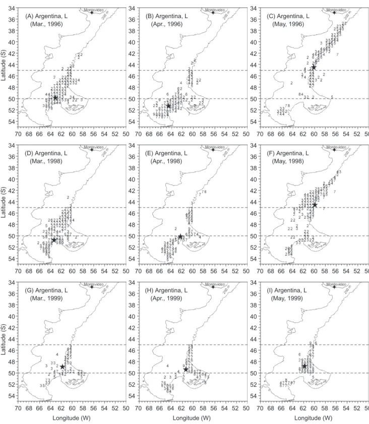
In ordinary years (1996 and 1998), we found that effects of month, latitude, and body size were significantly related to CPUE variations (p < 0.05), while the position on/off the shelf had no significant effect (Table 2). Body size and latitude explained substantial amounts of CPUE variations (p < 0.001), and 4 interaction terms of body size with latitude and being on/off the shelf, and month with body size and being on/off the shelf were signifi-cant in the model. In an ordinary year during Mar., the distribution of CPUE exhibited a continuous range with its highest value located in southern lat-itudes, and on average, the geographic center of biomass was located at 50
°
-51°
S, 63°
-64°
W (Fig. 4A, D). In Apr., the distribution map was divided into 2 ranges with 2 high CPUE centers, one directed toward the north and the other toward the south Fig. 4B, E). However on average, the geographic center showed little difference com-pared to the previous month. The distributional pattern greatly changed in May, with the CPUE distributed to the northern latitudes along the shelf break and the estimated center being located at 44°
-45°
S, 60°
-61°
W (Fig. 4C, F).In the high-abundance year (1999), we found that latitude and body size significantly loaded on CPUE variations (p < 0.01), while month and posi-tion on the shelf had no significant effects (Table 3). The size effect loaded on the CPUE was much greater than that of latitude. Moreover, the interac-tion of month x size had a synergistic effect com-pared to the effects individually. It is interesting that the effect of latitude x size was minor as shown in the final model by its relatively small F-ratio. During Mar.-Apr., the geographic patterns of the large-sized CPUE of 1999 were quite similar to those of ordinary years, although both geographic gravity centers were located a little north of the southern margin of the middle latitudes at 48
°
-49°
S, 61°
-62°
W and 49°
-50°
S, 61°
-62°
W, respectively (Fig. 4D, E). In May, most of larger CPUE values remained in the middle latitudes cen-tered at 49°
S, 62°
W, and showed little sign of moving northward to reach the northern latitudes (Fig. 4F).Latitudinal patterns
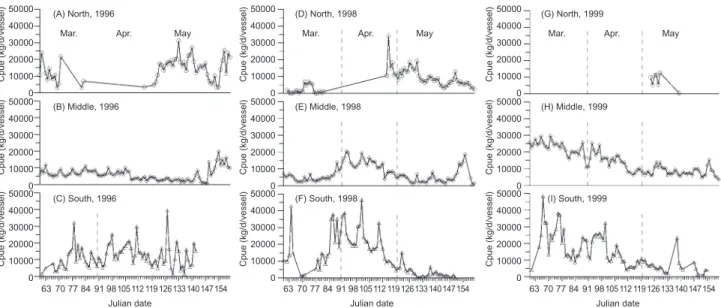
Within each latitudinal area, day-to-day changes in the CPUE are shown in figure 5. In ordinary years as illustrated by 1996 and 1998, in the northern latitudes, low CPUE values of less
Fig. 3. Cell-by-cell (0.5
°
-squared) differences in CPUE scores (a) between 1996 and 1999, and (b) between 1998 and 1999. A solid circle indicates that the subtracted CPUE score is positive, which means a higher abundance in 1999 than in 1996 or 1998. An open triangle indicates that the score is negative, which means a lower abundance in 1999 than in 1996 or 1998.34 36 38 40 42 44 46 48 50 52 54 Argentina (99-96) Latitude (S) Longitude (W) Montevideo 200 m 50 52 54 56 58 60 62 64 66 68 70 34 36 38 40 42 44 46 48 50 52 54 Argentina (99-98) Latitude (S) Longitude (W) Montevideo 200 m 50 52 54 56 58 60 62 64 66 68 70
than 20,000 kg/d/vessel were primarily found in early Mar., but by the end of Mar., no more fishing practices occurred until late Apr. and May when extensive fishing was again conducted (Fig. 5A,
D). In middle latitudes, relatively stable CPUE val-ues of about 10,000 kg/vessel/d began from the very beginning of Mar. and continued throughout the entire fishing season in both years, with a high
Fig. 4. Monthly distribution of CPUE (kg /d/vessel) estimated from large-sized squid in different years during Mar. and May (A-C for
1996, D-F for 1998, G-I for 1999). Numbers from 1 to 9 denote the following abundance levels: 0-2000, 2001-4000, 4001-6000, 6001-8000, 8001-10,000, 10,001-20,000, 20,001-30,000, 30,001-40,000, and > 40,000 kg /d/vessel. A star denotes the geographic locality of the gravity center weighted by abundance values.
Latitude (S) (A) Argentina, L (Mar., 1996) 50 52 54 56 58 60 62 64 66 68 70 34 36 38 40 42 44 46 48 50 52 54 Latitude (S) (D) Argentina, L (Mar., 1998) 50 52 54 56 58 60 62 64 66 68 70 34 36 38 40 42 44 46 48 50 52 54 Latitude (S) Longitude (W) (G) Argentina, L (Mar., 1999) 50 52 54 56 58 60 62 64 66 68 70 34 36 38 40 42 44 46 48 50 52 54 (B) Argentina, L (Apr., 1996) 50 52 54 56 58 60 62 64 66 68 70 34 36 38 40 42 44 46 48 50 52 54 (E) Argentina, L (Apr., 1998) 50 52 54 56 58 60 62 64 66 68 70 34 36 38 40 42 44 46 48 50 52 54 Longitude (W) (H) Argentina, L (Apr., 1999) 50 52 54 56 58 60 62 64 66 68 70 34 36 38 40 42 44 46 48 50 52 54 (C) Argentina, L (May, 1996) 50 52 54 56 58 60 62 64 66 68 70 34 36 38 40 42 44 46 48 50 52 54 (F) Argentina, L (May, 1998) 50 52 54 56 58 60 62 64 66 68 70 34 36 38 40 42 44 46 48 50 52 54 Longitude (W) (I) Argentina, L (May, 1999) 50 52 54 56 58 60 62 64 66 68 70 34 36 38 40 42 44 46 48 50 52 54
CPUE of 20,000 kg/d/vessel found in Apr. 1998 (Fig. 5B, E). In southern latitudes, different CPUE series were featured in 1996 and 1998: in the for-mer, values fluctuated around 10,000 kg/d/vessel from Mar. to May with several sporadic high catch-es of up to 30,000 kg/d/vcatch-essel, while the latter peaked at more than 30,000 kg/d/vessel during late Mar. and mid-Apr., in addition to high early catches in early-Mar. (Fig. 5C, F). Apparently, a
tapering trend after mid-April characterized the CPUE in 1998, while a fluctuating CPUE series was found in 1996.
In 1999, in the northern latitudes, no fishing was carried out during Mar.-Apr., with only a few days of fishing in May (Fig. 5G). In the middle lati-tudes, quite-high CPUEs (> 40,000 kg/d/vessel) began from early Mar., and gradually decreased to the end of May; nonetheless, values still remained
Fig. 5. Time-serial distributions of CPUE (kg/d/vessel) in northern, middle, and southern latitudes from 1 Mar. (the 60th Julian day) to
31 May (the 151st Julian day).
Table 2. Analysis of variance for log(CPUE) (kg/d/vessel), estimated from data of
Taiwanese jiggers in the Southwest Atlantic, on the effects of month, latitude, and body size in ordinary-abundance years (1996 and 1998)
Source of variation Sum of squares d.f. Mean square F-ratio Significance level Groupsa
Main effects 318.81 7 45.54 22.92 0.000
Month 13.08 2 6.54 3.29 0.038 (3, 5), (5, 4)
Latitude 67.67 2 33.84 17.03 0.000 2, (1, 3)
On/off the shelf 0.81 1 0.81 0.41 0.529 (1, 2)
Size 239.97 2 119.99 60.38 0.000 (1, 2), 3b Interactions 369.88 18 20.55 10.34 0.000 Month x latitude 14.62 4 3.65 1.84 0.119 Month x shelf 19.53 2 9.76 4.91 0.008 Month x size 31.75 4 7.94 3.99 0.003 Latitude x shelf 6.04 2 3.02 1.52 0.219 Latitude x size 133.40 4 33.35 16.78 0.000 Shelf x size 65.05 2 32.53 16.37 0.000 Residual 2514.03 1265 1.99 Total 3202.72 1290
aCategory codes are given in the remarks to table 1. bSize: 1, small (0.1-0.3 kg/ind); 2, median (0.3-0.4 kg/ind); 3, large (> (0.3-0.4 kg/ind).
50000 40000 30000 20000 10000 0 (A) North, 1996
Mar. Apr. May
Cpue (kg/d/vessel) 50000 40000 30000 20000 10000 0 (B) Middle, 1996 Cpue (kg/d/vessel) 50000 40000 30000 20000 10000 0 (C) South, 1996 Julian date 154 147 140 133 126 119 112 105 98 91 84 77 70 63 Cpue (kg/d/vessel) 50000 40000 30000 20000 10000 0 (D) North, 1998
Mar. Apr. May
Cpue (kg/d/vessel) 50000 40000 30000 20000 10000 0 (E) Middle, 1998 Cpue (kg/d/vessel) 50000 40000 30000 20000 10000 0 (F) South, 1998 Julian date 154 147 140 133 126 119 112 105 98 91 84 77 70 63 Cpue (kg/d/vessel) 50000 40000 30000 20000 10000 0 (G) North, 1999
Mar. Apr. May
Cpue (kg/d/vessel) 50000 40000 30000 20000 10000 0 (H) Middle, 1999 Cpue (kg/d/vessel) 50000 40000 30000 20000 10000 0 (I) South, 1999 Julian date 154 147 140 133 126 119 112 105 98 91 84 77 70 63 Cpue (kg/d/vessel)
at about 20,000 kg/d/vessel to the end of the sea-son (Fig. 5H). In southern latitudes, high CPUEs began from early Mar., and the value quickly increased up to > 40,000 kg/d/vessel in mid-Mar. The increases even soared to 90,000 kg/d/vessel in early Mar., but the values gradually dropped thereafter (Fig. 5I). It is apparent that daily catch rates in 1999 outnumbered those of ordinary years on an almost daily basis at all fishing sites in the middle and southern latitudes.
Body size changes
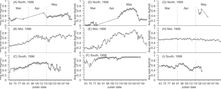
Within each latitudinal area, day-to-day aver-age size changes are illustrated in figure 6. In the ordinary years of 1996 and 1998, in northern lati-tudes, the initial body size was about 0.2 kg/ind or smaller in early Mar., and various sizes ranging from 0.2 to > 0.6 kg/ind were found in May (Fig. 6A, D). In middle latitudes in 1996, small-sized squid (~0.3 kg/ind) increased in weight from Mar. to the end of Apr., reaching a size exceeding 0.6 kg/ind, but the size dropped a bit during late-Apr. and early May, going up again after that (Fig. 6B). In the same period, the size of squid in 1998 steadily increased from late Mar. (0.2 kg/ind) to mid-May (0.8 kg/ind), and then decreased after mid-May (Fig. 6E). In southern latitudes, the body size increased to more than 0.6 kg/ind after late Mar., but the average size dropped slightly after Apr. in 1996 (Fig. 6C), while the size remained quite large throughout the 1998 fishing season
(Fig. 6F). It turns out that during May squid of all sizes ranging from small (0.2-0.4 kg/ind), median (0.4-0.5 kg/ind) to large (> 0.5 kg/ind) occurred in middle latitudes, and squid of median-large size (0.4-0.6 kg/ind) turned north beginning in early May. In 1999 in northern latitudes, median to large squid only occurred in May (Fig. 6G). In middle latitudes, squid sized 0.6 kg/ind uniformly occurred almost throughout the entire season (Fig. 6H). In southern latitudes, squid of slightly less than 0.6 kg/ind recurrently appeared until early May. It is obvious that large squid exceeding 0.8 kg/ind were rarely found in the 1999 fishing season, and also in southern latitudes, the size in 1999 was almost always less than that of ordinary years (Fig. 6C, F vs. 6I).
Temperature variations
The mean in situ water temperature at fishing sites with a high CPUE is shown in table 4. The most significant in situ temperature difference was in the northern latitudes during May: in 1999, the water (9.00
°
C) was colder than in ordinary years (11.83 and 11.43°
C for 1996 and 1988, respective-ly) with 100% bootstrap probability. In addition, during the previous month of Apr. further south at locations in the middle and southern latitudes, tem-perature differences were also obvious; bootstrap statistics showed that 89% of the possibility sup-ports the middle-latitude water temperature (9.93°
C) in 1999 being colder than usualTable 3. Analysis of variance for log(CPUE) (kg/d/vessel), estimated from data of
Taiwanese jiggers in the Southwest Atlantic, on the effects of month and body size in a high-abundance year (1999)
Source of variation Sum of squares d.f. Mean square F-ratio Significance level Groupsa
Main effects 107.30 7 15.33 12.94 0.000
Month 5.10 2 2.55 2.15 0.118 (3, 4, 5)
Latitude 13.49 2 6.74 5.69 0.004 (3, 1), (2,1)
On/off the shelf 0.30 1 0.30 0.25 0.621 (1, 2)
Size 91.97 2 45.99 38.80 0.000 1, 2, 3 Interactions 237.34 12 19.78 16.69 0.000 Month x shelf 10.37 2 5.19 4.37 0.013 Month x size 193.72 4 48.43 40.87 0.000 Latitude x size 23.76 4 5.92 4.99 0.001 Shelf x size 4.35 2 2.17 1.83 0.161 Residual 469.30 396 1.19 Total 813.94 415
(10.11
°
C and 10.79°
C); however, the temperature differences decreased in more-southerly latitudes because only a marginal possibility (65%) sup-ports the 1999 temperature (8.63°
C) being colder than ordinary (9.81°
C and 9.01°
C). Apart from that, in northern latitudes, within-group variations were also found to be smaller (with a coefficient of variation (CV) of 5.78%) in May of 1999, in con-trast to ordinary years (13.16%) in northern lati-tudes. The low within-group variations in tempera-ture indicate that a uniformly colder water mass existed in 1999.DISCUSSION
The current study provides the first detailed description of the abundance patterns and size structures of the Argentine squid from large-scale fisheries data over low-, median-, and high-yield years. This study also analyzed the sources of variations over an environmental gradient extend-ing from low (subtropical) to high (sub-Antarctic) latitudes. As the presumptions that we set forth, annual differences became the most influential effect contributing to CPUE variances in the GLM, but it turned out that only 2 groups of ordinary- and high-abundance contrasts significantly differed statistically. By hierarchical design to remove the annual effect, latitudinal differences were the next significant factor (Tables 1-3), and accordingly, the latitude effect was further interpreted by the envi-ronmental factor of in situ water temperature.
Spatiotemporal changes
In ordinary years (1996 and 1998), our find-ings on the spatiotemporal distribution patterns of CPUE fairly support the present available migra-tion models for Argentine squid in the Southwest Atlantic. First of all, the fact that our catch dataset was retrieved in the peak fishing season (Mar.-May) may correspond to the most-abundant winter cohort of Argentine squid as summarized by Haimovici et al. (1998). This is also evidenced by statolith readings, and then back-estimated to obtain their hatching dates in the austral winter (Chen et al. 2002). Our results of the monthly spatial distribution of the CPUE based on large-sized squid (> 0.4 kg/ind) is in agreement with pre-vious studies of the pre-spawning winter cohort (Brunetti et al. 1998, Haimovivi et al. 1998); as shown by 3 successive monthly abundance pat-terns in ordinary years: 1) a continuous population range with high abundances heading to southern latitudes on the outer Patagonian Shelf in Mar. (Fig. 4A, D); 2) subsequently a divided range with 2 high abundance centers, one directed toward the north and the other toward the south in Apr. (Fig. 4B, E); and 3) thereafter a major concentra-tion of squid located in the northern latitudes, with several remnants scattered in middle and southern latitudes in May (Fig. 4C, F). During Mar. and Apr., squid of < 0.6 kg/ind in northern and middle latitudes (Fig. 6) are thought to engage in a feed-ing migration (Arkhipkin 2000), and are distributed over southern Patagonian Shelf waters, which are
Fig. 6. Time-serial distributions of average body size (kg/ind) in northern, middle, and southern latitudes from 1 Mar. (the 60th Julian
day) to 31 May (the 151st Julian day).
1 0.8 0.6 0.4 0.2 0 (A) North, 1996 Mar. A vg size (kg/ind) Apr. May 1 0.8 0.6 0.4 0.2 0 (B) Mid, 1996 A vg size (kg/ind) 1 0.8 0.6 0.4 0.2 0 (C) South, 1996 A vg size (kg/ind) 1 0.8 0.6 0.4 0.2 0 (D) North, 1998 Mar. A vg size (kg/ind) Apr. May 1 0.8 0.6 0.4 0.2 0 (E) Mid, 1998 A vg size (kg/ind) Julian date 1 0.8 0.6 0.4 0.2 0 (F) South, 1998 A vg size (kg/ind) 1 0.8 0.6 0.4 0.2 0 (G) North, 1999 Mar. A vg size (kg/ind) Apr. May 1 0.8 0.6 0.4 0.2 0 (H) Mid, 1999 A vg size (kg/ind) 1 0.8 0.6 0.4 0.2 0 (I) South, 1999 A vg size (kg/ind) 154 147 140 133 126 119 112 105 98 91 84 77 70 63 Julian date 154 147 140 133 126 119 112 105 98 91 84 77 70 63 Julian date 154 147 140 133 126 119 112 105 98 91 84 77 70 63
enriched by subsurface flows of the Patagonian or Falkland (Malvinas) Current. During May, the dis-tribution pattern of large-sized squid shifts north-ward (Figs. 4C, F, 6B, E), and the range of squid extend to the north of 40
°
S, approximately reach-ing the confluence area of the cold Falkland (Malvinas) and the warm Brazil Currents at about 38°
S (Fig. 1, Garzoli and Garraffo 1989). However, it is also apparent that in 1999, large-sized pre-spawning squid (> 0.4 kg/ind) were not found to the north of 44°
S, but rather we found a concentrated population centered at 49°
S, 62°
W (Fig. 4I). This discordant distribution pattern trig-gered an extended fishing season with a high CPUE in middle latitudes (Fig. 5h), and might be linked to the causes of the high catches in 1999 (Fig. 2).Characteristics of high abundance
To incorporate biomass (kg) into the CPUE to represent abundances of Argentine squid, the dynamic nature of body size changing from month to month should stringently be taken into account. Argentine squid are a semelparous species with a short life of about 1 yr, but they grow fast during their lifespan in the Southwest Atlantic including around the Brazil and Falkland (Malvinas) Currents (Rodhouse and Hatfield 1990, Rodhouse et al. 1995). As to the average size of squid in the Southwest Atlantic, through the GLM analysis, body size and latitude explained most of the CPUE variations, and this pattern was also significant
when the effect of 2nd-order interactions were included in the model (Table 2). In ordinary years, large squid (> 0.6 kg/ind) were first found in south-ern latitudes in Mar. or Apr. (Fig. 6C, F), and were later found in middle latitudes (Fig. 6B, E). The squid were found to have gained weight while in the southern latitudes, generally reaching a large size exceeding 0.6 kg/ind after mid-Apr. Some squid had already shifted northwards in May, but the size apparently did not further increase (Fig. 6A, B). In 1999, CPUE values showed very signifi-cant intra-annual variations on a daily basis (Figs. 5G-I), which were interactively affected by varia-tions in body size and latitude (Table 3). As shown by the multiple-range tests and temporal distribu-tion patterns (Figs. 6G-I), the initial size of squid in early Mar. 1999 was generally quite large at around 0.5-0.6 kg/ind compared to ordinary years; however, this size did not increase but rather slightly decreased in southern latitudes (Fig. 6I). In southern latitudes, the pattern of relatively smaller sizes after Apr. 1999 than ordinary was intriguing to us, and we made several supposi-tions, such as 1) size selection by the jigging equipment, 2) size-segregated migration, i.e., large squid had emigrated and small squid had immi-grated, or 3) even ontogenetic energy partitioning as they appeared in the fishing ground. Size selection by jigs is difficult to assess (Millar and Fryer 1999), but differences in gear selectivity among years are unlikely, because no significant changes in fishing gauges or methods are known to have occurred during our study period. Different
Table 4. Mean in situ water temperatures from high-CPUE (represented by
upper quartile values) fishing sites in the Southwest Atlantic
Latitude Year Water temperature (
°
C) measured at 5 m in depthMar. Apr. May
North 1996 12.53 ± 1.41a - b 11.83 ± 2.00 1998 13.17 ± 0.47 - 11.43 ± 1.06 1999 - - 9.00 ± 0.52 Mid 1996 11.48 ± 1.25 10.11 ± 1.19 9.05 ± 1.04 1998 12.73 ± 1.00 10.79 ± 0.91 10.25 ± 1.01 1999 12.03 ± 1.01 9.93 ± 0.77 9.03 ± 0.90 South 1996 10.18 ± 1.10 9.81 ± 1.45 -1998 9.72 ± 1.07 9.01 ± 1.23 9.58 ± 1.08 1999 9.45 ± 0.79 8.63 ± 0.59 8.50 ± 0.70
aStandard deviation estimated across the daily average. bIndicates that data were unavailable from the fishing practice.
gear selectivity between latitudes, such as middle and southern latitudes, possibly occurring within a year (1999) is also at odds with reality, because the fleet in 1999 was composed of the same jigger vessels as in ordinary years. For a life cycle vari-able of ommastrephid species, the interaction between life history strategies and oceanographic conditions should affect various demographic traits, such as growth and maturation (Markaida and Sosa-Nishizaki 2001, McGrath and Jackson 2002, Pecl et al. 2004). By rule of thumb, much fewer large-sized squids but a rather large number of median-sized squid (0.5-0.6 kg/ind) were caught almost throughout 1999 (Figs. 6G-I), indicating that a large portion of individual squid did not effective-ly grow to a larger size of greater than 0.6 kg/ind compared to ordinary years. Unfavorable oceano-graphic conditions, such as low temperatures, could have caused the small-sized squid found in 1999; however, biological factors might also have caused smaller body sizes, such as density-dependent effects or higher competition for food. Further details should be investigated before answers are possible. At this moment, annu-al variations in sea water temperature are an inter-esting clue.
Sea water temperature links to high abun-dances
Regarding the favorite water temperature recorded with high CPUE values from Mar. to May in the Southwest Atlantic, its decrease was fairly similar within each latitudinal area over ordinary years, but apparently a cold sub-surface water temperature was found in May 1999 (9.0
°
C vs. 11.43°
C of 1998 and 11.83°
C of 1996, Table 4). In May, the squid begin to adjust from juveniles to the pre-spawning stage. If relatively little heat was retained in the waters of the northern latitudes of the Patagonian Shelf, the squid might not have been able to grow to an ordinary size of more than 0.6 kg/ind after Apr. (Figs. 6G-I), resulting in a pro-tracted pre-spawning migration to northern lati-tudes. The delayed movement is shown by a pat-tern of low to almost no occurrence of squid in northern latitudes during May 1999 (Figs. 4I, 5G). An overextended somatic development period of squid would mean a smaller reproductive invest-ment, which is in agreement with a larger amount of standing biomass but rather-small individual sizes as shown by the highest annual catches in 1999. Nonetheless, we should not rule out other possibilities, such as 1) continuous recruitmentfrom uncommon resources which were thus encountered by the fishery, and 2) large rations and a favorable feeding environment for the squid. Many researchers have established the distribution and abundance patterns of the Argentine squid in Southwest Atlantic waters, and have also offered possible mechanisms for fluctuations in abun-dances (Rodhouse et al. 1995, Waluda et al. 1999 2001a b) that may also provide clues to explain the causes of high abundances or catches. At hatch-ing sites, larval mortality may have profound effects on the subsequent recruitment strength, and at feeding and nursery grounds, distribution patterns may affect catch rates in the exploitation phase. Waluda et al. (1999) reported that the recruitment strength of Argentine squid reacted negatively to sea surface temperature (SST) val-ues at its hatching site, but on the other hand, commercial catches of squid were negatively relat-ed to the areal extent of the frontal zone, and posi-tively related to that of favorable SSTs (Waluda et al. 2001a). In terms of the fishing grounds, marine conditions, such as water thermal fronts, may affect the distribution patterns of squid and thus be reflected in fishery catches; for example, high CPUE values were matched with a zone of high SST gradients (Waluda et al. 2001b). This may be helpful in explaining the high production rates of 1999 in the middle latitudes where entrapment of pre-spawning squid was identified (Figs. 4I, 5H). In this study, we have clearly elucidated various patterns of abundance and movements of Argentine squid with detailed analyses of jigging catch records, and explained that variations in the distribution, movement, catch rates, and body size of the squid depend to a considerable degree on changes of thermal conditions in the Southwest Atlantic.
Acknowledgements: The authors are indebted to
the Overseas Fisheries Development Council of the R.O.C. for collection and maintenance of log-book data. We thank 2 anonymous reviewers for kindly offering insightful comments that improved our manuscript. Financial support was provided, in part, through a project from the Fishery Agency, Council of Agriculture, R.O.C. Thanks are also extended to an assistant on the project, Ms. K.Z. Chang, for help in conducting the project.
REFERENCES
and variability: ommastrephid squid in the variable oceanography environments. Fish. Res. 54: 133-143. Anonymous. 2004. FAO yearbook. Fishery statistics
-Capture production 2002. Vol. 94/1. Rome: Food and Agriculture Organization.
Arkhipkin AI. 2000. Intrapopulation structure of winter-spawned Argentine shortfin squid, Illex argentinus (Cephalopoda, Ommastrephidae), during its feeding peri-od over the Patagonian Shelf. Fish. Bull. (US) 98: 1-13. Basson M, JR Beddington, JA Crombie, SJ Holden, LV
Purchase, GA Tingley. 1996. Assessment and manage-ment techniques for migratory annual squid stocks: the
Illex argentinus fishery in the Southwest Atlantic as an
example. Fish. Res. 28: 3-27.
Beddington JR, AA Rosenberg, JA Crombie, GP Kirkwood. 1990. Stock assessment and the provision of manage-ment advice for the short fin squid fishery in Falkland Islands waters. Fish. Res. 8: 351-365.
Brunetti N, ML Ivanovic. 1992. Distribution and abundance of early stages of squid (Illex argentinus) in the southwest Atlantic. ICES J. Mar. Sci. 49: 175-183.
Brunetti N, M Ivanovic, G Rossi, B Elena, S Pineda. 1998. Fishery biology and life history of Illex argentinus. In T Okutani, ed. Contributed papers to International Symposium on Large Pelagic Squid. Tokyo: Japan Marine Fishery Resources Research Center (JAMARC), pp. 217-232.
Chen CS, MS Shiao, TS Chiu. 2002. Growth of Argentine shortfin squid, Illex argentinus, in the southwest Atlantic during its post-recruitment migration. Acta Oceanogr. Taiwanica 40: 33-46.
Garzoli SL, Z Garraffo. 1989. Transports, frontal motions and eddies at the Brazil-Malvinas currents confluence. Deep-Sea Res. Part A Oceanogr. Res. Pap. 36: 681-703. Haimovici M, NE Brunetti, PG Rodhouse, J Csirke, RH Leta.
1998. Illex argentinus. In PG Rodhouse, EG Dawe, RK O,Dor, eds. Squid recruitment dynamics. The genus
Illex as a model, the commercial Illex species and
influ-ence on variability. FAO Fisheries Technical Paper no. 376. Rome: Food and Agriculture Organization, pp. 27-58.
Hatanaka H. 1986. Growth and life span of short-finned squid
Illex argentinus in the waters off Argentina. Bull. Jpn.
Soc. Sci. Fish. 52: 11-17.
Hatanaka H. 1988. Feeding migration of short-finned squid
Illex argentinus in the waters off Argentina. Nippon
Suisan Gakk. 54: 1343-1349.
Hilborn R, CJ Walters. 1992. Quantitative fisheries stock assessment: choice, dynamics and uncertainty. New
York: Chapman and Hall.
Leta HR. 1992. Abundance and distribution of Illex argentinus rhynchoteuthion larvae (Cephalopod, Ommastrephidae) in the waters of the southwestern Atlantic (Argentine-Uruguayan common fishing zone). S. Afr. J. Mar. Sci. 12: 927-941.
Manly BFJ. 1997. Randomization, Bootstrap and Monte Carlo methods in Biology. London: Chapman and Hall. Markaida U, O Sasa-Nishizaki. 2001. Reproductive biology of
jumbo squid Dosidicus gigas in the Gulf of California, 1995-1997. Fish. Res. 54: 63-82.
McGrath BL, GD Jackson. 2002. Egg production in the arrow squid Nototodarus gouldi (Cephalopoda: Ommastre-phidae), fast and furious or slow and steady? Mar. Biol.
141: 699-706.
Millar RB, RJ Fryer. 1999. Estimating the size selection curves of towed gears, traps, traps, nets and hooks. Rev. Fish Biol. Fisher. 9: 89-116.
Pecl GT, NA Motschaniwskyj, SR Tracey, AR Jordan. 2004. Inter-annual plasticity of squid life history and population structure: ecological and management implications. Oecologia 139: 515-524.
Rodhouse PG. 2001. Managing and forecasting squid fish-eries in variable environments. Fish. Res. 54: 3-8. Rodhouse PG, J Barton, EMC Hatfield, C Symon. 1995. Illex
argentinus: life cycle, population structure, and fishery.
ICES Mar. Sci. Symp. 199: 425-432.
Rodhouse PG, EMC Hatfield. 1990. Dynamics of growth and maturation in the cephalopod Illex argentinus de Castellanos, 1960 (Teuthoidea: Ommastrephidae). Philos. T. Roy. Soc. B 329: 229-241.
Rosenberg AA, GP Kirkwood, JA Crobie, JR Beddington. 1990. The assessment of stocks of annual squid species. Fish. Res. 8: 335-350.
Salthaug A, OR Godø. 2001. Standardization of commercial CPUE. Fish. Res. 49: 271-281.
Waluda CM, PG Rodhouse, GP Podesta, PN Trathan, GJ Pierce. 2001a. Surface oceanography of the inferred hatching grounds of Illex argentinus (Cephalopoda: Ommastrephidae) and influences on recruitment variabili-ty. Mar. Biol. 139: 671-679.
Waluda CM, PG Rodhouse, PN Trathan, GJ Pierce. 2001b. Remotely sensed mesoscale oceanography and the distri-bution of Illex argentinus in the South Atlantic. Fish. Oceanogr. 10: 207-216.
Waluda CM, PN Trathan, PG Rodhouse. 1999. Influence of oceanographic variability on recruitment in the Illex
argentinus (Cephalopoda: Ommastrephidae) fishery in the