Please cite this paper as follows:
H.-K. Hong and J.-K. Liou, Integral-Equation Representations of Flow Elastoplasticity Derived from
Rate-Equation Models, Acta Mechanica, Vol.96, pp.181-202, 1993.
Acta Mechanica 96, 1 8 1 - 2 0 2 (1993)
ACTA MECHANICA
'~ Springer-Verlag 1993Integral-equation representations of flow
elastoplasticity derived from rate-equation models
H . - K . H o n g , Taipei, a n d J . - K . Liou, T a o y u a n , T a i w a n
(Received May 21, 1991; revised September 16, 1991)
Summary. Two integral-equation representations are presented in this paper, based on the exact integrations of the conventional rate-equation model of associative J2 flow elastoplasticity with com- bined-isotropic-kinematic hardening-softening. Among them the strain-controlled integral-equation repre- sentation has two new naturally defined material functions Y(Z) and U(Z) of the normalized active work Z, which plays the role of intrinsic time. One of the immediate benefits derivable from the new representations is, owing to the explicit unfolding of the highly nonlinear path-dependence between stress and strain without a detour to the evolutions of internal state variables, their adaptability for direct calculations without any iteration. Indeed, it is itself a constructive algorithm. It is shown that at a realistic level of precision, the strain-controlled integral-equation representation saves 99% or more of the C P U time compared with the widely used elastic predictor-radial return algorithm of the rate-equation representation.
List of symbols
eli, e~j, e,~gp el, e2,e3 etan, erad E f F G G(Z1, Z2) h(~), k(~) H(~r), K(g9 12 J(z~, z9 Yf p rlj R~j s,, s~j, s~ g,. Sl~ $2, $3
strain deviator, elastic strain deviator, piastic strain deviator effective strain
effective plastic strain
principal strain deviator, e3 = - e l - e 2
tangential strain increment, radial strain increment Young's modulus, assumed to be constant yield function in stress space
yield function in strain space
shear modulus, assumed to be constant shear relaxation function of elastoplasticity
material functions of plasticity for the stress-space rate-equation representation material functions of plasticity for the strain-space rate-equation representation second invariant of the deviatoric strain tensor
second invariant of the deviatoric stress tensor shear creep function of elastoplasticity bulk modulus, assumed to be constant
dummy variable of integration in place of the effective plastic strain active stress
active strain
effective active-stress, i.e. 3 ~ times Euclidean length of active stress effective active-strain, i.e. ] / ~ times Euclidean length of active strain stress deviator, elastic stress deviator, stress relaxation
effective stress
effective stress relaxation
182 H.-K. Hong and J.-K. Liou to t. y(z), u(~) r(z), u(z) 2
e(e;), ;(e;), a(e;) z o~ij A~j e v ~ij~ glj, g~j gy V
ffij, (Tiej, (7i 5 ay
time
zero-value time latest unloading time
material functions of plasticity for the stress-controlled integral-equation representation material functions of plasticity for the strain-controlled integral-equation representation normalized active complementary-work
material functions defined for use in converting h(6 p) and k(~ p) to y(z) and u(z) normalized active work
material functions defined for use in converting h(g p) and k(g p) to Y(Z) and U(Z) back stress
back strain
strain, elastic strain, plastic strain (initial) yield strain, gy = h(O)/2G Poisson's ratio, assumed to be constant stress, elastic stress, stress relaxation (initial) yield stress, yield strength, cry = h(0)
1 Introduction
The formulation of the yield criteria of Tresca (1870) and von Mises (1913) was the first key step in developing plasticity theory. However, without a plastic stress-strain relation, the criteria can do little. The incremental stress-strain relations proposed by St. Venant (1870) and Levy (1870) represented a giant step forward in plasticity theory. Since then the incremental- or rate-type point-of-view has been most frequently taken in formulating constitutive equations of plasticity, which describe the evolutions of internal state variables. This kind of rate-equation representations is now composed of separately specified but interwoven ingre- dients, including the elastic part, yield criterion, loading condition, plastic flow rule and hardening rule.
To this rate-equation point-of-view and model, the usual analysis approaches require numerical integrations of the incremental or rate equations over a discrete sequence of steps, keeping the plastic strain increment n o r m a l to the evolving yield surface at each step, meanwhile managing to attach the current stress state on the current yield surface, which is moving and deforming in stress space in a way corresponding back to the plastic strain increment in the plastic strain space. Because of the interwoven nature of the model ingredients, the difficulties involved and its great consumption of computational time, and the efficiency and accuracy of the global solutions of structural and mechanical problems being strongly influenced by the efficiency and accuracy of constitutive-equation solving schemes, it has drawn much attention over the past 25 years and has directed m a n y efforts spent in this issue aiming at developing accurate and economic algorithms [1] - [4]. However, owing to the great difficulties rooted in the very nature of this highly nonlinear path-dependence problem, thorough solutions have still been pending.
In this paper, the rate equations are exactly integrated and then new material functions are so naturally defined that two new integral-equation representations are established to model the same behavior of flow elastoplasticity. As consequences, calculations are much easier and new viewpoints at the flow elastoplasticity are emerging. A total of four representations are addressed in the paper. They are the conventional stress-space rate-equation representation, the strain-space rate-equation representation, and the new strain-controlled and stress-controlled integral-equation representations.
Integral-equation representations of flow elastoplasticity 183
2 Stress-space rate-equation representation
We confine ourselves to the following material of flow elastoplasticity, which can be modeled by either a stress-space or a strain-space representation, both expressed in the form of rate equations. In the stress-space representation, the yield fuction
f - f - h((p) < 0 (1)
is defined on stress space and strain is postulated to be composed of two parts:
~ij = s~j + ~ , (2)
in which the elastic part is governed by
1 1
c.e ,, = ~ Sij, ,~e kk = y y ~ l , (3)
and the plastic part is governed by the evolution rules for the back stress c~i~ and the plastic strain
p
e~j respectively, i.e. 2
d:,j = ~ k'(g p) d~, C~kk = O, (4)
c?f = e p 3 e.
~ = ~ , ~ ~ ~,~, ~ = 0, (5)
in which e p is implicitly defined and further required to conform to
{ 21
> 0 if f = h and r~jgij = ~ - (h + k),
e v (6)
= 0 otherwise,
where f = h, i.e.,f = 0 is the yield condition in stress space and r~j~i~ = (/~ +/~) 2h/3, i . e . , f = 0 is the straining condition for the stress-space rate-equation representation, which replaces the role of the conventional loading condition.
As usual, a~j is the stress, e~j is the strain, s~j is the stress deviator, e~j is the strain deviator,
r i j = S i j - - O~ij (7)
is the active stress and
= r~ r ~ ) (8)
is the effective active-stress, always < h(6P). A superimposed dot stands for the material time differentiation and a function of one argument with prime superscript denotes the derivative of the function with respect to the argument. The superscripts e and p signify respectively the elastic and plastic parts. F r o m Eqs. (5) and (6),
184 H.-K. Hong and J.-K. Liou and the effective plastic strain 8P is
8P = i eP(r) dz,
(10)to
that is 2 ~ times the arc length of the path travelling in the plastic strain space.
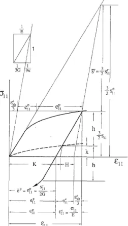
It is postulated that there exists conceptually the zero-value (or virgin or free) state at th~ zero-value time, to, when all relevant values vanish. Accordingly, the model is general enough to deal with the problems of nonzero initial values if the initial conditions of the stress, strain, back stress and effective plastic strain are known. In particular, initial isotropy of plastic response, which is u n c o m m o n in practice and can be achived in laboratories only through the greatest of care in the preparation of the material and in the fabrication of the test specimen (Drucker [5]), is not assumed at all. Small deformation is assumed throughout in the present paper. As a consequence, Eqs. (2), (3) and (7) are written directly in total forms. The model of the material under consideration employs the yield criterion of the von Mises type (Eq. (1)), and the normality law of plastic flow (Eq. (5)) with the hardening-softening rule of the Prager type (Eq. (4)) or the Ziegler type (Eqs. (5) into (4)); the two rules are identical in the context of the present paper. Constants and functions of material properties employed include the bulk modulus X (or Poisson's ratio v or Young's modulus E), shear modulus G, and yield-stress function of material h(Y p) and back-stress function of material k(FP). The elastic moduli X (or v or E) and G are assumed to be constant. To determine the material functions, h(Y p) and k(YP), we m a y perform a uniaxial stress (tension or compression) test for h + k, and a series of reserved yieldingtests for k - h, in which loads are added up to different stress levels over the first-time yield and then
8"11
Fig. 1. Relations of material constants and functions in the stress- and strain-space representations determined from a uniaxial stress (tension or compression) test and a series of reversed yielding tests
Integral-equation representations of flow elastoplasticity 185
(Y12 = S12
e12=e12
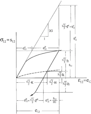
Fig. 2. Relations of material constants and functions in the stress- and strain-space re- presentations determined alternatively from a test of a thin-walled circular tube under monotonic torque and a series of reversed yielding tests
released and reversed until another yields take place in the opposite sense, the relations of these material functions and constants being schematically illustrated in Fig. 1. Alternatively, a test of a thin-walled circular tube under m o n o t o n i c torque, for h + k, and a series of reversed yielding torsion tests, for k - h, can also be employed to determine
h(~ p)
and k(~P), the relations of these material functions and constants being schematically shown in Fig. 2.It is important to note that in Eq. (6) the straining condition is written as 2h
rijgij
= ~ (/~ +/~), (11)the necessary and sufficient condition of which is
f = 0. (12)
If the cases of hardening, perfect, and softening plasticity are distinguished according to the sign of h' + k', that is the slope of the stress-plastic strain curve of the uniaxial stress or tube-twisting test, the straining conditions for them can be respectively written as
2h { > 0
r~j~j = ~ - (h' + k') e p = 0 < 0 .
(13)
Caution that it is ambiguous to address only on the sign
rijSij
without mentioning the equality ofrljgij
and (/~ +/~)2h/3,
since although, for permissiblesij, rij~ij
> 0 means straining and loading,rijg~j
= 0 m a y also mean straining and neutral loading for perfect plasticity, whiler~j&j
< 0 m a y as well a c c o m p a n y straining for softening plasticity or m a y as usual mean unloading and unstraining.It is reminded that g~j here in Eq. (11) more or less suggests, if does not mandate, that ~ij or
d&j
186 H.-K. Hong and J.-K. Liou
suitable for situations where the strain-increment response to a prescribed stress-increment is to be sought. However, s~j and g~j are not always permissible, the path in stress space being constrained when the material is perfectly plastic or softens; r~j~ij can only be negative for softening plasticity and is not allowed greater than zero for perfect plasticity. Moreover, a strict stick to the stress control fails for softening plasticity, since stress alone cannot determine uniquely if it strains or unstrains, manifested most clearly in real-world material tests. On the contrary, strain can, for the material investigated, control the material response. This p h e n o m e n o n inherently associated with the stress control of softening-plastic materials is called material indeterminacy. Resort to coupling with other physical laws or a shift to the strain control is inevitable [6]. Although the stress-space rate-equation representation is m o r e suited to the stress control, it is still very frequently used in strain-controlled formulations, notable examples including m a n y finite element stiffness procedures. It is therefore felt that the straining condition for the stress-space rate-equation representation m a y be tradeoff specified a s f = 0 or r~j~j = (/~ +/~)2h/3, in order that it can be used independently of whether the material workhardens, is perfectly plastic, or worksoftens, with the understanding of the material indeterminacy haunted by the situation mentioned. Nevertheless, if the material or the range considered is all the way hardening, the straining condition is simply meanwhile much more tractably specified as rlj~ij > 0. Besides, it is noted that the straining and the straining condition as used herein m a y include the so-called "neutral" ones and that the c o m m o n usage of the stress-space rate-equation representation under the strain control renders such implicit algorithms that do complicate calculations.
3 Integration of rate equations given a strain history
N o w we proceed to the main issue of integrating the constitutive rate equations of the above model to integral equations when a strain history is given and the yield and straining conditions are satisfied. F r o m Eqs. (2) and (3),
sij = 2Ge~j = 2Geij - 2Ge~. (14)
Substituting Eqs. (7), (4) and (14) into the identity
(slj - &i j) + c~ij = gij (15)
yields 2
?,j + ~ k'd~ = 2Gd,j - 2GO~, (16)
which, upon considering Eq. (5) and f - f - h = 0, becomes
k ' + 3 G .
t'ij + ~ 6Prlj = 2Gd~j, (17)
o r
Integral-equation representations of flow elastoplasticity 187 where
"Y(gP) -= exp
k'(p) + 3G dp
h(p)
(19)
is a material function. In this paper, for clarity, p symbolizes a dummy variable of integration in place of the effective plastic strain YP. Eq. (17) is an ordinary differential equation for the active stress tensor, the solution of which can be readily written as
rid(t)
1
2G
~FP(t))
f(e~(z)) r,(z)
2G- + Y(~(~)) ode) de .
f
(20) Again from Eq. (17),~P
furl1 + (k' +
3G) ~-ri~r u = 2GOur u.
(21)When the yield condition f = 0 and the straining f = 0 are satisfied,
2 2
ri~rij = ~ h 2,
r
= ~ hh'~ p.
(22)Substitution of Eqs. (22) and (20) into Eq. (21) yields
4G2eid(t ) [
rid(r)
23 hh'eP +
(k' +
3G)ePh - f(Fp(t)) Y(e-P(z)) ~ -
+ f ?(e~(~)) O'd(~)
d~ 1'
which is then multiplied by
f(YP(t))/4G 2
and rearranged to give(23)
h ' + k ' + 3 G
6G 2
hf(gP(t)) e p = !7(F'(r))~u(t)~ + ~u(t) f f(FP(~))eu(~)d~.
1: (24) Define ~p
2(Fp ) _ f h'(p) +6G 2k'(p) + 3G
oh ' + k ' + 3 G
h(p) Y(p) dp,
Z' -
h f z,
(25)6G 2
h' k'Z(t) =-
2(yP(t)), 2(0 = 2(gP(t)) = 2 ' e p - + + 3G h!Tep. (26) 6G 2Note that 2(~ p) is a material function while Z(0 and eP(t) are merely functions of time. From Eqs. (24) and (26),
z(t)
= z(~) + ep(z)) ~,j(r T d -r
188
or, after interchanging the order of integrations,
t
r~j(~) f
Z ( t ) = Z(z) +
1?(eP(~))
[eu(t ) -eu(~)] 2G +
I~(6P(~)) [eu(t) - eu(r ~u(r de.
Next, Eq. (5) can be integrated:
i 3eP(~)
e~(t) = e~(z) + 2 ~ ) ) ru(~) d~.
Combination of Eqs. (14), (29) and (20) yields
f
i 3eP(~) 2Gsu( 0 = su(~ ) + 2G eu(t ) e u ( z ) - 2 ~ ) ) f(YP(~))
l
_ _ r , s;
It
•
r(ep(~)) Td- +
P(~(0) ~,j(0 d~ d~
z Define ~p 0(6~') = 3GY(SP) h(p) Y(p)' 0H.-K. Hong and J.-K. Liou
(28)
(29)
(30)
(31)
which is a material function. Interchanging the order of integrations in Eq. (30) and using definition (31) and once again Eq. (20), we have
- 8(~p(t)) ~dt)
T8-
+
8(v'(~))
~d~)
5 8
+
i
[1
z
+ 8(~(0)] o,j(~) d~}.
su(t ) = su@ ) + 2G (32)
Thus far the expressions for ru, Z and s u in the form of integral equations are available.
4 Strain-controlled integral-equation representation
A careful examination of the integral equations derived above leads us to recognize the important role Z plays in developing a new perspective at the flow plasticity that instead of
the rate-equation representation with the material functions h(g p) and k(8 p) of O p, we may
propose an integral-equation representation with material functions Y(Z) and U(Z) of Z, as
defined by
(YZ) =- g ( z l ( Z ) ) : Y ( e P ) , (33)
integral-equation representations of flow elastoplasticity 189 since Z = Z(g p) of Eq. (26) is invertible as will be proved later on. It thus follows from Eqs. (32)-(34), (28) and (20) that the deviatoric stress, s u is determined by
l
.,t,
.,,;
}
sij(t) = sij(r) + 2G - U ( Z ( t ) ) ~ - + U(Z(z)) ~ - + [1 + U(Z(~))] ),j(~) d~ , (35) in which Z and r o are respectively calculated by
Z(t) = Z(z) + Y(Z(z)) [eu(t ) - eu(z)] ~ - + Y(Z(~)) [eu(t ) - eu(~) ] )u{~) d~
z
2G - V(Z(t)) ~ d - + Y(Z(~)) ~u(~) d~ .
z
(36)
(37)
It is observed that the integral-equation model of Eqs. (35)-(37) is r e m a r k a b l y neat; given a material with deviatoric properties G, % = h(0), Y(Z) and U(Z) and an input time history of derviatoric strain eu, the calculations for the output deviatoric stress s u based on the integral equations (35)-(37) are carried out straightforwardly, marching in the direction of time without iteration at all, since, in particular, the integrand of the integral of Eq. (36) vanishes at t, and hence
Y(Z(t)) is not needed in advance in evaluating the integral.
The key step in developing this new representation is the definitions (33) and (34), which is legitimate due to the invertibility of 2~(~P), ~; = Z - I(Z). To prove this, we first look into material properties. Since the mechanical work done in a straining process is always positive unless the material fails, hence
d(h + k) dy p
- - > - E = - - 2 G ( 1 + v) => - 3 G ,
(38)
as can be seen in Fig. 1 for the uniaxial stress test, Poisson's ratio v < 0.5 having been used in the last inequality; alternatively in the tube-twisting test,
> - 2 G , (39)
as c a n be seen in Fig. 2; therefore, no matter which test is employed to evaluate h + k, we always have
h' + U + 3G > 0. (40)
This is an identity of material property, independent of straining or unstraining. Furthermore, since by definition (19) Y > 0, Eq. (25) ensures
2 ' > 0. (41)
Hence Z(~ p) is strictly increasing and the definitions are legitimate. F o r illustration purposes, Fig. 3 shows how the material functions are generated. First, a series of uniaxial stress tests or tube-twisting tests are performed to obtain h(~ p) + k(~ p) and k(g p) -h(OV), as illustrated in
MPa
4 0 0 -3 0 0
H.-K. Hong and J.-K. Liou
3 0 0 - 2 0 0 1 0 0 - l O C ) ~ > ' ~ ' 0 ; i . . . 0'6~ . . . 0.;a C~ v 2 0 0 1 0 0 - I 0 0
0
J h , , , , i , , , , i , , , , , i , i i L , , , , , , i , r I 0 . 0 1 0 . 0 2 0 . 0 3 t 0 I B t O j2 1 0 ' !.0 B 1 0 a 1 1 0 - ~ l O - g 0 . 0 190MPa
4 0 0 - C ... , , , i , , ... , i , ~ , , , ~ ~ ' ' ~ 0 . 0 1 0 . 0 2 0 . 0 3~P
(101~) 5 ( 10t~/I
8 Y 0 . . . i . . . i . . . i . . . i 0 1 2 3 4 5z ( 1 r
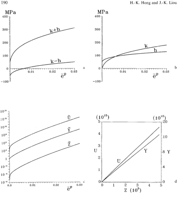
UFig. 3. Conversion of material functions of the stress-space rate-equation representation to those of the strain-controlled integral-equation representation a k(~ p) + h(~ p) determined from a uniaxial stress or tube-twisting test and k(~ p) - h(g p) determined from a series of reversed yielding tests b yield-stress function
h(~ p) and back-stress function k(0 p) in the stress-space plasticity e material functions 2,(~P), Y(0P), [7(gP) defined for use in converting h(~ p) and k(g v) to Y(Z) and U(Z) tl material functions Y(Z) and U(Z) for the strain-controlled integral-equation representation
Fig. 3 a, which then yield h(g;) and k(g;), as in Fig. 3 b. Next, plugging in the value of G, the functions Y(gP), 2(E v) and [7(E p) are respectively calculated out by Eqs. (19), (25) and (31), as in Fig. 3 c. Finally, from Eqs. (33) and (34), Y(Z) and U(Z) are determined, as in Fig. 3 d.
F r o m Eqs. (21)-(26) and (33)
ri/t)
Z(t) - Y(Z(t)) ru(t ) ~u(t ) = Y(Z(t)) 2G- eu(t)" (42)
2G
Since ru~ u is the power done by the active stress r~j, it m a y be justified to call it the active power and 2 the normalized active power and Z the normalized active work, in view of Eq. (42) and that
Integral-equation representations of flow elastoplasticity 191 J~(t) at the m o m e n t of the first-time yield from the zero-value time on is the active power at that time normalized in such a way it becomes the rate of the second invariant/2 of the deviatoric strain tensor e u, that is Z = [2 = d(eueu/2)/dt at that particular moment. Just as from Eq. (6) the effective plastic strain rate e p > 0 at any time, it can be shown from Eqs. (26), (41) and (6) that the normalized active power
2 >= 0 (43)
at any time. Hence, both the effective plastic strain
eP(t)
and the normalized active work Z(t) are monotonically increasing and dimensionless. The former m a y be deemed as a measure of intrinsic time for the stress-space rate-equation representation, whereas the latter a measure of intrinsic time for the strain-controlled integral-equation representation. Moreover, just as e p > 0 in a straining process,2 > 0 (44)
in a straining process.
Indeed, 2 > 0 is the straining condition for the strain-controlled integral-equation represen- tation. Whenever Z > 0 ceases to be valid, say, at time t,, Eq. (35) gives its way to
su(t) = sij(t.) + 2G[eij(t) - eu(tu)], (45)
where t. < t m a y be called the latest unloading time. Equation (45) governs until the yield condition for the integral-equation representation:
f 7(t.) if it has ever yielded
z(t)
(46)ay if it has never yielded
is impending to be satisfied, when Eq. (45) is replaced by Eq. (35). The ay = h(0) is the (initial) yield stress, or yield strength. To check Eq. (46), Eq. (8) and
rij(t) = re(t,) + sij(t) - sij(tu) (47)
have to be utilized.
In summary, the constitutive algebraic equation (45) and the constitutive integral equations (35)-(37), the straining condition, Eq. (44), and the yield condition, Eq. (46), constitute the deviatoric part of the strain-controlled integral-equation representation of the flow clastoplas- ticity.
5 Integration of rate equations given a stress history
When a stress history is given and the yield and straining conditions are satisfied, the constitutive rate equations can also be integrated to result in another integral-equation constitutive representation. Substitution of Eqs. (7), (4) and (5) into the identity (15) yields
kt~p
192 H.-K. Hong and J.-K. Liou which is an ordinary differential equation for the active stress and the solution of which can be readily written as
1[
;
1
rij(t) - y(~P(z)) rij(z) + Y(gP(~)) gij(~) d~ (49)
;(~p(t))
z where[i ]
k'(p)
y(~P) -- exp ~ dp (50) is a material function. Again from Eq. (48),k'~p
1;ijFij @ ~ rijrij = sijrij (51)
or, upon considering Eqs. (22) and (49),
(h' + k') he p = - - ;(Or(r)) ru(r ) + y(YP(r gu(~) cl~ . (52)
Y
Define
~p
~(~P) - ~ [h'(p) + U(p)] h(p) y(p) dp, e' = -3 (h' + k') hY, (53) 0
2
z(t) = z~(YP(t)), ~(t) = ~(eP(t)) = i ' e p = ~ (h' + k') hye p. (54)
Note that Z(~ p) is a material function while z(t) and ~P(t) are merely functions of time. From Eqs. (52) and (54),
or, after interchanging the order of integrations,
z(t) = z(r) + y(gP(z)) [su(t) - Su(Z)] ru(z) + i )7(gP(~)) [su(t ) - su(~) ] iu(~) d~. (56)
Next, combination of Eqs. (14), (29) and (49) yields
1 3eP(~)
~,(t) = Y d s,(t)
+ ~(~) +
2h(e~(~
~(e~(~)) ~(~(~))
~'j(~) +
Y(~Pr ~,j(O d~ d~.
(57)
Integral-equation representations of flow elastoplasticity 193 Define
g(6P) - 3Gy(6P) h(p) ~)(p)'
0
(58)
which is a material function. Interchanging the order of integrations in Eq. (57) and using definition (58) and once again Eqs. (14) and (49), we have
(59)
Having these expressions for ris(t), z(t) and eis(t), we m a y propose the following stress-controlled integral-equation representation.
6 Stress-controlled integral-equation representation
L e t y ( z ) -- ; ( i - l ( z ) ) = y(YP), u(z) - a ( e ~(~)) = a(~p). (6O)
(61)
F r o m Eqs. (51)-(54) and (60), rlj(t) .~(t) = y(z(t)) ro(t ) sij(t) = 2Gy(z(t)) 2 G - sis(t)" (62)
Since Rijgij(= rls~ij2G) is the c o m p l e m e n t a r y power due to the active strain R i j (which will be introduced later on and shown equal to rU2G ), it m a y be justified to call it the active c o m p l e m e n t a r y - p o w e r and ~ the normalized active complementary-power and z the normalized active complementary-work, in view of Eq. (62) and that 2(t) at the m o m e n t of the first-time yield from the zero-value time on is the active c o m p l e m e n t a r y - p o w e r at that m o m e n t normalized in such a way it becomes the rate of the second invariant Jz of the deviatoric stress tensor sij, that is
= J2 = d(sis&J2)/dt at that particular moment.
F r o m Eqs. (59)-(61), (56) and (49), the deviatoric strain e~s(t ) is given by
;,1
1
63,
eij(t) = eifir) + 2G
in which the normalized active c o m p l e m e n t a r y - w o r k z and the active stress ris are respectively calculated by
z(t) = z(z) + y(z(z)) [so(t ) -- sis(r)] ris(r) + i y(z(~)) Isis(t) -- sis(~)] sq(~) d~, (64)
r~s(t ) - y(z(r)) rij(~) + y(z(~)) sij(~) d~ . (65)
y(z(t))
194 H.-K. Hong and J.-K. Liou Since it is stress-controlled, the representation cannot apply to softening-plastic materials due to the material indeterminacy and is therefore restricted to hardening plasticity, for which
2
2 = y~uru = ~ yh(h' + k') e p > 0 (66)
in a straining process. Accordingly, Eq. (66), derived from Eqs. (62) and (13), is the straining condition for the stress-controlled integral-equation representation. Given deviatoric material properties G, ay = h(0), y(z) and u(z) and a time history of deviatoric stress, s u, the deviatoric strain is determined either by Eq. (63) with the aid of Eqs. (64) and (65) or by
1
eu(t ) = eu(t.) + ~ [su(t) - su(t~) ]. (67)
Whenever the straining condition for the integral-equation representation, Eq. (66), ceases to be valid, Eq.(63) gives its way to Eq. (67), which then governs until the yield condition, Eq. (46), is impending to be satisfied, at which time Eq. (67) is replaced by Eq. (63).
In summary, the constitutive algebraic equation (67), the constitutive integral equations (63)-(65), the straining condition (66), and the yield condition (46) constitute the deviatoric part of the stress-controlled integral-equation representation for hardening plasticity.
7 Strain-space rate-equation representation
Corresponding to the aforementioned stress-space rate-equation representation, the model problem can also be represented in strain space by specifying the yield function
F = / ] - H(~ r) < 0 (68)
on strain space and postulating that stress is relaxed from the elastic stress state by an a m o u n t called the stress relaxation:
= e _ ~ (69)
tYij tTij ~Tij,
in which the elastic part is governed by
si~ = 2Geij, a~k = 3~'su, (70)
and the relaxation part is governed by the evolution rules for the back strain A u and the stress relaxation si~- respectively, i.e.
3
AU = ~ K'(U) &5, Akk = 0, (71)
~F 2
&~i = s~ - - = sr - - R u , alk = 0, (72)
&u
3Hin which s r is implicitly defined and further required to confirm to s r ~ > 0 if /~ = H and RijO, lj > 0
(73)
(
= 0 otherwise,Integral-equation representations of flow elastoplasticity 195 where/~ = H, i.e. F = 0 is the yield condition in strain space and RijO~j > 0, i.e. F = 0 is the straining condition for the strain-space rate-equation representation. The superscripts e and r denote respectively the elastic and relaxation parts, and
Rij = eli - Aij (74)
is the active strain and
is the effective active-strain, always < H(g~). From Eqs. (72) and (73),
s-e = ( 2 SijSij) 1/2 , (76)
and the effective stress relaxation gr is
U = i st(z) dz, (77)
to
that is 3 ~ times the arc length of the path travelling in the stress relaxation space. At and before the zero-value time to, the material is in the zero-value (or virgin or free) state in which all relevant values vanish.
Constants and functions of material properties employed include the bulk modulus 2/{' (or Poisson's ratio v or Young's modulus E), shear modulus G, yield-strain function of material H(g r) and back-strain function of material K(gr).
Between the stress-space and strain-space representations there exist the following general relations. From Eqs. (2), (3), (5), (69), (70) and (72),
sit = 2Ge~, a~k = 3~{'e,~t = O. (78)
From these and Eqs.
(9), (10), (76) and (77),
s r = 3Ge p, gr = 3Gg p. (79)
In simultaneous and corresponding interpretations of test data collected from either the series of uniaxial stress tests or the series of tube-twisting tests, it can be shown, in view of the general relations, Eqs. (78) and (79), that the material functions of the stress-space and strain-space representations have the general relations:
H(g r ) = ~ h ~ , (80) /~(gr) = 3G k 3 d + 3T' (8~) and also h(g p) = 3GH(3G~P), k(e p) = 3GK(3Ge p) - 3GgP. (82)
(83)
196 H.-K. Hong and J.-K. Liou Besides these six Eqs. (78) trough (83), more equations can be established basing on these six equations and the relevant definitions and relations as follows:
slj = 2Ge~j, s~j = 2Geij, (84)
1
~ij = 2G(Aij - e~), Aij = ~ (~ij + siS), (85)
f = 3 G F , (86)
rij = 2GR~j, (87)
= 3 G ~ . (ss)
See Figs. 1 and 2.
In Eq. (73) the straining condition is written as
Rij~ij > 0, (89)
o r
P = 0, (90)
the necessary and sufficient condition of which is 3
Rij~ij = ~ H ( H ' + K') s r > 0, (91)
since combination of Eqs. (40), (82) and (83) yields
H ' + K' > 0. (92)
Equation (91) indeed covers, extensively, all hardening, perfect and softening plasticity. Therefore, in the strain-space representation, the positiveness of R~jOij always means straining for permissible ~ no matter whether the plasticity is hardening, perfect or softening. This favorite criterion motivated many researchers to appreciate the strain-space representation [6]-[8].
8 Integrations for strain-space model
Instead of starting with the stress-space rate-equation representation, we may start with the strain-space rate-equation representation just outlined in the preceding Section, following similar procedures and resulting in two integral-equation representations, one for the strain-controlled case and the other for the stress-controlled case. Skipping all details, we record final results as follows.
In the strain-controlled integral-equation representation, the deviatoric stress s~j is deter- mined by the constitutive algebraic equation
Integral-equation representations of flow elastoplasticity 197 or by the constitutive integral equation
sij(t) = su(z) + 2G { - U ( Z ( t ) ) Ru(O + U(Z(z)) Rij(z) + i [l + U(Z(())] ~ij(~) (94) in which the normalized active work Z and the active strain R u are calculated by the constitutive integral equations
Z(t) = Z(r) + Y(Z(z)) [eu(t ) - eu(z)] Ru(z ) + i Y(Z(~)) [e~j(t) - eu({) ] ~zj(~) d~, (95)
Y(Z(O) + e,j(r .
(96)
r
The yield condition is
/~(t) = {/~(t~) if it has ever yielded, (97)
~y if it has never yielded, and the straining condition is
2 > 0. (98)
To check Eq. (97), equations (75) and
1
Rij(t) = Rij(t.) + ~ [su(t) - su(t.)] (99)
have to be utilized.
In the stress-controlled integral-equation representation, the deviatoric strain e u is deter- mined by the constitutive algebraic equation (67) or by the constitutive integral equation
eij(t ) = eij(z) + ~ u(z(t)) 2GRij(t) - u(z(z)) 2GR,j(z) + [1 -- u(z(t))] sij(C) dC . (100)
in which the normalized active complementary-work z and the active strain Rij are calculated by the constitutive integral equations
z(t) = z(,) + y(z(z)) [su(t ) - su(,)] 2GRu(T ) + i y(z(~)) [su(t) - su(~)] gu(~) d~, (101)
z
Ru(t ) - y(z(z)) Ru(z ) + y(z(~)) su(~) d~ " (102)
-r
The yield condition is Eq. (97) and the straining condition is Eq. (66). This representation is not applicable to softening plasticity.
Comparison of these two representations obtained in this Section with those obtained from the stress-space model reveals that they are essentially identical, in view of Eq. (87). It is accordingly concluded that the integral-equation representations hardly distinguish which one,
198 H.-K. Hong and J.-K. Liou stress-space or strain-space, they are derived from, and that they have, however, very distinct forms depending on if the strain or the stress controls. This is quite different form the situation in the rate-equation representations. As a strain-controlled integral-equation representation, Eqs. (93)-(99) in this Section using the notions of strain space, mainly Rij replacing rij, are a little bit more precise than the corresponding ones using the notations of stress space. Although the two are almost identical, the more precise formulation in this Section is preferable and recommended. On the other hand, as a stress-controlled integral-equation representation, Eqs. (66), (67), (97) and (100)-(102) using the notations of strain space are a little bit less precise than the previous ones, Eqs. (46) and (63)-(67), which use the notions of stress space, mainly r u instead of R~j. The more precise equations, Eqs. (46) and (63)-(67), are recommended.
9 Calculation
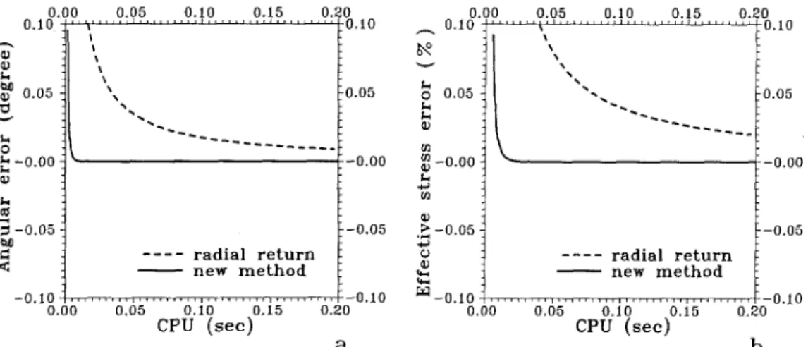
One of the immediate benefits derivable from the new representations is their adaptability for direct calculations; no sophisticated algorithms are needed except for simply and straightforwardly integrating the integrals. The calculations are completely tractable to any desired degree of precision. To have an idea of the convergence, efficiency and accuracy of the developed strain-controlled integral-equation representation, the C P U time con- sumption versus errors are plotted and compared with those obtained by using the widely used elastic predictor-radial return algorithm [9] of the classical stress-space rate-equation representation. Fig. 4 displays the results. Since the deviatoric stress sq can be effectively displayed on the ~-plane of the principal-deviatoric stress space (s~,s2,s3) where
s3 = - s l - s2 on which the yield condition becomes a circle with radius 2 ~ h(~P),
the accuracy of the output s~j can be completely revealed by the n o r m and angular errors on the z~-plane, which are both shown on the figures. It is found that both the new method and the radial return algorithm converge to the same digits and that the new method requires much less C P U time on a C O N V E X C1 computer for all cases investigated. F o r definiteness, Table 1 tabulates partial digital data, comparing, at the same degrees of precision, the C P U time consumption of the two methods. It is noted
0 . 0 0 0 . 0 5 O.lO 0 . 1 5 0 . 2 0 0 . 0 0 0.10 . . . . ~ . . . 0.10 0 . I 0 " %" 0 . 0 5 O - 0 . 0 0 ~9 - 0 . 0 5 < - 0 . 1 0 0 . 0 0 t \ . . . . r a d i a l r e t u r n n e w m e t h o d 0 . 0 5 - 0 . 0 0 - 0 . 0 5 0 . 0 5 0 . 1 0 0 . 1 5 0 . 2 0 . . . ~ . . . 0.10 v 0 . 0 5 -0.00 2 f/l .~ - 0 . 0 5 .t.J c) . . . . r a d i a l r e t u r n ~ n e w m e t h o d r"r-I - O. l 0 . . . , . . . 0.05 - 0 . 0 0 - 0 . 0 5 . . . - 0 . 1 0 - 0 . i 0 0 . 0 5 0 . 1 0 0 . 1 5 0 . 2 0 0 . 0 0 0 . 0 5 0 . 1 0 0 . 1 5 0 . 2 0 C P U ( s e c ) C P U ( s e e ) a b
Fig. 4. Convergence and accuracy versus efficiency compared between the new method and the radial return method a angular error b norm error of s u
Integral-equation representations of flow elastoplasticity 199 that, in a numerical simulation problem, the subroutine of the constitutive-equation solver m a y be called t h o u s a n d s of times; the errors thus induced are persistently a c c u m u l a t e d a n d p r o p a g a t e d . Therefore, to ensure an acceptably accurate, final result after the t h o u s a n d s of calls, the errors of each call must be k e p t definitively small, say, less t h a n 0.001% of the radius error and 0.001 ~ of the a n g u l a r error. F o r these levels of precision, the new m e t h o d is found to save 99 % or m o r e of the C P U time, as revealed in Table 1. The relevant properties of the m i x e d - h a r d e n i n g elastoplastic m a t e r i a l used for these investigations are G = 27040 M P a , ~y = h(0) = 52.66 M P a and Y(Z) a n d U(Z) shown in Fig. 3 d.
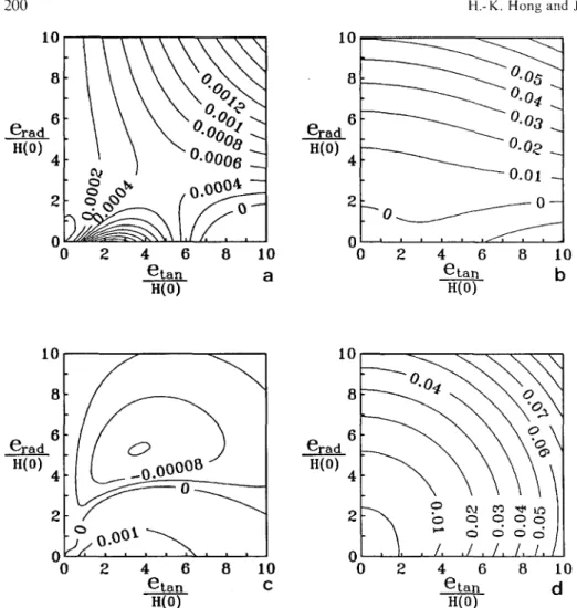
H a v i n g investigated convergence and the relation between efficiency and accuracy and d e m o n s t r a t e d the relative efficiency, we next perform error analyses by i n p u t t i n g a total of 900 different strain histories a n d studying the errors of the resulting outputs. T h e y are all linear paths with the same starting strain p o i n t (el, e2, es) = H(0) (0, 1, - 1) V ~ / 2 rigth on the initial relaxation circle b u t with 900 different ending strain points (%n, eraa). It is w o r t h noting that, since the r e l a x a t i o n surface of the considered m o d e l is a circle on the ~z-plane, whichever starting p o i n t on the initial relaxation circle is always a typical one and hence its circumferential position is irrelevant to the error analysis. Thus, the errors of the o u t p u t stresses for these input strain histories can be represented by a function of the tangential strain increment eta n a n d the r a d i a l strain increment eraa p r o v i d e d that the p a r t i c u l a r pattern, linear, q u a d r a t i c or others, of the input strain p a t h s is declared. This k i n d of study is therefore considered to be comprehensive and ever e m p l o y e d by m a n y authors, e.g. Krieg and Krieg [1], Schreyer et al. [10] and L o r e t and Prevost [111.
The results are shown in the form of percent isoerror contours on Fig. 5, in which a) for the a n g u l a r error of the deviatoric stress sij a n d b) for the error of the effective stress Y = (3sijs~/2) 1/2,
while c) for the a n g u l a r error of the active stress r o. a n d d) for the error of the effective active-stress ~ = (3r~ir~/2) 1/2, which are all o b t a i n e d by the new m e t h o d using 30 integration points, a m o u n t i n g to a b o u t 0.009 secs. C P U time as can be seen in Fig. 4. It is seen that the new m e t h o d seems quite favorable to h a r d l y have preferred strain p a t h directions. It c a n n o t be overemphasi- Table 1. CPU time consumed for different error levels. R.R. the radial return method; New new method;
R.R.-New
T.S. percentage of time saving - - - , * did not produce such a large error; ** was not able to reach
such accuracy R.R.
Angular CPU time
error
active stress rij deviatoric stress Sij
(degree) R.R. New T.S. R.R. New TS. 1 ~ 0.0147 * - * * - 0.1 ~ 0.1215 0.0017 98.6% 0.016 3 0.0017 89.6% 0.01 ~ 1.2069 0.0038 99.7% 0.1744 0.0038 97.8% 0.001 ~ 10.8919 0.0081 99.9% 1.7622 0.0081 99.5%
Norm CPU time
error
active stress r U deviatoric stress sij
R.R. New T.S. R.R. New T.S.
0.1% 0.0221 0.0051 76.9% 0.039 5 0.005 2 86.8%
0.01% 0.1804 0.0119 93.4% 0.389 4 0.0110 97.2%
0.001% ** 0.030 5 > 99.9% 2.487 9 0.0201 99.2%
200 10 6 e r a d
a(o)
4 I0 8 (3 erad n(o) 4)
ooa Z
0 ' 0 0 2 4 6 8 10 0 e t a n a H(O)H.-K. Hong and J.-K. Liou
~ " 0 . 0 ~ ~ 0 . 0 1 -_. 0 ~ _ / 0 -- I I I I I I ~ 2 4 6 8 10 e t a n b 0 8 8 - 0 04
e
e
H(O)
H(0)
2 / 2 b a 0 ~ ' d ," , . . , " . , 0 ' '/' ' / ' /' /' /'
0 2 4 6 8 10 0 2 4 6 8 tO e t a n c e t a n dn(o)
H(O)
Fig. 5. Percent isoerror maps for the method, which is favorable to hardly have preferred directions of strain paths a angular error of the deviatoric stress s u b norm error ofs o c angular error of the active stress rq d norm error of rij
zed that, since the new integral-equation representations can e m b o d y any input path (without such an assumption of constant strain rate or linear strain path, for example), the more complex the input strain path is, the more advantageous the present method is.
10 Relaxation and creep functions
It is interesting to explore that Eqs. (35)-(37) or (94)-(96) of the strain-controlled integral- equation representation can be put into the following viscoelasticity-like form:
i G(Z(t), Z(~)) ~A~) d~, (103)
- c o
s~j(t) =
where
Integral-equation representations of flow elastoplasticity 201 is the normalized active work and
G(Z1,
Z2) ~ 2G I1 + g ( z 2 ) -- g ( Z l )Y(Z2)~y(z1)j
(105)is a material function called the shear relaxation function of elastoplasticity, Z1 and Z2 being the output and input normalized active works, respectively.
Similarly, Eqs. (63)-(65) or (100)-(102) of the stress-controlled integral-equation represen- tation can be arranged to be
e,j(t) = i J(z(t), z(~)) gij(~) d~,
(106)where
z(t) = j! y(z(~)) [sij(t) - s~j(~)] ~ij(~) d~
(107)
-co
is the normalized active complementary-work and
1 [
y(z2)~
(108)
J ( z l , z2) - 2 d 1 - u(z2) + u(z~)
Y(z~)J
is a material function called the shear creep function of elastoplasticity, z~ and z2 being the output and input normalized active complementary-works, respectively.
The lower limits of integrations of the integrals in Eqs. (103), (104), (106) and (107) can be replaced by to.
11 Concluding remarks
We have composed the separately specified ingredients of the rate-equation representations of the flow elastoplasticity and exactly integrated the rate equations to integral equations. The natural definitions of the material functions in terms of the normalized active work or complementary-work enable us to establish the two integral-equation representations. The two rate-equation and two integral-equation representations represent four distinct but intimate point-of-views on the same material behavior. Each of the four representations is self-contained and can be independently manipulated.
In the rate-equation representations, the plastic mechanism is described mainly in terms of the evolution of internal state variables, whereas in the integral-equation representations the highly nonlinear path-dependence is so unfolded that a detour to the evolution of internal state variables is obsolete. For each of the four representations, there exists a measure of intrinsic time, the effective plastic strain YP for the stress-space rate-equation representation, the effective stress relaxation U for the strain-space rate-equation representation, the normalized active work Z for the strain-controlled integral-equation representation, and the normalized active complemen- tary-work z for the stress-controlled integral-equation representation.
Someone may tend to deem, in view of similarity of appearances, the strain-controlled integral-equation representation developed herein to be a new version of the endochronic theory, as a constructive reinforcement and reform to the first and second versions of the theory [12] - [14]. However, it is observed that the intrinsic time of each of the four representations is not only related to the property of material but also depends explicitly on the history of input.
202 H.-K. Hong and J.-K. Liou: Integral-equation representations of flow elastoplasticity The strain-controlled integral-equation r e p r e s e n t a t i o n is well tested and the extensive verifications d e m o n s t r a t e that the calculations based on it are much m o r e accurate and faster t h a n the widely used r a d i a l return a l g o r i t h m of the r a t e - e q u a t i o n representations. Time saving is r e m a r k a b l y high, say, 99% or m o r e at a realistic level of accuracy; moreover, the errors are controllable and assessable. O n the other hand, a possible d e v e l o p m e n t of constitutive laws directly from integral kernels a n d / o r functional representation seems to have opened a way of thinking and experimentation.
References
[1] Krieg, R. D., Krieg, D. B.: Accuracies of numerical solution methods for the elastic-perfectly plastic model. J. Press. Vess. Tech. 99, 510-515 (1977).
[2] Nagtegaal, J. C., Parks, D. M., Rice J. R. : On numerically accurate finite element solutions in the fully plastic range. Comput. Meth. Appl. Mech. Eng. 4, 153-177 (1974).
[3] Ortiz, M., Popov, E. R: Accuracy and stability of integration algorithms for elastoplastic constitutive relations. Int. J. Num. Meths. Eng. 21, 1561-1567 (1985).
[4] Hong, H.-K., Lan. H.-S.: A new point-of-view at plastic materials of the Prandtl-Reuss type. In: Advances in plasticity 1989 (Khan, A. S., Tokuda, M., eds), pp. 95-98, 1989.
[5] Drucker, D. C.: Conventional and nonconventional plastic response and representation. Appl. Mech. Rev. 41, 151-167 (1988).
[6] Naghdi, R M., Trapp, J. A.: The significance of formulating plasticity theory with reference to loading surfaces in strain space. Int. J. Eng. Sci. 13, 785-797 (1975).
[7] Lubliner, J.: A simple theory of plasticity. Int. J. Sol. Struct. 10, 313-319 (1974).
[8] Yoder, R J., McDowell, D. L, : Bounding-surface plasticity: stress space versus strain space. Acta Mech. 77, 1 3 - 4 5 (1989).
[9] Simo, J. C., Taylor, R, L.: Consistent tangent operators for rate-independent elastoplasticity. Comput. Meth. Appl. Mech. Engng. 48, 101-118 (1985).
[10] Schreyer, H. L., Kulak, R. E, Kramer, J. M.: Accurate numerical solutions elastic-plastic model. J. Press. Vess. Tech. 101, 226-234 (1979).
[11] Loret, B., Prevost, J. H.: Accurate numerical solutions for Drucker-Prager elastic-plastic models. Comput. Meth. Appl. Mech. Eng. 54, 259--277 (1986).
[12] Valanis, K. C.: On the foundations of the endochronic theory of viscoplasticity. Arch. Mech. 27, 857-868 (1975).
[13] Valanis, K. C.: Fundamental consequences of a new intrinsic time measure plasticity as a limit of the endochronic theory. Arch. Mech. 32, 171-191 (1980).
[14] Wu, H. C., Yeh, M. C.: Some considerations in the endochronic description of anisotropic hardening. Acta Mech. 69, 5 9 - 7 6 (1987).
Authors' addresses: Prof. Dr. H.-K. Hong, Department of Civil Engineering, National Taiwan University, Taipei 10764, and Dr. J.-K. Liou, Associate Research Scientist, Chung-Shan Institute of Science and Technology, P.O. Box 90008-15-9, Lungtan, Taoyuan 32526, Taiwan, Republic of China